On the Diversity Constraints for Portfolio Optimization

Abstract

In the literature, Markowitz’s mean-variance model and its variants have been shown to yield portfolios that put excessive weights on only a few assets. Many diversity constraints were proposed and added to these models to avoid such overly concentrated portfolios. However, since these diversity constraints are formulated differently, it becomes difficult to compare them and study their relationships. This paper proposes a canonical form for the commonly used diversity constraints in the literature, and shows how to transform these diversity constraints into this canonical form. Furthermore, this paper compares these diversity constraints (in the canonical form with the same upper bound) on their ability to shrink the feasible region of the portfolio optimization problem. The results show a subset relation among their feasible regions.

1. Introduction

Portfolio optimization deals with the problem of allocating one’s wealth across a number of assets to maximize return and control risk. This problem was first studied in the seminal paper of Markowitz [1], who proposed a mathematical formulation of the problem, and derived a mean-variance model to yield portfolios that either maximize the portfolio expected return for a given level of risk, or minimize the portfolio risk for a given expected return. Since then, this problem continues to receive much consideration and attention from both academics and practitioners in the financial industry, and many variants of the mean-variance model (e.g., minimum-variance model, mean-variance-skewness model, etc.) have been proposed. Please refer to [2,3,4] for the variants of the mean-variance model.

Markowitz’s mean-variance model uses the expected return of each asset and the covariance between the returns of any two assets as input. In practice, these input values are hard to estimate with high accuracy, and the estimations based on historical data might not be appropriate for future data. Furthermore, the portfolios derived from the mean-variance model are very sensitive to these input values [5,6]. Consequently, mean-variance optimized portfolios often put excessive weights on assets with large expected returns [6,7], regardless of possible estimation errors in these input values. Such overly concentrated portfolios, which also occur in the variants of the mean-variance model [3], go against the idea of diversification. DeMiguel et al. compared several variants of the mean-variance model on several datasets, and showed that none of these models consistently beat the naïve equally-weighted portfolio, out of sample [4].

To reduce the impact of estimation error and avoid overly concentrated portfolios, several diversity constraints have been introduced in the literature. The weight upper/lower bound constraint [8] simply imposes an upper/lower bound on assets’ weights in a portfolio. The L^p-norm constraint [9] and the entropy constraint [10] impose an upper bound on the L^p-norm and a lower bound on the entropy, of the assets’ weights in a portfolio, respectively. Empirical studies [8,9,11] show the weight upper bound constraint or the L^p-norm constraint improves portfolio efficiency out of sample. Using the entropy of the assets’ weights as one of the objective functions in a multi-objective setting also improves portfolio efficiency out of sample [2].

Even though these diversity constraints improve the out-of-sample performance of the portfolio optimization problem, their relation remains unclear. To the best of our knowledge, no work compares these diversity constraints on their abilities to shrink the feasible region of the portfolio optimization problem. One reason hindering such a comparison is due to the differences among these diversity constraints. Notably, some diversity constraints are in the form of an upper bound, but others are in the form of a lower bound. Furthermore, the ranges of their respective bounds are also different. Consequently, it is difficult to compare them systematically.

The objective of this study is to provide a systematic way to compare the performance of these diversity constraints. To achieve this goal, we first propose a canonical form for these diversity constraints, and show how to transform these diversity constraints into the canonical form. With the canonical form, all of these diversity constraints are in the form of an upper-bound constraint, and their respective bounds all fall into the same range. On the lowest end of the range of the bounds, these diversity constraints all restrict the feasible region of the portfolio optimization problem to exactly one point corresponding to the equally-weighted portfolio. On the highest end of the range of the bounds, these diversity constraints all become redundant. By using the same value for the upper bound of these diversity constraints in the canonical form, a systematical comparison among them can be achieved. Although these diversity constraints diminish the feasible region of the portfolio optimization problem differently, a subset relation among their feasible regions can be derived for these diversity constraints in the canonical form under the same upper-bound value.

The rest of this paper is organized as follows: Section 2 reviews the commonly used diversity constraints in the literature, including the weight upper/lower bound constraint, the L^p-norm constraint and the entropy constraint. Section 3 proposes the canonical form for these diversity constraints and shows how to transform them into the canonical form. Section 4 discusses the subset relation among these diversity constraints. Section 5 studies how the feasible region of the portfolio optimization problem shrinks as these diversity constraints are applied. Section 6 concludes this paper.

2. Review of Diversity Constraints

Diversifying a portfolio avoids putting too much weight on only a few assets. This has the potential of reducing risk of the portfolio. Adding an upper-bound constraint on assets’ weights is probably the most common and simplest way to control the diversity of a portfolio. In practice, institutional investors are often restricted by law to enforce such a weight upper-bound constraint [12]. Diversifying a portfolio can also be achieved by imposing a lower-bound constraint on assets’ weights or by restricting the L^p-norm or the entropy of the assets’ weights of a portfolio. This section reviews these commonly used diversity constraints in the literature.

For ease of exposition, this study considers the following base form of the portfolio optimization problem where short selling is prohibited.

Problem 1. Given the expected returns of n risky assets $\mathbf{r}=(r_1,r_2,\dots ,r_n)$ and their variance-covariance matrix $\mathsf{\sigma }={({\sigma }_{ij})}_{n\times n}$, find a portfolio $\mathbf{w}=(w_1,w_2,\dots ,w_n)$ such that the objective function $f(\mathbf{w})$ is maximized, subject to the following two constraints:

$$0\le w_i\le 1, \mathrm{for} i=1 \mathrm{to} n$$

(1)

$${\sum }_{i=1}^n{w}_i=1$$

(2)

The constraint in Equation (1) prohibits short selling by restricting to non-negative weights. Notably, a non-negative weight is required for calculating the entropy of $\mathbf{w}$, to be defined shortly in Section 2.4. The constraint in Equation (2) enforces that all wealth is invested. The objective function $f(\mathbf{w})$ often involves maximizing the portfolio’s return and/or minimizing the portfolio’s risk. For example, Markowitz’s mean-variance model uses $\mathbf{r}{\mathbf{w}}^T$ and $\mathbf{w}\mathsf{\sigma }{\mathbf{w}}^T$ to measure the expected return and the risk of a portfolio $\mathbf{w}$, respectively [1], and therefore, $f(\mathbf{w})$ can be defined as $\frac{\mathbf{r}{\mathbf{w}}^T}{\mathbf{w}\mathsf{\sigma }{\mathbf{w}}^T}$ or $\mathbf{r}{\mathbf{w}}^T-\mathbf{w}\mathsf{\sigma }{\mathbf{w}}^T$ for finding a comprise between return and risk.

2.1. Weight Upper-Bound Constraint

The weight upper-bound constraint directly avoids the overly concentrated portfolios by adding an upper bound ${\mathrm{U}}_{\mathrm{W}}$ on the weight of each asset in a portfolio. It is expressed as follows:

$$\max (\mathbf{w})\le {\mathrm{U}}_{\mathrm{W}}$$

(3)

Notably, $\max (\mathbf{w})$ returns the maximum component of $\mathbf{w}$. With the weight upper-bound constraint, smaller ${\mathrm{U}}_{\mathrm{W}}$ restricts the feasible region of Problem 1 only to the more diverse portfolios. On one extreme, if ${\mathrm{U}}_{\mathrm{W}}=\frac{1}{n}$, then the feasible region of Problem 1 contains only one portfolio, i.e., the equally-weighted portfolio. On the other extreme, if ${\mathrm{U}}_{\mathrm{W}}$ = 1, constraint in Equation (3) becomes redundant due to constraint in Equation (1). Therefore, the range of ${\mathrm{U}}_{\mathrm{W}}$ is $[\frac{1}{n},1]$.

2.2. Weight Lower-Bound Constraint

Imposing a lower bound on the assets’ weights can also avoid overly concentrated portfolios. The weight lower-bound constraint is expressed as follows:

$$\min (\mathbf{w})\ge {\mathrm{L}}_{\mathrm{W}}$$

(4)

Notably, $\min (\mathbf{w})$ returns the minimum component of $\mathbf{w}$. With the weight lower-bound constraint, larger ${\mathrm{L}}_{\mathrm{W}}$ restricts the feasible region of Problem 1 only to more diverse portfolios. On one extreme, if ${\mathrm{L}}_{\mathrm{W}}=\frac{1}{n}$, then the feasible region of Problem 1 contains only one portfolio, i.e., the equally-weighted portfolio. On the other extreme, if ${\mathrm{L}}_{\mathrm{W}}=0$, constraint in Equation (4) becomes redundant due to constraint in Equation (1). Therefore, the range of ${\mathrm{L}}_{\mathrm{W}}$ is $[0,\frac{1}{n}]$.

Lemma 1.

Consider Problem 1. Given ${\mathrm{L}}_{\mathrm{W}}\in [0,\frac{1}{n}]$, if $\min (\mathbf{w})\ge {\mathrm{L}}_{\mathrm{W}}$, then $\max (\mathbf{w})\le 1-(n-1){\mathrm{L}}_{\mathrm{W}}$.

Proof. 

Since $\min (\mathbf{w})\ge {\mathrm{L}}_{\mathrm{W}}$, the upper bound of the weights occurs when n-1 components of $\mathbf{w}$ all equal ${\mathrm{L}}_{\mathrm{W}}$ and the remaining component of $\mathbf{w}$ equals $1-(n-1){\mathrm{L}}_{\mathrm{W}}\ge {\mathrm{L}}_{\mathrm{W}}$. Thus, $\max (\mathbf{w})\le 1-(n-1){\mathrm{L}}_{\mathrm{W}}$. □

Lemma 1 shows that enforcing a weight lower-bound constraint also imposes a weight upper-bound constraint, which in turn avoids the overly concentrated portfolios. It can be used to check for redundant weight upper-bound constraint when both upper bound and lower bound on assets’ weights are applied. For example, consider Problem 1 subject to both constraints in Equations (3) and (4) with ${\mathrm{L}}_{\mathrm{W}}=0.01$, ${\mathrm{U}}_{\mathrm{W}}=0.91$ and $n=11$. By Lemma 1, $\min (\mathbf{w})\ge 0.01$ implies $\max (\mathbf{w})\le 0.9$, and thus $\max (\mathbf{w})\le 0.91$ is redundant.

2.3. L^p-norm Constraint

Given $p>1$, the L^p-norm constraint adds an upper bound ${\mathrm{U}}_{\mathrm{N}}$ on the L^p-norm $\mathrm{N}(\mathbf{w})$ of a portfolio $\mathbf{w}$, as defined below:

$$\mathrm{N}(\mathbf{w})={\sum }_{i=1}^n{\left|w_i\right|}^p\le {\mathrm{U}}_{\mathrm{N}}$$

(5)

In the least diverse scenario wherein only one component of $\mathbf{w}$ is 1 and the rest of the components of $\mathbf{w}$ are 0, $\mathrm{N}(\mathbf{w})$ reaches its maximum 1. In the most diverse scenario that $w_i=\frac{1}{n}$ for all i, $\mathrm{N}(\mathbf{w})$ reaches its minimum $n{(\frac{1}{n})}^p=n^{1-p}$. Therefore, the range of ${\mathrm{U}}_{\mathrm{N}}$ is $[n^{1-p},1]$. With the L^p-norm constraint, smaller ${\mathrm{U}}_{\mathrm{N}}$ restricts the feasible region of Problem 1 to more diverse portfolios.

Lemma 2 shows that enforcing an L^p-norm constraint also imposes a weight upper-bound constraint. Therefore, similar to Lemma 1, Lemma 2 can be used to check for redundant weight upper-bound constraint when both the weight upper-bound constraint and the L^p-norm constraint are applied.

Lemma 2.

Consider Problem 1. Given ${\mathrm{U}}_{\mathrm{N}}\in [n^{1-p},1]$ and $p>1$, if $\mathrm{N}(\mathbf{w})\le {\mathrm{U}}_{\mathrm{N}}$, then $\max (\mathbf{w})\le {({\mathrm{U}}_{\mathrm{N}})}^{\frac{1}{p}}$.

Proof. 

Prove by contradiction. Assume that $\mathbf{w}$ has a component $w_j>{({\mathrm{U}}_{\mathrm{N}})}^{\frac{1}{p}}$. Then, $p>1$ yields $w_j^p>{\mathrm{U}}_{\mathrm{N}}$. Since $w_i\ge 0$ for all i, ${\sum }_{i\ne j}{w}_i^p\ge 0$. Then, $\mathrm{N}(\mathbf{w})=w_j^p+{\sum }_{i\ne j}{w}_i^p>{\mathrm{U}}_{\mathrm{N}}$, which contradicts to $\mathrm{N}(\mathbf{w})\le {\mathrm{U}}_{\mathrm{N}}$ □

DeMiguel et al. proposed the A-norm constraint as $\mathbf{wA}{\mathbf{w}}^T\le \delta$, where $\mathbf{A}\in {ℝ}^{n\ast n}$ is a positive definite matrix [9]. Even though the A-norm constraint lets the investors incorporate their preference about the assets into the matrix $\mathbf{A}$, the matrix $\mathbf{A}$ can be hard to decide. Therefore, the identity matrix is often used for the matrix $\mathbf{A}$, and the A-norm becomes the L^p-norm with $p=2$.

2.4. Entropy Constraint

The entropy constraint adds a lower bound ${\mathrm{L}}_{\mathrm{E}}$ on the entropy $\mathrm{E}(\mathbf{w})$ of a portfolio $\mathbf{w}$, as defined below [10]:

$$\mathrm{E}(\mathbf{w})=-{\displaystyle \sum _{i=1}^n}{w}_i\ln w_i\ge {\mathrm{L}}_{\mathrm{E}}$$

(6)

In the least diverse scenario that only one component of w is 1 and the rest of the components of w are 0, $\mathrm{E}(\mathbf{w})$ reaches its minimum −1× ln1=0. In the most diverse scenario that $w_i=\frac{1}{n}$ for all i, $\mathrm{E}(\mathbf{w})$ reaches its maximum $-n(\frac{1}{n}\ln \frac{1}{n})=\ln n$. Thus, the range of ${\mathrm{L}}_{\mathrm{E}}$ is $[0,\ln n]$. Since a larger $\mathrm{E}(\mathbf{w})$ indicates better diversity, the entropy constraint uses a lower bound ${\mathrm{L}}_{\mathrm{E}}$ within the interval $[0,\ln n]$ to control the diversity of w from being too low.

Lemma 3.

Consider Problem 1. Given ${\mathrm{U}}_{\mathrm{W}}\in [\frac{1}{n},1]$, if $\max (\mathbf{w})\le {\mathrm{U}}_{\mathrm{W}}$, then $\mathrm{E}(\mathbf{w})\ge -\ln ({\mathrm{U}}_{\mathrm{W}})$.

Proof. 

The minimum of $\mathrm{E}(\mathbf{w})$ occurs at the least diverse portfolio. Since ${\mathrm{U}}_{\mathrm{W}}\in [\frac{1}{n},1]$, in the least diverse portfolio, $\lfloor \frac{1}{{\mathrm{U}}_{\mathrm{W}}}\rfloor$ assets each has the maximum weight ${\mathrm{U}}_{\mathrm{W}}$, one asset has the remaining weight 1 − $\lfloor \frac{1}{{\mathrm{U}}_{\mathrm{W}}}\rfloor {\mathrm{U}}_{\mathrm{W}}$, and the rest of the assets have weight zero. Then, $0\le 1-\lfloor \frac{1}{{\mathrm{U}}_{\mathrm{W}}}\rfloor {\mathrm{U}}_{\mathrm{W}}<{\mathrm{U}}_{\mathrm{W}}\le 1$ yields $\ln (1-\lfloor \frac{1}{{\mathrm{U}}_{\mathrm{W}}}\rfloor {\mathrm{U}}_{\mathrm{W}})<\ln {\mathrm{U}}_{\mathrm{W}}\le \ln (1)=0$. Consequently, the lower bound of $\mathrm{E}(\mathbf{w})$ can be derived as follows:

Lemma 3 shows that using a weight upper-bound constraint can impose an entropy constraint. Notably, the converse of Lemma 3 does not hold. That is, $\mathrm{E}(\mathbf{w})\ge -\ln ({\mathrm{U}}_{\mathrm{W}})$ for some ${\mathrm{U}}_{\mathrm{W}}\in [\frac{1}{n},1]$ does not imply $w_i\le {\mathrm{U}}_{\mathrm{W}}$ for all i. For example, if $\mathbf{w}=(\frac{1}{2}, \frac{1}{6}, \frac{1}{6}, \frac{1}{6})$ and ${\mathrm{U}}_{\mathrm{W}}=\frac{1}{3}$, then $\mathrm{E}(\mathbf{w})=\ln ({12}^{\frac{1}{2}})\ge -\ln ({\mathrm{U}}_{\mathrm{W}})$ but w₁ = $\frac{1}{2}\ge {\mathrm{U}}_{\mathrm{W}}$.

3. Canonical Form of Diversity Constraints

Tightening the bounds for the four diversity constraints described in Section 2 all shrink the feasible region of Problem 1 gradually to the equally-weighted portfolio. However, the four diversity constraints shrink the feasible region differently, and the relation among them remains unclear. Furthermore, determining the bound for the weight upper/lower bound constraint may be intuitive for the investors, but this is not the case for the L^p-norm constraint and the entropy constraint. To facilitate the comparison among the four diversity constraints, this section proposes the canonical form of a diversity constraint as follows:

$$D(\mathbf{w})\le U$$

(7)

where $D(\mathbf{w})$ is a scalar function of $\mathbf{w}$ for the diversity constraint, and the upper bound $U$ is confined to the interval $[\frac{1}{n},1]$.

In the canonical form, all of these diversity constraints are in the form of an upper-bound constraint, and the ranges of their respective bounds are all $[\frac{1}{n},1]$. Consequently, these diversity constraints can be compared under the same upper bound. Obviously, the weight upper-bound constraint is already in the canonical form by simply letting $D(\mathbf{w})=\max (\mathbf{w})$ and $U={\mathrm{U}}_{\mathrm{W}}$. The rest of this section shows how to transform the remaining three diversity constraints into this canonical form.

3.1. Transforming Weight Lower-Bound Constraint

The weight lower-bound constraint, defined in Equation (4), can be transformed into the following upper-bound constraint:

$$\mathrm{L}(\mathbf{w})=1+(1-n)\min (\mathbf{w})\le {\mathrm{U}}_{\mathrm{L}}$$

(8)

Lemma 4 shows that constraint in Equation (8) with ${\mathrm{U}}_{\mathrm{L}}=1+(1-n){\mathrm{L}}_{\mathrm{W}}$ is equivalent to the weight lower-bound constraint in Equation (4).

Lemma 4.

Consider Problem 1. Given ${\mathrm{L}}_{\mathrm{W}}\in [0,\frac{1}{n}]$, $\mathrm{L}(\mathbf{w})\le {\mathrm{U}}_{\mathrm{L}}=1+(1-n){\mathrm{L}}_{\mathrm{W}}$ iff $\min (\mathbf{w})\ge {\mathrm{L}}_{\mathrm{W}}$.

Proof. 

Since $1-n\le 0$, $\min (\mathbf{w})\ge {\mathrm{L}}_{\mathrm{W}}\ge 0$ iff $\mathrm{L}(\mathbf{w})=1+(1-n)\min (\mathbf{w})\le 1+(1-n){\mathrm{L}}_{\mathrm{W}}={\mathrm{U}}_{\mathrm{L}}$ .

Since the range for the lower bound ${\mathrm{L}}_{\mathrm{W}}$ in Equation (4) is $[0,\frac{1}{n}]$, the range for the upper bound ${\mathrm{U}}_{\mathrm{L}}$ in Equation (8) is $[\frac{1}{n},1]$. Transforming the weight lower-bound constraint in Equation (4) into the canonical form can be done by setting $D(\mathbf{w})=\mathrm{L}(\mathbf{w})$ and $U={\mathrm{U}}_{\mathrm{L}}=1+(1-n){\mathrm{L}}_{\mathrm{W}}$.

3.2. Transforming L^p-norm Constraint

The range for the upper bound ${\mathrm{U}}_{\mathrm{N}}$ in the L^p-norm Equation (5) is the interval $[n^{1-p},1]$, which varies with the value of p. The L^p-norm constraint can be transformed into Equation (9) such that the range of the upper bound becomes independent of the value of p:

$${\mathrm{N}}_p(\mathbf{w})={(\mathrm{N}(w))}^{\frac{1}{p-1}}={({\sum }_{i=1}^n{\left|w_i\right|}^p)}^{\frac{1}{p-1}}\le {\mathrm{U}}_{\mathrm{N}p}$$

(9)

Since the range of ${\mathrm{U}}_{\mathrm{N}}$ in Equation (5) is the interval $[n^{1-p},1]$ and ${\mathrm{N}}_p(\mathbf{w})$ is the (p−1)-root of $\mathrm{N}(\mathbf{w})$, the range of ${\mathrm{U}}_{\mathrm{N}p}$ in Equation (9) is $[\frac{1}{n},1]$. Furthermore, Equation (9) with ${\mathrm{U}}_{\mathrm{N}p}={({\mathrm{U}}_{\mathrm{N}})}^{\frac{1}{p-1}}$ is equivalent to Equation (5). Transforming the L^p-norm constraint in Equation (5) into the canonical form can be done by setting $D(\mathbf{w})={\mathrm{N}}_p(\mathbf{w})$ and $U={\mathrm{U}}_{\mathrm{N}p}={({\mathrm{U}}_{\mathrm{N}})}^{\frac{1}{p-1}}$.

Similar to Lemma 2, Lemma 5 shows that using constraint in Equation (9) also imposes a weight upper-bound constraint.

Lemma 5.

Consider Problem 1. Given ${\mathrm{U}}_{\mathrm{N}p}\in [\frac{1}{n}, 1]$ and $p>1$, if ${\mathrm{N}}_p(\mathbf{w})\le {\mathrm{U}}_{\mathrm{N}p}$, then $\max (\mathbf{w})\le {({\mathrm{U}}_{\mathrm{N}p})}^{\frac{p-1}{p}}$.

Proof. 

Proof by contradiction. Assume that $\mathbf{w}$ has a component $w_j>{({\mathrm{U}}_{\mathrm{N}p})}^{\frac{p-1}{p}}$. Then, $p>1$ yields $w_j^p>{({\mathrm{U}}_{\mathrm{N}p})}^{p-1}$. Since $w_i\ge 0$ for all i, ${\sum }_{i\ne j}{w}_i^p\ge 0$. Then, ${\mathrm{N}}_p(\mathbf{w})={(w_j^p+{\sum }_{i\ne j}{w}_i^p)}^{\frac{1}{p-1}}>{({{\mathrm{U}}_{\mathrm{N}p}}^{p-1})}^{\frac{1}{p-1}}={\mathrm{U}}_{\mathrm{N}p}$, which contradicts to ${\mathrm{N}}_p(\mathbf{w})\le {\mathrm{U}}_{\mathrm{N}p}$.

By Lemma 5, Equation (9) with ${\mathrm{U}}_{\mathrm{N}p}=1$ is redundant since it only restricts all weights to less than or equal to 1. Lemma 6 considers the case of ${\mathrm{U}}_{\mathrm{N}p}<1$.

Lemma 6.

Consider Problem 1. Given ${\mathrm{U}}_{\mathrm{N}p}\in [\frac{1}{n}, 1)$ and $p>1$, if ${\mathrm{N}}_p(\mathbf{w})\le {\mathrm{U}}_{\mathrm{N}p}$, then $\max (\mathbf{w})<{({\mathrm{U}}_{\mathrm{N}p})}^{\frac{p-1}{p}}$.

Proof. 

Proof by contradiction. Assume that $\mathbf{w}$ has a component $w_j\ge {({\mathrm{U}}_{\mathrm{N}p})}^{\frac{p-1}{p}}$. Then, $p>1$ and ${\mathrm{U}}_{\mathrm{N}p}\in [\frac{1}{n}, 1)$ yield $w_j^p\ge {({\mathrm{U}}_{\mathrm{N}p})}^{p-1}$ and ${({\mathrm{U}}_{\mathrm{N}p})}^{\frac{p-1}{p}}\ne 1$. Since $w_j\ge {({\mathrm{U}}_{\mathrm{N}p})}^{\frac{p-1}{p}}\ne 1$ and ${\sum }_{i=1}^n{w}_i=1$, there exists some $k\ne j$ such that $w_k>0$. Consequently, ${\sum }_{i\ne j}^{\square }{w}_i^p>0$. Then, ${\mathrm{N}}_p(\mathbf{w})={(w_j^p+{\sum }_{i\ne j}{w}_i^p)}^{\frac{1}{p-1}}>{\mathrm{U}}_{\mathrm{N}p}$, which contradicts to ${\mathrm{N}}_p(\mathbf{w})\le {\mathrm{U}}_{\mathrm{N}p}$.

Conversely, like Lemma 3, enforcing a weight upper-bound constraint can also impose an upper bound on the L^p-norm of $\mathbf{w}$, as shown in Lemma 7.

Lemma 7.

Consider Problem 1. Given ${\mathrm{U}}_{\mathrm{W}}\in [\frac{1}{n},1]$, if $\max (\mathbf{w})\le {\mathrm{U}}_{\mathrm{W}}$, then ${\mathrm{N}}_p(\mathbf{w})\le {\mathrm{U}}_{\mathrm{W}}$.

Proof. 

The proof is similar to that of Lemma 3. The maximum of ${\mathrm{N}}_p(\mathbf{w})$ occurs at the least diverse portfolio. Since ${\mathrm{U}}_{\mathrm{W}}\in [\frac{1}{n},1]$ and $\max (\mathbf{w})\le {\mathrm{U}}_{\mathrm{W}}$, in the least diverse portfolio, $\lfloor \frac{1}{{\mathrm{U}}_{\mathrm{W}}}\rfloor$ assets each has the maximum weight ${\mathrm{U}}_{\mathrm{W}}$, one asset has the remaining weight 1 − $\lfloor \frac{1}{{\mathrm{U}}_{\mathrm{W}}}\rfloor {\mathrm{U}}_{\mathrm{W}}$, and the rest of the assets have weight zero. Obviously, $0\le 1-\lfloor \frac{1}{{\mathrm{U}}_{\mathrm{W}}}\rfloor {\mathrm{U}}_{\mathrm{W}}<U_{\mathrm{W}}$. Finally, the upper bound of ${\mathrm{N}}_p(\mathbf{w})$ can be calculated as follows:

3.3. Transforming Entropy Constraint

The entropy constraint, defined in Equation (6), can be transformed into an upper-bound constraint as follows:

$$\mathrm{F}(\mathbf{w})=e^{-\mathrm{E}(\mathrm{w})}=e^{{\sum }_{i=1}^n{w}_i\ln w_i}\le {\mathrm{U}}_{\mathrm{E}}$$

(10)

According to Equation (6), $0\le \mathrm{E}(\mathbf{w})\le \ln n$. Consequently, $0\ge -\mathrm{E}(\mathbf{w})\ge -\ln n$ and then $e^0=1\ge e^{-\mathrm{E}(\mathrm{w})}=\mathrm{F}(\mathbf{w})\ge e^{-\ln n}=\frac{1}{n}$ hold. Thus, the range of the upper bound ${\mathrm{U}}_{\mathrm{E}}$ is the interval $[\frac{1}{n},1]$. Lemma 8 shows that Equation (10) with ${\mathrm{U}}_{\mathrm{E}}=e^{-{\mathrm{L}}_{\mathrm{E}}}$ is equivalent to Equation (6). Therefore, transforming the entropy constraint in Equation (6) into the canonical form can be done by setting $D(\mathbf{w})=\mathrm{F}(\mathbf{w})$ and $U={\mathrm{U}}_{\mathrm{E}}=e^{-{\mathrm{L}}_{\mathrm{E}}}$.

Lemma 8.

Consider Problem 1. Given ${\mathrm{U}}_{\mathrm{E}}\in [\frac{1}{n},1]$, $\mathrm{F}(\mathbf{w})=e^{-\mathrm{E}(\mathrm{w})}\le {\mathrm{U}}_{\mathrm{E}}=e^{-{\mathrm{L}}_{\mathrm{E}}}$ iff $\mathrm{E}(\mathbf{w})\ge {\mathrm{L}}_{\mathrm{E}}$.

Proof. 

$$\begin{gathered} \mathrm{F}(\mathbf{w})=e^{-\mathrm{E}(\mathrm{w})}\le {\mathrm{U}}_{\mathrm{E}}=e^{-{\mathrm{L}}_{\mathrm{E}}} \\ \iff \ln (e^{-\mathrm{E}(\mathrm{w})})=-\mathrm{E}(\mathbf{w})\le \ln (e^{-{\mathrm{L}}_{\mathrm{E}}})=-{\mathrm{L}}_{\mathrm{E}} \\ \iff \mathrm{E}(\mathbf{w})\ge {\mathrm{L}}_{\mathrm{E}} \end{gathered}$$.

4. Subset Relation among Feasible Regions

This section studies the subset relation among the feasible region of Problem 1 subject to a diversity constraint in the canonical form. Specifically, the feasible regions of the following problems are studied:

•

Problem 2: Problem 1 subject to $\mathrm{L}(\mathbf{w})=1+(1-n)\min (\mathbf{w})\le U.$

•

Problem 3: Problem 1 subject to $\max (w)\le U.$

•

Problem 4: Problem 1 subject to ${\mathrm{N}}_p(\mathbf{w})={({\sum }_{i=1}^n{\left|w_i\right|}^p)}^{\frac{1}{p-1}}\le U$ and $p>1$.

•

Problem 5: Problem 1 subject to $\mathrm{F}(\mathbf{w})=e^{{\sum }_{i=1}^n{w}_i\ln w_i}\le U.$

Since these diversity constraints in the canonical form all have an upper bound within the interval $[\frac{1}{n},1]$, we can compare their feasible regions under the same upper bound. Corollary 1 shows the subset relation between the feasible regions of Problems 2 and 3, and Corollary 2 shows the subset relation between the feasible regions of Problems 3 and 4.

Corollary 1.

Given $U\in [\frac{1}{n},1]$, the feasible region of Problem 2 is a subset of the feasible region of Problem 3.

Proof. 

See the Appendix.

Corollary 2.

Given $U\in [\frac{1}{n},1]$, the feasible region of Problem 3 is a subset of the feasible region of Problem 4.

Proof. 

See the Appendix.

For the L^p-norm constraint, the cases of $p=2$ and 3 are commonly used. Thus, we consider the following two special cases of Problem 4, and show the subset relation between their feasible regions using Corollary 3.

•

Problem 4a: Problem 1 subject to ${\mathrm{N}}_3(\mathbf{w})={({\sum }_{i=1}^n{\left|w_i\right|}^3)}^{\frac{1}{3-1}}\le U.$

•

Problem 4b: Problem 1 subject to ${\mathrm{N}}_2(\mathbf{w})={({\sum }_{i=1}^n{\left|w_i\right|}^2)}^{\frac{1}{2-1}}\le U.$

Corollary 3.

Given $U\in [\frac{1}{n},1]$, the feasible region of Problem 4a is a subset of the feasible region of Problem 4b.

Proof. 

See the Appendix.

Finally, Corollary 4 shows the subset relation between the feasible regions of Problems 3 and 5.

Corollary 4.

Given $U\in [\frac{1}{n},1]$, the feasible region of Problem 3 is a subset of the feasible region of Problem 5.

Proof. 

See the Appendix.

To sum up, under the same upper bound, the weight lower-bound constraint in Equation (8) and the weight upper-bound constraint in Equation (3) are the strictest and the second strictest at shrinking the feasible region of Problem 1, respectively. The L^p-norm constraint in Equation (9) is stricter for larger $p$. Notably, as $p$ approaches its minimum 1, the L^p-norm constraint in Equation (9) is close to the entropy constraint in Equation (10), according to the experimental results in Section 5. The entropy constraint in Equation (10) is also less strict at shrinking the feasible region.

5. Shrinkage of Feasible Regions

5.1. Measurement

This section studies how a diversity constraint (in the canonical form) shrinks the feasible region of Problem 1 as its upper bound changes. We use the feasible ratio instead of the size of the feasible region as our measurement to make the measurement unit less, as defined below.

Given a diversity constraint, the feasible ratio of the diversity constraint is defined as the size of the feasible region of Problem 1 subject to the diversity constraint divided by the size of the feasible region of Problem 1 without the diversity constraint. Thus, the range of feasible ratio is between 0 and 1, and a diversity constraint with a larger feasible ratio is less strict at shrinking the feasible region.

5.2. Estimation Approach

For Problem 1 involving only two assets (i.e., n = 2) subject to a diversity constraint, the size of the feasible region usually can be calculated directly. However, as n gets larger, the size of the feasible region becomes hard to derive. Here, we adopt a uniform sampling approach to generate a sample set of points in the feasible region of Problem 1, and then use the sample set to estimate the feasible ratio of a diversity constraint, as described below.

This approach first generates an equally spaced hyper-grid in the (n−1)-dimensional subspace ${[0,1]}^{n-1}$. Let the grid spacing be $\frac{1}{m}$ for some integer m>2, and consequently there are ${(m+1)}^{n-1}$ crossover points in the hyper-grid. For each crossover point ($w_1,w_2,\dots ,w_{n-1}$) in the (n−1)-dimensional subspace, if $w_1+w_2+\dots +w_{n-1}\le 1$, then the point ($w_1,w_2,\dots ,w_{n-1},w_n$) is included in the sample set where $w_n=1-(w_1+w_2+\dots +w_{n-1})$. The total number of points in the sample set is used as an estimate of the size of the feasible region of Problem 1 without any diversity constraint.

In this experiment, m = 100 is used to generate the equally spaced hyper-grid in the (n−1)-dimensional subspace ${[0,1]}^{n-1}$ for n = 2 to 5. For each n, there are ${101}^{n-1}$ crossover points in the hyper-grid. Table 1 shows the number of the crossover points that can be extended to the n-dimensional space and included into the sample set.

Table 1. Number of points in the sample set for various n

n	2	3	4	5
# of points in the sample	101	5,151	176,845	4,596,100

Table 1. Number of points in the sample set for various n

n	2	3	4	5
# of points in the sample	101	5,151	176,845	4,596,100

Then, functions $\max (\mathbf{w}), \mathrm{L}(\mathbf{w}),{\mathrm{N}}_3(\mathbf{w}),{\mathrm{N}}_2(\mathbf{w}),{\mathrm{N}}_{1.1}(\mathbf{w}),{\mathrm{N}}_{1.01}(\mathbf{w}),{\mathrm{N}}_{1.001}(\mathbf{w})$ and $\mathrm{F}(\mathbf{w})$ are calculated for every point $\mathbf{w}$ in the sample set. Notably, for the L^p-norm constraint, we consider p = 3 and 2, since ${\mathrm{N}}_3(\mathbf{w})$ and ${\mathrm{N}}_2(\mathbf{w})$ are commonly used. We also calculate ${\mathrm{N}}_{1.1}(\mathbf{w}),{\mathrm{N}}_{1.01}(\mathbf{w})$ and ${\mathrm{N}}_{1.001}(\mathbf{w})$ to study the behavior of ${\mathrm{N}}_p(\mathbf{w})$ as $p$ approaches its limit 1.

The number of points satisfying $\max (\mathbf{w})\le \mathrm{U}$ in the sample set is used as an estimate for the size of the feasible region of Problem 1 subject to the weight upper-bound constraint in Equation (3). Consequently, the feasible ratio of the diversity constraint $\max (\mathbf{w})\le \mathrm{U}$ can be calculated by dividing this number by the total number of points in the sample set. Similarly, this can be done for $\mathrm{L}(\mathbf{w}),{\mathrm{N}}_3(\mathbf{w}),{\mathrm{N}}_2(\mathbf{w}),{\mathrm{N}}_{1.1}(\mathbf{w}),{\mathrm{N}}_{1.01}(\mathbf{w}),{\mathrm{N}}_{1.001}(\mathbf{w})$ and $\mathrm{F}(\mathbf{w})$ for their respective diversity constraints. In this experiment, we vary the upper bound $U$ from 0 to 1 in step of 0.01.

5.3. Experimental Results

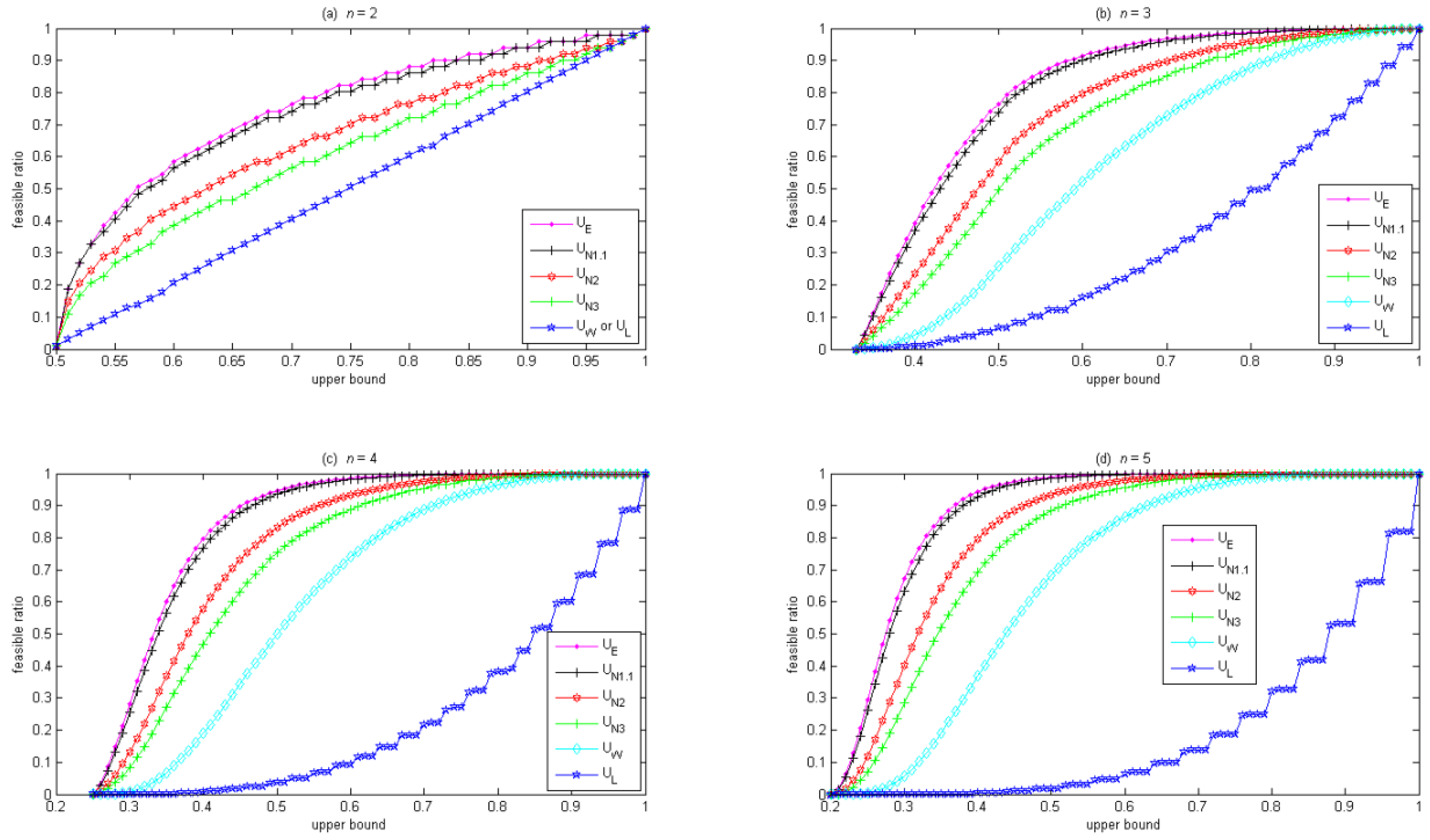
Figure 1 shows that the feasible ratio increases with the upper bound of a diversity constraint in the canonical form. For the weight lower-bound constraint in Equation (8), Figure 1a shows that, given the same upper bound, larger n could have a smaller feasible ratio. Also, as the upper bound gradually decreases from 1 to $\frac{1}{n}$, the feasible ratio reduces quickly at first but slowly afterward (with the exception at n = 2, where the feasible ratio reduces at a constant rate). In contrast, for the rest of the diversity constraints, Figure 1b–f shows that, given the same upper bound, the feasible ratio is always larger for larger n. Also, as the upper bound gradually decreases from 1 to $\frac{1}{n}$, the feasible ratio reduces slowly at first and quickly afterward (with the exception of the weight upper-bound constraint in Equation (3) at n = 2, where the feasible ratio reduces at a constant rate).

Figure 2 compares how these diversity constraints affect the feasible ratio, where the horizontal axis is the upper bound in these diversity constraints, and the vertical axis is the feasible ratio. Given the same upper bound, the ordering of the feasible ratio is: entropy constraint in Equation (10) ≥ L^1.1-norm constraint in Equation (9) ≥ L²-norm constraint in Equation (9) ≥ L³-norm constraint in Equation (9) ≥ weight upper-bound constraint in Equation (3) ≥ weight lower-bound constraint in Equation (8). When the upper bound is 1, the feasible ratio is 1 for all of these diversity constraints. When the upper bound is $\frac{1}{n}$, the feasible ratio approaches 0 for all of these diversity constraints since all of these diversity constraints shrink the feasible region to only one solution, i.e., the equally-weighted portfolio. Notably, when n = 2, the weight upper-bound constraint in Equation (3) is equivalent to the weight lower-bound constraint in Equation (8), as shown in Figure 2a. Also note that in Figure 2, the curve for the L^p-norm constraint gradually approaches the curve for the entropy constraint as p decreases from 3 to 1.1. The curves for L^1.01-norm and L^1.001-norm constraints are omitted in Figure 2 because they closely overlap with the curve for the entropy constraint.

Figure 1. Feasible ratio vs. upper bound for n = 2 to 5.

Figure 1. Feasible ratio vs. upper bound for n = 2 to 5.

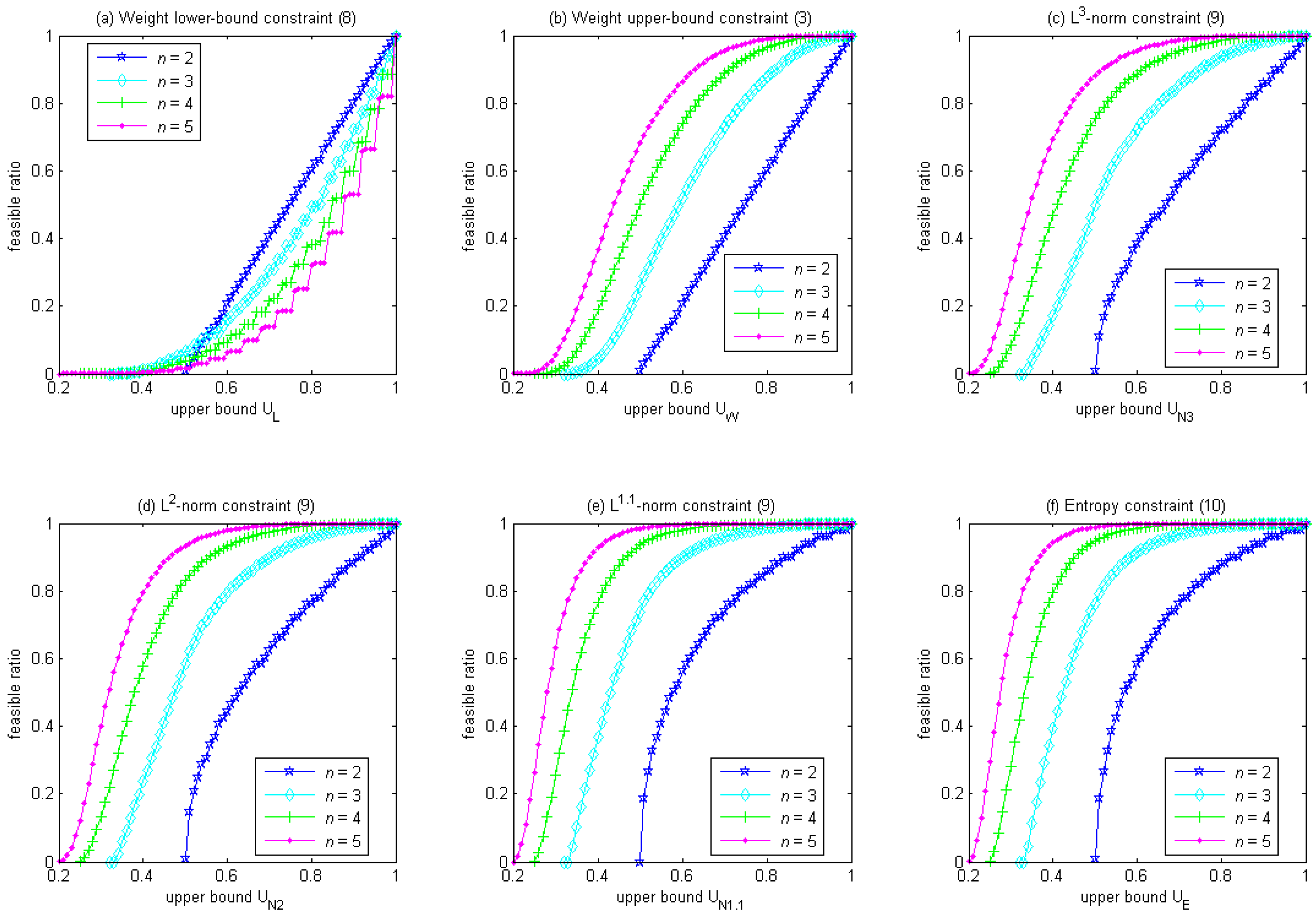
Figure 2. Comparison of feasible ratio for various diversity constraints.

Figure 2. Comparison of feasible ratio for various diversity constraints.

Figure 3. Distribution of the values of $\max (\mathbf{w}), \mathrm{L}(\mathbf{w}),{\mathrm{N}}_3(\mathbf{w}),{\mathrm{N}}_2(\mathbf{w}),{\mathrm{N}}_{1.1}(\mathbf{w})$ and $\mathrm{F}(\mathbf{w})$ in the feasible region of Problem 1 with n = 3.

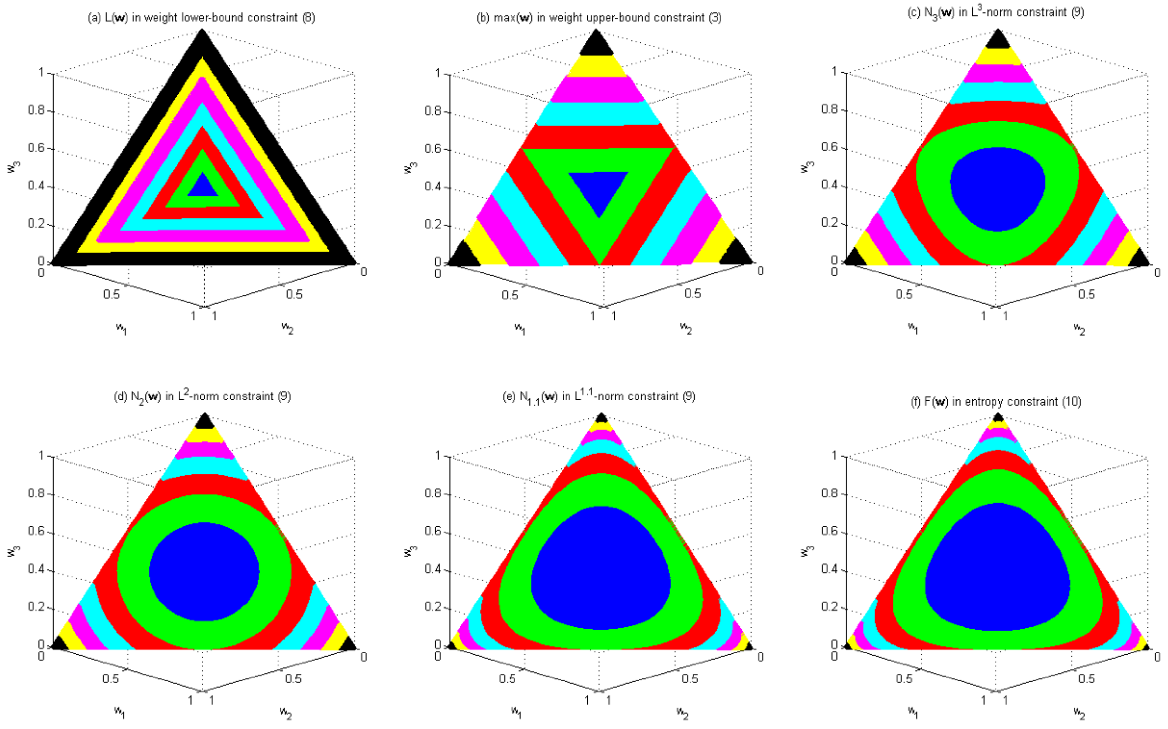
Figure 3. Distribution of the values of $\max (\mathbf{w}), \mathrm{L}(\mathbf{w}),{\mathrm{N}}_3(\mathbf{w}),{\mathrm{N}}_2(\mathbf{w}),{\mathrm{N}}_{1.1}(\mathbf{w})$ and $\mathrm{F}(\mathbf{w})$ in the feasible region of Problem 1 with n = 3.

Figure 3 illustrates how these diversity constraints change the shape of the feasible region of Problem 1 with n = 3. The original feasible region of Problem 1 with n = 3 is the region enclosed by the largest triangle in each subfigure of Figure 3. Figure 3 shows how the values of $\max (\mathbf{w}), \mathrm{L}(\mathbf{w}),{\mathrm{N}}_3(\mathbf{w}),{\mathrm{N}}_2(\mathbf{w}),{\mathrm{N}}_{1.1}(\mathbf{w})$ and $\mathrm{F}(\mathbf{w})$ vary within this feasible region, where different colors are used to indicate the values of these functions. Colors blue, green, red, cyan, magenta, yellow and black represent the intervals (0.3, 0.4], (0.4, 0.5], (0.5, 0.6], (0.6, 0.7], (0.7, 0.8], (0.8, 0.9] and (0.9, 1.0], respectively.

Figure 3a shows that the weigh lower-bound constraint in Equation (8) results in a feasible region similar to the original feasible region, both in terms of shape and orientation. This property has the potential of gradually excluding the solutions along the border of the feasible region as the upper bound of the constraint decreases.

Figure 3b shows that the weigh upper-bound constraint in Equation (3) results in a feasible region similar to the original feasible region in shape but in the opposite orientation. The property has the potential of gradually excluding the solutions near the corners of the feasible region as the upper bound of the constraint decreases.

Figure 3c–e, respectively, shows that the L³-norm constraint, the L²-norm constraint and the L^1.1-norm constraint result in a feasible region similar to those in Figure 3b, except that the shape of the feasible region becomes a squeezed circle for the L³-norm constraint, a circle for the L²-norm constraint, and a bloated circle for the L^1.1-norm constraint, instead of a triangle in the weight upper-bound constraint. Thus, they all have the potential of gradually excluding the solutions near the corners of the feasible region as the upper bound of the constraint decreases. Given the same upper bound, they all result in a smaller feasible region than the weight upper-bound constraint does. Furthermore, the feasible region of the L³-norm constraint is smaller than that of the L²-norm constraint, which in turn is smaller than that of the L^1.1-norm constraint.

Figure 3f shows that the entropy constraint in Equation (10) results in a feasible region similar to the original feasible region in orientation but different in shape. Similar to Figure 3a, constraint in Equation (10) has the potential of gradually excluding the solutions along the border of the feasible region as the upper bound of the constraint decreases. Given the same upper bound, constraint in Equation (10) results in a feasible region larger than any of the previous five constraints does. Notably, the feasible region of the L^1.1-norm constraint is similar to that of constraint in Equation (10).

6. Conclusions

Diversity constraints are often used in the portfolio optimization problem to avoid overly concentrated portfolios. Previous work has shown that diversity constraints improve the performance of the portfolio optimization problem. However, no comparison among the diversity constraints for the portfolio optimization problem has been conducted. In this paper, we review the commonly-used diversity constraints in the literature, and show that their differences on both their forms (i.e., upper or lower bound) and the ranges of their bounds make it difficult to compare them systematically. A canonical form of the diversity constraints is proposed to resolve this problem. Using the canonical form, we can compare these diversity constraints at the same upper bound. Our analytical results show that the weight lower-bound constraint in Equation (8) is the strictest at enforcing diversity, and consequently results in the smallest feasible region. The weight upper-bound constraint in Equation (3) comes second. The L^p-norm constraint in Equation (9) offers different level of diversity control by using different values for p. Although the entropy constraint in Equation (10) appears to be the loosest at enforcing diversity among the diversity constraints analyzed in Section 5, the L^p-norm constraint with p approaching 1 shows similar results to that of the entropy constraint in Equation (10). By transforming these diversity constraints into the canonical form, we show that, these diversity constraints at the same upper bound exhibit a subset relation among their feasible regions.

In addition to allowing systematic comparison among these diversity constraints, the canonical form also eases the task of choosing the upper-bound value for a diversity constraint. In practice, the meaning of the bound for the weight upper/lower bound constraint is easy to understand by the investors. However, without the canonical form, setting a threshold on either the entropy or the L^p-norm of the weighted vector w of a portfolio, as did in Equations (5) and (6), is less intuitive than setting a bound on the weights. With the canonical form, the upper bound of a diversity constraint is always restricted to the interval $[\frac{1}{n},1]$, which is the same as the range of the upper bound for the weight upper-bound constraint in Equation (3). Therefore, the investors can choose the value for the upper bound from the same range, regardless which diversity constraint is used.

References

- Markowitz, H. Portfolio selection. J. Finan. 1952, 7, 77–91. [Google Scholar]
- Usta, I.; Kantar, Y.M. Mean-variance-skewness-entropy measures: A multi-objective approach for portfolio selection. Entropy 2011, 13, 117–133. [Google Scholar] [CrossRef]
- Huang, X.X. Portfolio Analysis from Probabilistic to Credibilistic and Uncertain Approaches; Springer: Berlin/Heidelberg, Germany, 2010. [Google Scholar]
- DeMiguel, V.; Garlappi, L.; Uppal, R. Optimal versus naive diversification: How inefficient is the 1/N portfolio strategy? Rev. Financ. Stud. 2009, 22, 1915–1953. [Google Scholar] [CrossRef]
- Best, M.J.; Grauer, R.R. On the sensitivity of mean-variance-efficient portfolios to changes in asset means: Some analytical and computational results. Rev. Financ. Stud. 1991, 4, 315–342. [Google Scholar] [CrossRef]
- Best, M.J.; Grauer, R.R. Sensitivity analysis for mean-variance portfolio problems. Manage. Sci. 1991, 37, 980–989. [Google Scholar] [CrossRef]
- Green, R.C.; Burton, H. When will mean-variance efficient portfolios be well diversified? J. Finan. 1992, 47, 1785–1809. [Google Scholar] [CrossRef]
- Frost, P.A.; Savarino, J.E. For better performance: Constrain portfolio weights. J. Portfolio Manag. 1988, 15, 29–34. [Google Scholar] [CrossRef]
- DeMiguel, V.; Garlappi, L.; Nogales, F.J.; Uppal, R. A generalized approach to portfolio optimization: Improving performance by constraining portfolio norms. Manag. Sci. 2009, 55, 798–812. [Google Scholar] [CrossRef]
- Huang, X.X. An entropy method for diversified fuzzy portfolio selection. Int. J. Fuzzy Syst. 2012, 14, 160–165. [Google Scholar]
- Jagannathan, R.; Ma, T.S. Risk reduction in large portfolios: Why imposing the wrong constraints helps. J. Financ. 2003, 58, 1651–1683. [Google Scholar] [CrossRef]
- Hlouskova, J.; Lee, G.S. Legal restrictions on portfolio holdings: Some empirical results; Reihe Ökonomie / Economics Series, Institut für Höhere Studien (IHS) 93. Institute for Advanced Study: Vienna, Austria, 2001. Available online: http://hdl.handle.net/10419/71204 (accessed on 25 October 2013).
Appendix. Proofs of Corollaries and Auxiliary Lemmas
Lemma 9.
If
is a feasible solution of Problem 1, then .
Proof.
Without loss of generality, let
and . The constraint in Equation (8) yields . Since , we have
and consequently
by the constraint in Equation (2). Therefore,
holds. □
Proof of Corollary 1.
Let
be a feasible solution of Problem 2, then . Lemma 9 yields , and . Thus,
must be a feasible solution of Problem 3. □
Lemma 10.
is a feasible solution of Problem 1, then
for any .
Without loss of generality, let . Equations (9) and (2) yield
By ,
and constraint (1),
holds for all . Consequently, . Finally, ,
and
yield . □
Proof of Corollary 2.
be a feasible solution of Problem 3, then . Lemma 10 yields
for any . Thus,
must be a feasible solution of Problem 4.
Lemma 11.
Equations (9) and (2) yield , and =. Thus, . Therefore,
holds. Since
and ,
must hold.
Proof of Corollary 3.
be a feasible solution of Problem 4a, then . Lemma 11 yields , and consequently . Thus,
must be a feasible solution of Problem 4b.
Lemma 12.
Without loss of generality, let . Constraint (2) yields . Then,
yields
for all . Thus, , and consequently, .
Proof of Corollary 4.
be a feasible solution of Problem 3, then . Lemma 12 yields , and consequently . Thus,
must be a feasible solution of Problem 5.
© 2013 by the authors; licensee Molecular Diversity Preservation International, Basel, Switzerland. This article is an open access article distributed under the terms and conditions of the Creative Commons Attribution license (http://creativecommons.org/licenses/by/3.0/).
Share and Cite
MDPI and ACS Style
Lin, J.-L. On the Diversity Constraints for Portfolio Optimization. Entropy 2013, 15, 4607-4621. https://doi.org/10.3390/e15114607
AMA Style
Lin J-L. On the Diversity Constraints for Portfolio Optimization. Entropy. 2013; 15(11):4607-4621. https://doi.org/10.3390/e15114607
Chicago/Turabian StyleLin, Jun-Lin. 2013. "On the Diversity Constraints for Portfolio Optimization" Entropy 15, no. 11: 4607-4621. https://doi.org/10.3390/e15114607