Article

Law of Multiplicative Error and Its Generalization to the Correlated Observations Represented by the q-Product

Graduate School of Advanced Integration Science, Chiba University, 1-33 Yayoi, Inage, Chiba,Chiba 263-8522, Japan
Entropy 2013, 15(11), 4634-4647; https://doi.org/10.3390/e15114634
Submission received: 8 September 2013 / Revised: 6 October 2013 / Accepted: 21 October 2013 / Published: 28 October 2013
(This article belongs to the Collection Advances in Applied Statistical Mechanics)

Abstract

:
The law of multiplicative error is presented for independent observations and correlated observations represented by the q-product, respectively. We obtain the standard log-normal distribution in the former case and the log-q-normal distribution in the latter case. Queirós’ q-log normal distribution is also reconsidered in the framework of the law of error. These results are presented with mathematical conditions to give rise to these distributions.

1. Introduction

In physics, especially in thermodynamics, statistical physics and quantum physics, fluctuation of a physical observable has been significant for describing many physical phenomena [1]. There are many theoretical ways to unify fluctuations, such as the Boltzmann equation, the maximum entropy principle, the Fokker-Planck equation, and so on. In every approach, fluctuation is considered as a variance of values of a physical observable. In repeated measurements of a physical observable, the most natural and simplest assumption is the “independence” of the measurements. This corresponds to the treatment in Boltzmann-Gibbs-Shannon statistics, i.e., every value of a physical quantity is observed independently in repeated measurements [2]. On the other hand, in generalized statistics, such as Tsallis statistics, a certain correlation as a generalized independence (e.g., the “q-product” in Tsallis statistics) is applied. In fact, starting from the q-product, Tsallis entropy is uniquely determined as the corresponding entropy [3]. In order to unify and determine probability distributions of physical values for each of the statistics, the most simple and powerful way is the reformulation of the “law of error” because the standard product as independence (which appears in the likelihood function) in Boltzmann-Gibbs-Shannon statistics is only replaced by the generalized product in generalized statistics. Note that the “error” in the law of error means “fluctuation” in physics.
The law of error is well known as the first derivation of the normal distribution by Carl F. Gauss, so that, nowadays, the normal distribution is also called Gaussian distribution [4,5]. Gauss’ contribution on this topic is not only his discovery of the important probability distribution, but it is also the first application of the likelihood function in his discovery, although it might be intuitive. Later, the likelihood function was fully understood by Ronald A. Fisher [6], the pioneer of modern statistics wherein the maximum likelihood estimation plays an important role [7]. Gauss’ derivation is now considered a typical application of the maximum likelihood method. Moreover, Gauss’ law of error has often been taken as an assumption of error in most of the fields related to measurement.
In the original Gauss’ law of error, an observed value is given by the addition of an error to the true value. We call this type of error “additive error”, which is the most fundamental and natural type in our understanding. An error is a difference between an observed value and the true value, so other types of error such as the ratio can be also considered. In this paper, a “multiplicative error”, given by the ratio of an observed value and the true value, is applied to the formulation of the law of error. As a result, a multiplicative error is found to follow a log-normal distribution, which is quite a natural derivation of a log-normal distribution with fruitful backgrounds in the sense that the mathematical condition to obtain a log-normal distribution is clearly presented. Moreover, the original law of error was recently generalized for the so-called q-statistics (i.e., Tsallis statistics [8,9]) by means of the q-product [10,11]. Tsallis statistics describes a strongly correlated system exhibiting power-law behavior, which results in the q-Gaussian distribution as the distribution of an additive error in q-statistics [12]. Along similar lines, the laws of error for other generalized statistics are also presented in [13,14]. The q-Gaussian distribution provides us not only with a one-parameter generalization of the standard Gaussian distribution ( q = 1 ), but also with a nice unification of important probability distributions such as the Cauchy distribution ( q = 2 ), the t-distribution ( q = 1 + 2 n + 1 , n N ) and Wigner semicircle distribution ( q = - 1 ). The q-Gaussian distribution was originally derived from the maximization of Tsallis entropy under the appropriate constraint [15,16], and Tsallis entropy is uniquely determined from the q-multinomial coefficient defined by means of the q-product [3]. Therefore, these mathematical results are consistent with each other, because every mathematical formulation in q-statistics originates in the fundamental nonlinear differential equation d y / d x = y q with the q-exponential function as its solution [17,18,19]. Thus, along these characterizations using the maximum likelihood method, a probability distribution for a multiplicative error in q-statistics is expected, that is, a log-q-normal distribution, with clear mathematical reasons for obtaining this distribution in the framework of the law of error. Note that this paper analytically derives the q-Gaussian distribution and the log-q-normal distribution from the maximum likelihood principle. Relevant important discussions about the numerical verification in q-statistics can be found in [20,21], which is not applicable in the present mathematical work.
This paper consists of five sections. Following this first section, the introduction, Section 2 presents the definition of additive error and multiplicative error for the discussion in this paper. Section 3 derives the law of error for these two types of error in the case of independent observations. Based on the previous sections, Section 4 discusses its generalization for the case of correlated observations represented by the q-product. The final section is devoted to the conclusion.

2. Additive Error and Multiplicative Error

A given observed value, x R , is assumed to have some kinds of error in it. In the original law of error, an additive error is considered in the sense:
x = x ^ + e a
where x ^ is the true value and e a is an additive error. On the other hand, in some fields, a multiplicative error is taken into consideration in the form:
x = e m · x ^
where e m > 0 is a multiplicative error. An alternative expression for a multiplicative error, e m , is sometimes formulated as x = 1 + e m x ^ with 1 + e m > 0 , but for simplicity, we use Equation (2) throughout the paper. In case the true value x ^ = 0 i . e . , x = 0 in Equation (2), obviously, a multiplicative error, e m , is not employed. Due to the positivity of e m , the sign of x and x ^ coincide with each other. When a multiplicative error, e m , is considered, the only case x > 0 i . e . , x ^ > 0 is discussed without loss of generality. Then, Equation (2) is reformed to be
ln x = ln x ^ + ln e m
which has a similar structure to the additive error Equation (1). Therefore, the law of multiplicative error can be formulated in the same way as the case of additive error.
If the true value, x ^ 0 , and both of these two kinds of errors, e a and e m , are considered, an observed value, x, is given in the form:
x = e m x ^ + e a or x = e m ( x ^ + e a ) .
Throughout the paper, the term “observation” is often used, which means “random variable” in the mathematical sense.
Under these preparations, some mathematical definitions are given for our discussion.
Definition 1
Let X i i = 1 , , n be a random variable with value x i R i = 1 , , n , respectively. Then, for random variables, E i a i = 1 , , n , defined by
E i a : = X i - x ^ i = 1 , , n
with a constant x ^ R , each value e i a of E i a is called an additive error and satisfies
e i a = x i - x ^ i = 1 , , n .
Under the same situation as above, if
x ^ X i > 0
for random variables E i m defined by
E i m : = X i x ^ i = 1 , , n ,
each value e i m of E i m is called a multiplicative error and satisfies
e i m = x i x ^ i = 1 , , n .
Note 2 
Due to the positivity of E i m , the sign of X i and x ^ coincide with each other. When a multiplicative error is considered, without loss of generality, only the case X i > 0 is discussed.
Note that, if both of these two errors are considered, each X i is given by
X i = x ^ E i m + E i a or X i = E i m x ^ + E i a i = 1 , , n .
Usually, only observed values, x 1 , x 2 , , x n R , are given, and other values such as x ^ , e i a , e i m are not known in advance (of course!). Thus, under the assumption that observed values include one of the two kinds of error, the probability distribution of each error should be studied.

3. Law of Error for Independent Observations

In this section, let X i i = 1 , , n in Definition 1 be i.i.d. (independent, identically distributed) random variables which means independent and identical observations.

3.1. Additive Error

X 1 , , X n are i.i.d. random variables, so every E i a has the same probability density function, f a . Then, we define the likelihood function for additive error in independent observations.
Definition 3 
Let f a be the probability density function (pdf, for short) for E i a defined by Equation (5). The likelihood function, L a θ , for additive error is defined as a function of a variable, θ, such that
L a θ : = i = 1 n f a x i - θ .
Then, we have the famous theorem which is often referred to as “Gauss’ law of error” [5].
Theorem 4 
If the function L a θ of θ for any fixed x 1 , x 2 , , x n R attains the maximum value at
θ = θ * : = 1 n i = 1 n x i ,
then f a must be a Gaussian pdf:
f a e = 1 2 π σ exp - e 2 2 σ 2 .
In the proof of this theorem, the following lemma plays an essential role.
Lemma 5 
Let φ be a continuous function from R into itself and satisfying that i = 1 n φ e i = 0 for every n N and e 1 , , e n R with i = 1 n e i = 0 . Then, there exists a R , such that φ e = a e .
The proofs of Theorem 4 and Lemma 5 are found in [12].

3.2. Multiplicative Error

In the case of a multiplicative error, the random variables, E i m and X i , and a constant, x ^ , are all positive, so that by taking the logarithm of both sides of (8), we have
ln E i m = ln X i - ln x ^ i = 1 , , n
which is a similar form to (5). The ln E i m are also i.i.d. random variables, so every ln E i m has the same probability density function.
Definition 6 
By means of the random variables, E i m , defined by (8), the new random variables, F i m and Y i , are defined by
F i m : = ln E i m i = 1 , , n ,
Y i : = ln X i i = 1 , , n .
Then, the likelihood function, L m θ , for multiplicative error is defined by
L m θ : = i = 1 n f Y m y i - θ
where f Y m is the pdf of F i m .
Then, we obtain the law of multiplicative error in independent observations.
Theorem 7 
If, for any fixed x 1 , x 2 , , x n R + , the function L m θ attains the maximum value at
θ = θ * : = 1 n i = 1 n ln x i ,
then f Y m must be a Gaussian pdf:
f Y m e = 1 2 π σ exp - e 2 2 σ 2 .
Note that
i = 1 n y i - θ * = i = 1 n ln x i - θ * = 0
which means that Lemma 5 can be applied to the proof of the theorem, which is almost the same as that of Gauss’ law of error.
The pdf, f Y m , is for the random variable F i m = ln E i m , so that the pdf, f X m , for E i m is easily obtained.
Corollary 8 
The pdf, f X m , for the random variable, E i m > 0 , is given by the log-normal distribution:
f X m e = f Y m ln e 1 e = 1 2 π σ e exp - ln e 2 2 σ 2 .

4. Law of Error for Correlated Observations Represented by the q-Product

In the standard maximum likelihood principle, the random variables used in the likelihood function, L θ , are assumed to be independent. Recently, the likelihood function was generalized for correlated systems by means of the q-product and its maximization results in the q-Gaussian distribution which coincides with the probability distribution obtained in the maximization of Tsallis entropy under the appropriate constraint on the variance [12]. The q-Gaussian distribution recovers several typical distributions: Cauchy distribution ( q = 2 ), t-distribution ( q = 1 + 2 n + 1 , n N ), the standard Gaussian distribution ( q = 1 ) and Wigner semicircle distribution ( q = - 1 ). In other words, these distributions belong to a family of q-Gaussian distributions.
The law of multiplicative error for correlated observations will be obtained in this section, following the lines of the derivation in the previous section. For this purpose, the mathematical preliminaries on the q-product are given.
The maximum entropy principle (MaxEnt, for short) for Boltzmann-Gibbs-Shannon entropy:
S 1 : = - f x ln f x d x
yields the exponential function, exp x , which is well known to be characterized by the fundamental linear differential equation d y / d x = y . In parallel with this, the MaxEnt for Tsallis entropy:
S q : = 1 - f x q d x q - 1
yields a generalization of the exponential function, exp q x , [17,19,22] which is characterized by the nonlinear differential equation d y / d x = y q [23] (see also Chapter 10 in [24] for more general deformations). According to the solution of d y / d x = y q , the q-logarithm ln q x and the q-exponential exp q x are defined as follows:
Definition 9 
The q-logarithm ln q x : R + R and the q-exponential exp q x : R R are defined by
ln q x : = x 1 - q - 1 1 - q ,
exp q x : = 1 + 1 - q x 1 1 - q if 1 + 1 - q x > 0 , 0 otherwise.
Then, a new product, q , to satisfy the following identities as the q-exponential law is introduced.
ln q x q y = ln q x + ln q y ,
exp q x q exp q y = exp q x + y .
For this purpose, the new multiplication operation, q , is introduced in [10,11]. The concrete forms of the q-logarithm and q-exponential are given in Equation (24) and Equation (25), so that the above requirement, Equation (26) or (27), as the q-exponential law leads to the definition of q between two positive numbers.
Definition 10 
For x , y R + , if x 1 - q + y 1 - q - 1 > 0 , the q-product q is defined by
x q y : = x 1 - q + y 1 - q - 1 1 1 - q .
The q-product recovers the standard product in the sense lim q 1 x q y = x y . The fundamental properties of the q-product q are almost the same as the standard product, but
a x q y a x q y a , x , y R .
The other properties of the q-product are available in [10,11].
Note that, in general, the maximization of some general entropies such as Rényi entropy yields the same q-exponential function. Contrary to the procedure in the MaxEnt, starting from the q-exponential function and the q-product, Tsallis entropy is uniquely determined, which means that the entropy corresponding to the q-exponential function is only Tsallis entropy in the mathematically consistent sense. See [3,19] for these approaches.
In this section, let X i i = 1 , , n in Definition 1 be identically distributed random variables.

4.1. Additive Error

X 1 , , X n are identical random variables, so every E i a has the same pdf f a . Then, we define the q-likelihood function, L q a θ , for additive error in the correlated observations.
Definition 11 
Let f a be the pdf for E i a defined by Equation (5). The q-likelihood function L q a θ for additive error is defined by
L q a θ : = f a x 1 - θ q q f a x n - θ .
Theorem 12 
If the function, L q a θ , of θ for any fixed x 1 , x 2 , , x n R attains the maximum value at
θ = θ * : = 1 n i = 1 n x i ,
then f a must be a q-Gaussian pdf:
f a e = 1 Z q exp q - β e 2
with β > 0 and where
Z q : = d e exp q - β e 2 .
The proof of the theorem is found in [12].
Using the so-called q-variance, σ 2 , β and Z q are represented by
β = 1 3 - q σ 2 ,
Z q = 3 - q q - 1 σ 2 1 2 B 3 - q 2 q - 1 , 1 2 1 < q < 3 3 - q 1 - q σ 2 1 2 B 2 - q 1 - q , 1 2 q < 1
where B is the beta function.
The q-Gaussian pdf can also be derived by using the standard product (independence) and the general error, e θ (defined further on), instead of the q-product in Equation (30).
Theorem 13 
If the likelihood function:
L g θ : = i = 1 n f e x i - θ
for any fixed x 1 , x 2 , , x n attains the maximum value at
θ = θ * such that i = 1 n e x i - θ * = 0
where
e θ : = tan β q - 1 θ β q - 1 , q > 1 θ , q = 1 tan β 1 - q θ β 1 - q , q < 1 and β > 0 ,
then the probability density function, f, must be a q-Gaussian probability density function:
f e exp q - β e 2 .
The meaning of the general error Equation (38) is still missing at present. The proof of this theorem is found in the Appendix.

4.2. Multiplicative Error

Similar to above, the ln E i m defined by Equation (14) are identical random variables, so every ln E i m has the same pdf.
Definition 14 
Given the random variables, F i m and Y i , defined by Equations (15) and (16), respectively, the q-likelihood function, L q m , for a multiplicative error is defined by
L q m θ : = f Y m y 1 - θ q q f Y m y n - θ
where f Y m is the pdf of F i m .
Theorem 15 
If the function, L q m θ , for any fixed x 1 , x 2 , , x n R attains the maximum value at
θ = θ * : = 1 n i = 1 n ln x i ,
then f Y m must be a q-Gaussian pdf:
f Y m e = 1 Z q exp q - β e 2 .
As expected, f Y m is the pdf for F i m = ln E i m , so that the pdf, f X m , for E i m is easily obtained.
Corollary 16 
The pdf, f X m , for the random variable E i m > 0 is given by
f X m e = f Y m ln e 1 e = 1 Z q · e exp q - β ln e 2 .
Here, the support of f X m is
x > 0 , q > 1 , exp - 1 β 1 - q < x < exp 1 β 1 - q , q < 1 .
We call this distribution Equation (43) “log-q-normal distribution” in contrast to “q-log-normal distribution” given by Queirós, discussed in the next section. The graphs of the log-q-normal distribution are given in Figure 1.
Figure 1. Log-q-normal distribution (q = 0.2, 1.0, 1.8) (linear-linear scale (upper), log-linear (center), log-log scale (lower)).
Entropy 15 04634 g001

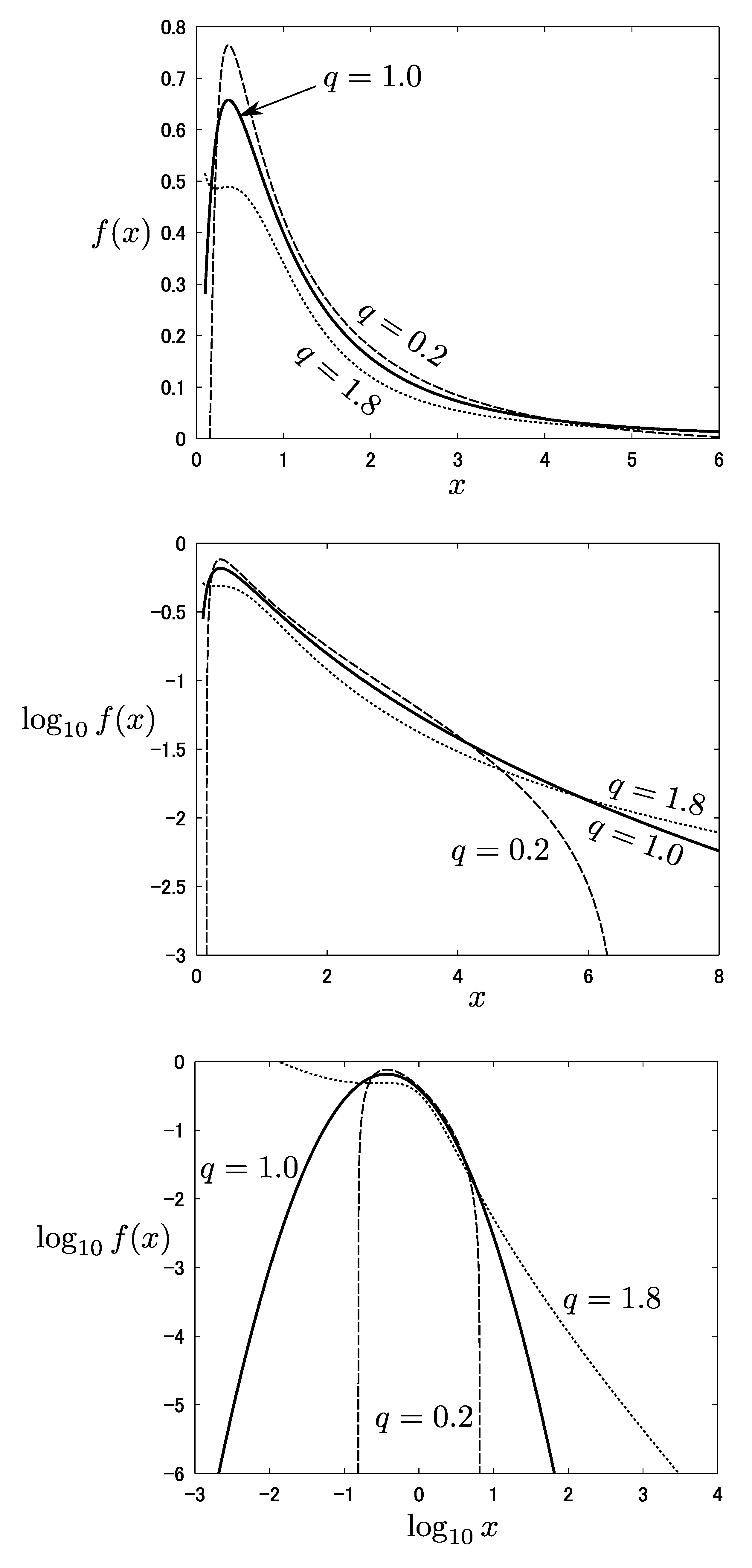
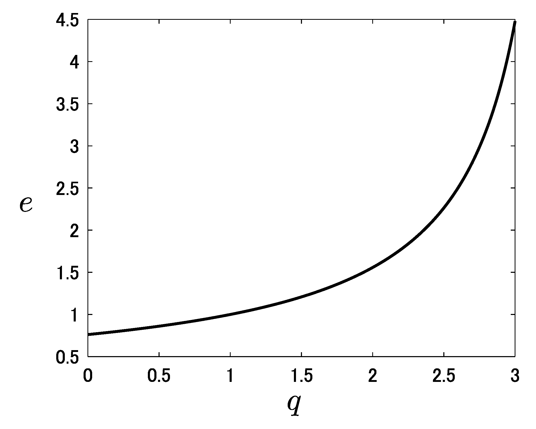
4.3. Reconsideration of Queirós’ q-Log-Normal Distribution in the Framework of the Law of Error

In advance of the present work, Queirós derived the q-log-normal distribution [25,26]:
f q Queirós e = 1 2 π σ e q exp - ln q e 2 2 σ 2
where μ = 0 in his original distribution: 1 2 π σ e q exp - ln q e - μ 2 2 σ 2 . In the framework of the law of error, this distribution can be derived under the following conditions:
  • independent observations, i.e., X i i = 1 , , n are i.i.d. random variables,
  • multiplicative error Equation (2) is modified to
    x = e m q x ^ .
    i.e., the standard logarithm in Equation (14) is replaced by the q-logarithm:
    ln q E i m = ln q X i - ln q x ^ i = 1 , , n .
Equation (46) obviously differs from the original multiplicative error Equation (2). Using the q-logarithm, Equation (46) is reformulated to
ln q x e m = ln q x ^ e m 1 - q
which reveals a scaling by means of e m . This scaling effect disappears when q = 1 . However, at present, a satisfactory explanation of Equation (46) is missing in the law of error, but an interesting interpretation may be found in some physical models.
If Equation (46) is accepted as a modified multiplicative error, the pdf obtained from the similar maximum likelihood method is
f q , q e = 1 Z q · e q exp q - ln q e 2 3 - q σ 2
where Equation (35) is used. We can call this distribution “q-log- q -normal distribution” or“ q , q -log-normal distribution”. This is the most general form of the standard log-normal distribution in the framework of the law of error. Of course, such a general pdf recovers more data than the standard case. The condition giving rise to this general distribution are
  • The likelihood function of identical random variables X i i = 1 , , n is given by the q -product of its pdf,
  • Instead of Equation (2), a modified multiplicative error Equation (46) is obtained.

5. Conclusions

Along the generalization of the law of additive error [12], the law of multiplicative error is presented in the case of independent and correlated observations, respectively. As a result, the standard log-normal distribution and log-q-normal distribution are determined with mathematical conditions to give rise to these distributions. Furthermore, Queirós’ q-log normal distribution is reconsidered in the framework of the law of error.
The law of error is a direct application of the maximum likelihood principle, so that the study on this topic can be applied not only in error analysis or assumptions in practical science such as engineering and experimental physics, but also in statistical inference and divergence theory in theoretical science such as mathematics and theoretical physics.

Acknowledgments

The author is grateful to Jan Naudts for his kind hospitality during the sabbatical stay in the University of Antwerp in 2013, where the present work was done. Comments by Tatsuaki Wada and Ben Anthonis after submission were helpful for improving the present paper. The author would also like to thank the anonymous referee for pointing out the references [20,21]. This work was supported by JSPS KAKENHI, Grant Number 25540106.

Conflict of Interest

The author declares no conflict of interest.

Appendix: Proof of Theorem 13

Proof. 
By taking the derivative of the log-likelihood function L g θ in Equation (36) with respect to θ leads to
d L g d θ L g θ = i = 1 n d f d e · d e x i - θ d θ f e x i - θ .
When θ = θ * , the likelihood function L g θ attains the maximum value, so that
d L g d θ L g θ θ = θ * = 0 if and only if i = 1 n d f d e · d e x i - θ d θ θ = θ * f e x i - θ * = 0 .
Let ρ be defined by
ρ e x - θ * : = d f d e · d e x - θ d θ θ = θ * f e x - θ * ,
then Equation (51) can be rewritten as
i = 1 n ρ e x i - θ * = 0 .
With this, our problem is reduced to determining the function, ρ, satisfying Equation (53) under the constraint Equation (37). By means of Lemma 5, we have
ρ e = a e
for a R . Thus,
d f d e · d e x - θ d θ f e = a e ,
that is,
d f d e · d e θ d θ f e = - a e .
From Equation (38) follows
d d θ e = 1 + q - 1 β e 2 ,
so that Equation (55) becomes
d f d e f e = - a e 1 + q - 1 β e 2 .
The solution, f, satisfying Equation (58) can be obtained as a q-Gaussian pdf:
f e = 1 Z q exp q - β e 2 .
Figure 2. e as a function of q β = θ = 1 .
Entropy 15 04634 g002
The general error, e θ , defined by Equation (38), is obtained as the solution of the differential Equation (57). The graph of e as a function of q is given in Figure 2.

References

  1. Tolman, R.C. The Principles of Statistical Mechanics; Dover: New York, NY, USA, 1938. [Google Scholar]
  2. Lavenda, B.H. Statistical Physics: A Probabilistic Approach; Wiley: New York, NY, USA, 1991. [Google Scholar]
  3. Suyari, H. Mathematical structures derived from the q-multinomial coefficient in Tsallis statistics. Physica A 2006, 368, 63–82. [Google Scholar] [CrossRef]
  4. Gauss, C.F. Theoria Motus Corporum Coelestium in Sectionibus Conicis Solem Ambientium; Perthes: Hamburg, German, 1809; (translation with appendix by Davis, C.H. Theory of the Motion of the Heavenly Bodies Moving About the Sun in Conic Sections; Dover: New York, NY, 1963.). [Google Scholar]
  5. Hald, A. A History of Mathematical Statistics From 1750 to 1930; Wiley: New York, NY, USA, 1998. [Google Scholar]
  6. Fisher, A.R. On the mathematical foundations of theoretical statistics. Philos. Trans. Roy. Soc. A, 1922, 222, 309–368. [Google Scholar] [CrossRef]
  7. Casella, G.; Berger, R.L. Statistical Inference, 2nd ed.; Cengage Learning: Stamford, CA, USA, 2001. [Google Scholar]
  8. Tsallis, C. Possible generalization of Boltzmann-Gibbs statistics. J. Stat. Phys. 1988, 52, 479–487. [Google Scholar] [CrossRef]
  9. Tsallis, C. Introduction to Nonextensive Statistical Mechanics: Approaching a Complex World; Springer: New York, NY, USA, 2009. [Google Scholar]
  10. Nivanen, L.; le Mehaute, A.; Wang, Q.A. Generalized algebra within a nonextensive statistics. Rep. Math. Phys. 2003, 52, 437–444. [Google Scholar] [CrossRef]
  11. Borges, E.P. A possible deformed algebra and calculus inspired in nonextensive thermostatistics. Physica A 2004, 340, 95–101. [Google Scholar] [CrossRef]
  12. Suyari, H.; Tsukada, M. Law of error in Tsallis statistics. IEEE Trans. Inform. Theory 2005, 51, 753–757. [Google Scholar] [CrossRef]
  13. Wada, T.; Suyari, H. κ-generalization of Gauss’ law of error. Phys. Lett. A 2006, 348, 89–93. [Google Scholar] [CrossRef]
  14. Scarfone, A.M.; Suyari, H.; Wada, T. Gauss’ law of error revisited in the framework of Sharma-Taneja-Mittal information measure. Centr. Eur. J. Phys. 2009, 7, 414–420. [Google Scholar] [CrossRef]
  15. Tsallis, C.; Levy, S.V.F.; Souza, A.M.C.; Maynard, R. Statistical-mechanical foundation of the ubiquity of Lévy distributions in nature. Phys. Rev. Lett. 1995, 75, 3589–3593. [Google Scholar] [CrossRef] [PubMed]
  16. Prato, D.; Tsallis, C. Nonextensive foundation of Levy distributions. Phys. Rev. E 1999, 60, 2398–2401. [Google Scholar] [CrossRef]
  17. Tsallis, C. What are the numbers that experiments provide? Quimica Nova 1994, 17, 468. [Google Scholar]
  18. Tsallis, C. What should a statistical mechanics satisfy to reflect nature? Physica D 2004, 193, 3–34. [Google Scholar] [CrossRef]
  19. Suyari, H.; Wada, T. Scaling Property and the Generalized Entropy Uniquely Determined by a Fundamental Nonlinear Differential Equation. In Proceedings of the 2006 International Symposium on Information Theory and its Applications, COEX, Seoul, Korea, 29 October 2006.
  20. Hilhorst, H.J.; Schehr, G. A note on q-Gaussians and non-Gaussians in statistical mechanics. J. Stat. Mech. 2007, P06003. [Google Scholar] [CrossRef]
  21. Dauxois, T. Non-Gaussian distributions under scrutiny. J. Stat. Mech. 2007, N08001. [Google Scholar] [CrossRef]
  22. Tsallis, C.; Mendes, R.S.; Plastino, A.R. The role of constraints within generalized nonextensive statistics. Physica A 1998, 261, 534–554. [Google Scholar] [CrossRef]
  23. Tsallis, C. What should a statistical mechanics satisfy to reflect nature? Physica D 2004, 193, 3–34. [Google Scholar] [CrossRef]
  24. Naudts, J. Generalised Thermostatistics; Springer: London, UK, 2011. [Google Scholar]
  25. Queirós, S.M.D. Generalised cascades. Braz. J. Phys. 2009, 39, 448–452. [Google Scholar] [CrossRef]
  26. Queirós, S.M.D. On generalisations of the log-Normal distribution by means of a new product definition in the Kaypten process. Physica A 2012, 391, 3594–3606. [Google Scholar] [CrossRef]

