2.1. Kolmogorov Stochasticity Index: Deterministic Pattern
Let
be a sample set that follows from iid random variables with
probability density function (pdf),
f, and
cumulative distribution function (cdf)
F. The Kolmogorov stochasticity parameter [
15] is:
where
is the empirical cdf of the
N-sample sequence,
x.
Standard approaches for testing random generators are based on binary hypothesis testing (stochastic or not) and focus on the asymptotic properties of when N tends to infinity. In contrast with these approaches, we assume no binary hypothesis, since we will use the heights of to compare textures in terms of their randomness appearances, whatever the values of the stochasticity indices.
Note that for datasets that are stochastic with respect to F (a consequence of the Glivenko-Cantelli theorem). This implies that any x satisfying is non-stochastic with respect to F. For instance, since we are dealing with a dictionary of continuous cdfs, we will say that a constant sequence is deterministic with respect to this dictionary: for such a sequence, the reader can check that , as far as . Furthermore, we have that the presence of a value with large occurrence in a dataset can be qualified as a deterministic pattern, since it impacts, as well, .
The following section addresses the relevance of in pointing out deterministic patterns, in comparison with other stochasticity measures available in the literature.
2.2. The Relevance of the Kolmogorov Stochasticity Parameter in Detecting Deviations From a Specified Distribution
The results presented in this section concern the sensitivity of different stochasticity measures when data with a given stochasticity degree are corrupted with elementary deterministic patterns with increasing sizes.
There are basically two criteria that distinguish stochasticity measures:
- (1)
The norm used, which can be cumulative or uniform;
- (2)
The distribution, which can be specified as pdf or cdf.
Some examples issued from random generator testing are a) the Kolmogorov-Smirnov test [
21], based on the uniform (
) norm and comparing two cdfs in a binary hypothesis testing, b) the chi-squared test [
22], based on the cumulative
norm and comparing two pdfs in a binary hypothesis testing problem.
Let us consider an N-size dataset (texture image for instance) with a stochasticity degree, η, with respect to a given distribution model. Assume that these data are affected by a deterministic pattern in the sense that a proportion, , of the data is set to a constant value, where K is the size of the pattern under consideration. Since a stochasticity measure can be seen as a dissimilarity measure between distribution functions, a relevant stochasticity measure is such that its stochasticity parameter should increases as K increases (the randomness appearance of the texture has decreased).
In the following experiments, a deterministic pattern consisting of the insertion of K occurrences of a fixed value is introduced into datasets, and the relevance of different stochasticity measures is tested when the size K of this pattern increases. These experiments are performed upon the detail wavelet coefficients of textured images. These coefficients are expected to be very small in smooth regions and large in the neighborhood of edges. Increasing the number of null coefficients, if any, by forcing K large coefficients to zero (deterministic pattern) results in smoothing some edges of the image. This implies reducing the intrinsic stochasticity of the data when K increases. A relevant stochasticity measure should depart from the initial stochasticity degree when K increases.
Table 1.
Experimental setup for testing the relevance of the uniform () norm versus the cumulative norm and Kullback-Leibler divergence (KLD) in stochasticity measurements. The quantities involved in the computation of the relative stochasticity value (RSV) are the empirical distribution and the model. cdf: cumulative distribution function.
| For, do: |
| | Compute the wavelet coefficients,
, of the input image. |
| | Introduce a deterministic pattern among the coefficients of a sub-band |
| | | by setting the K largest coefficients to zero (notation: ). |
| | Compute the stochasticity parameters: |
| | | Check the distribution type from the variable “specification” |
| | | Case | specification is “cdf”, then: |
| | | | Compute RSV |
| | | Case | specification is “pdf”, then: |
| | | |
Compute RSV |
| End |
| Compare the measurements obtained: for a relevant stochasticity measure, |
| | RSV is a non-decreasing function of K. |
We consider the experimental setup presented in
Table 1: different combinations between norms (
) and distribution specifications (cdf, pdf) are used for testing stochasticity measures. In this table,
specifically denotes either the
and
norms. The Kullback-Leibler Divergence (KLD) is also used for comparison purposes. The Kullback-Leibler similarity measure between random variables,
and
, having probability distribution functions
and
is defined as:
In addition, if
denotes the wavelet packet coefficients obtained at sub-band
, then
corresponds to the dataset obtained by setting the
K largest values of
to zero. In particular,
.
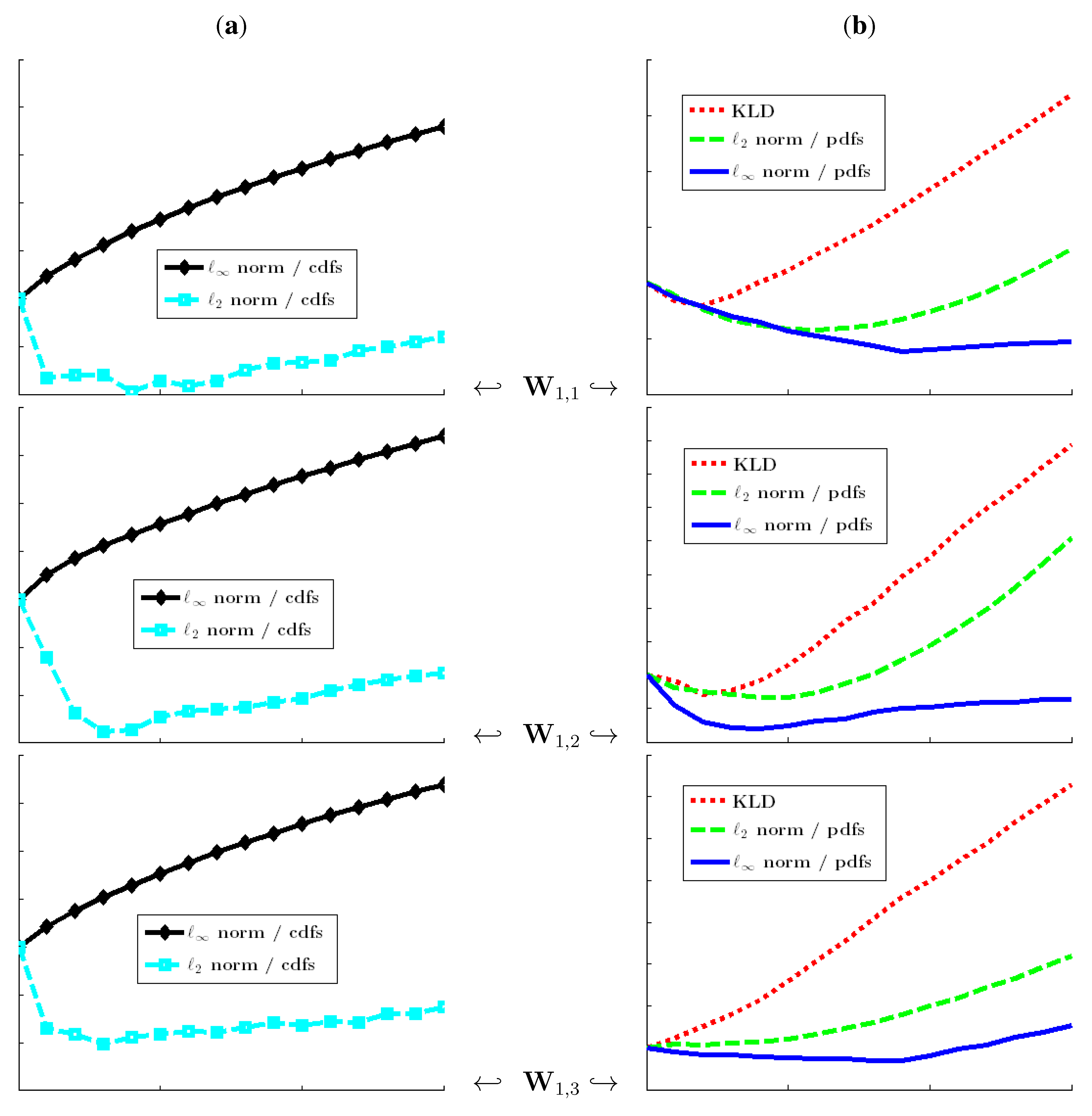
Figure 1.
Relative stochasticity values for the image “Fabric.0004” from the VisTeX database. The RSV of a relevant stochasticity measurement must be an increasing function of the size K of the deterministic pattern. We have and . (a) cdf-based stochasticity measures; (b) pdf-based stochasticity measures.
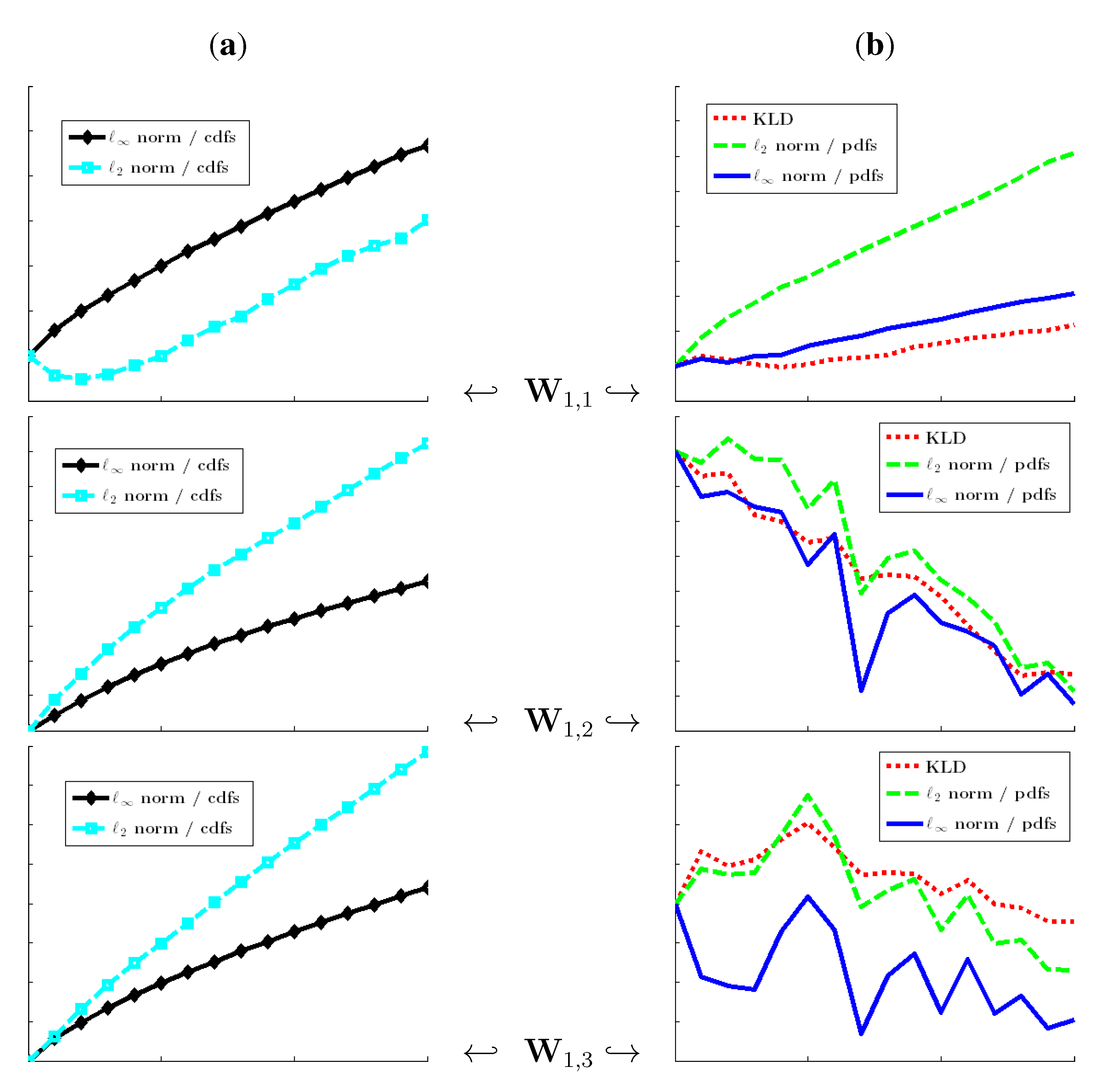
Departure from the initial stochasticity value of the wavelet coefficients is measured with respect to the
generalized Gaussian distributions. In addition, Gaussian, triangle and Epanechnikov kernels have been used for the estimation of the empirical pdfs involved in
Table 1. The results provided in
Figure 1 and
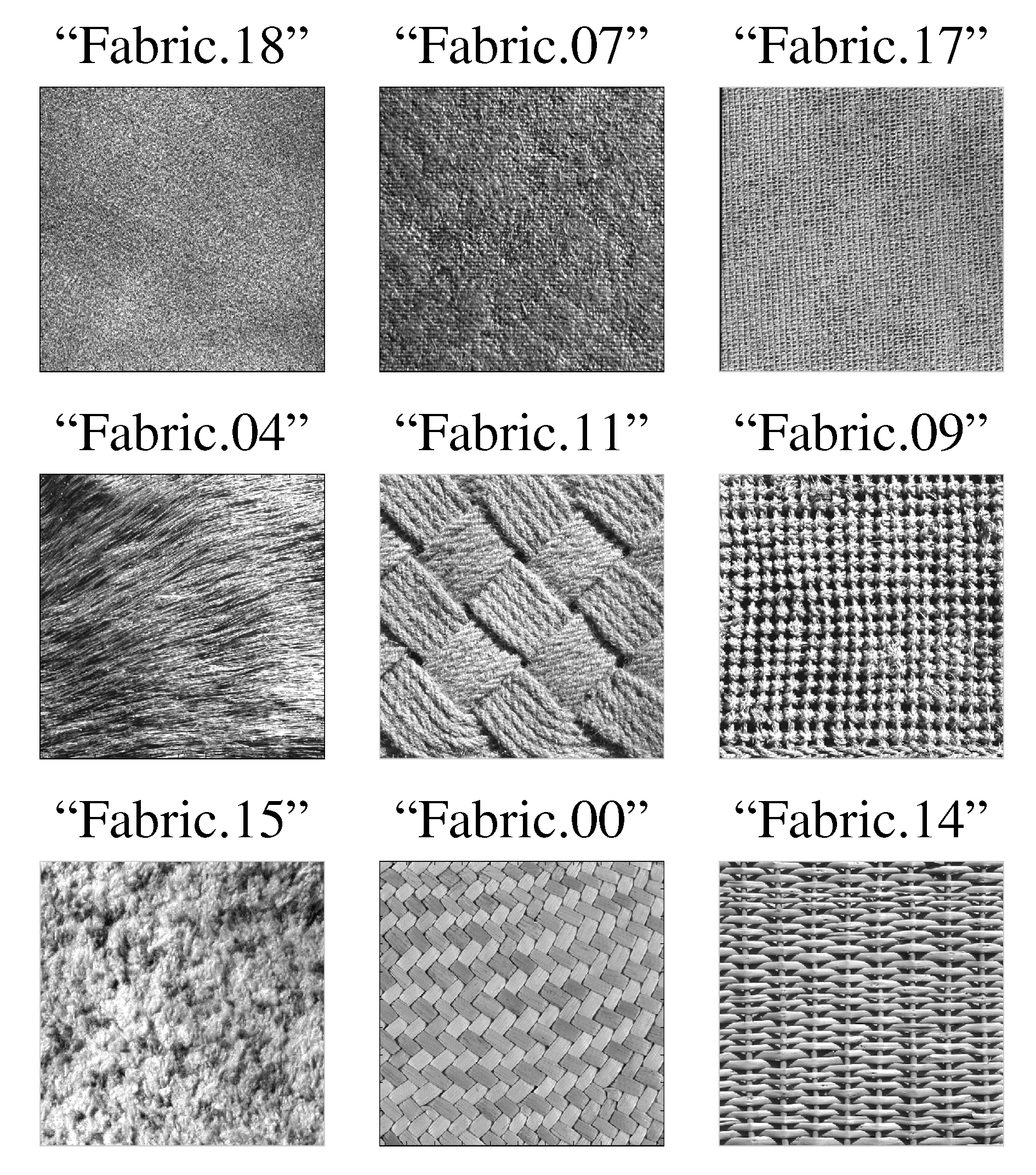
Figure 2 are obtained with a Gaussian kernel, and the wavelet decomposition has been performed with a Daubechies wavelet function of order seven. These results concern the images “Fabric.0004” and “Fabric.0018” from the VisTeX database (see
Figure 1). Results are similar for other textures from the VisTeX database and for other kernels (concerning pdf-based measures).
Figure 2.
Relative stochasticity values for the image “Fabric.0018” from the VisTeX database. The RSV of a relevant stochasticity measurement must be an increasing function of the size K of the deterministic pattern. We have and . (a) cdf-based stochasticity measures; (b) pdf-based stochasticity measures.
As can be seen in
Figure 1 and
Figure 2, the uniform norm on the cdfs (Kolmogorov strategy) is the sole strategy that guarantees a non-decreasing relative stochasticity value (RSV; see
Table 1) when the size
K of the pattern increases. Cumulative measures (
, KLD), as well as pdf-based specifications, are not very relevant for stochasticity assessment, because of non-increasing deviations from the initial stochasticity degree: the local information is blurred through the averaging effect induced by cumulative measures or through neighborhood consideration when computing pdfs. Moreover, the same conclusion as above holds true when the experiments are performed on synthetic random numbers and without the use of wavelet transform.
From now on, we assume that the stochasticity parameter is of the Kolmogorov type: a uniform norm that applies for comparison of the empirical cdf with the distribution model.
Section 3.1 addresses the choice of different bounds on this parameter for generating a semantic stochasticity template. This makes it possible to classify textures by mapping their sequences of stochasticity values on the stochasticity templates under consideration.

