Applications of Entropy in Finance: A Review


School of Economics and Management, Beijing University of Chemical Technology, Beijing 100029, China
*
Author to whom correspondence should be addressed.
Entropy 2013, 15(11), 4909-4931; https://doi.org/10.3390/e15114909
Submission received: 27 September 2013
/
Revised: 20 October 2013
/
Accepted: 30 October 2013
/
Published: 11 November 2013
(This article belongs to the Section Entropy Reviews)
Abstract
:Although the concept of entropy is originated from thermodynamics, its concepts and relevant principles, especially the principles of maximum entropy and minimum cross-entropy, have been extensively applied in finance. In this paper, we review the concepts and principles of entropy, as well as their applications in the field of finance, especially in portfolio selection and asset pricing. Furthermore, we review the effects of the applications of entropy and compare them with other traditional and new methods.
Keywords:
entropy; finance; the principle of maximum entropy; applications; portfolio selection; asset pricingPACS Codes:
89.65.-s Social and economic systems
1. Introduction
The history of the word “entropy” can be traced back to 1865 when the German physicist Rudolf Clausius tried to give a new name to irreversible heat loss, what he previously called “equivalent-value”. The word “entropy” was chosen because in Greek, “en+tropein” means “content transformative” or “transformation content” [1]. Since then entropy has played an important role in thermodynamics. Being defined as the sum of “heat supplied” divided by “temperature” [2], it is central to the Second Law of Thermodynamics. It also helps measure the amount of order and disorder and/or chaos. Entropy can be defined and measured in many other fields than the thermodynamics. For instance, in classical physics, entropy is defined as the quantity of energy incapable of physical movements. Von Neumann used the density matrix to extend the notion of entropy to quantum mechanics. The entropy of a random variable measures uncertainty in probability theory. Entropy quantifies the exponential complexity of a dynamical system, that is, the average flow of information per unit of time in the theory of dynamical systems. In sociology, entropy is the natural decay of structures [3].
Brissaud suggested that entropy could be understood in three aspects [4]: Firstly, in the field of information, entropy represents the loss of information of a physical system observed by an outsider, but within the system, entropy represents countable information. Secondly, entropy measures the degree of freedom. A typical example is gas expansion: the degree of freedom of the position of gas molecules increases with time. Finally, Brissaud believed that entropy is assimilated to disorder. However this conception seems inappropriate to us since temperature is a better measure of disorder.
The application of entropy in finance can be regarded as the extension of the information entropy and the probability entropy. It can be an important tool in portfolio selection and asset pricing.
Philippatos and Wilson were the first two researchers who applied the concept of entropy to portfolio selection [5]. In their thesis, a mean-entropy approach was proposed and compared to traditional methods by constructing all possible efficient portfolios from a randomly selected sample of monthly closing prices on 50 securities over a period of 14 years. They found that the mean-entropy portfolios were consistent with the Markowitz full-covariance and the Sharpe single-index models. Though their research had several drawbacks, they made great contributions to the field of portfolio selection.
Since then many other scholars have enriched the portfolio selection theory with entropy concepts. Some of them have proposed different forms of entropy. More generalized forms of entropy such as the incremental entropy were created. Compared to the traditional portfolio selection theory, the theory based on the incremental entropy emphasized that there was an optimal portfolio for a given probability of return [6]. Some kinds of hybrid entropy were also used in portfolio selection Because the hybrid entropy can measure the risk of securities, some scholars applied the hybrid entropy to the original portfolio selection models. For instance, Xu et al. [7] investigated portfolio selection problems by utilizing the hybrid entropy to estimate the asset risk caused by both randomness and fuzziness. Usta and Kantar [8] tested the mean-variance-skewness-entropy model with the entropy element, which performed better than traditional portfolio selection models in out-of-sample tests. After proposing a mean-variance-skewness model for portfolio selection, Jana et al. [9] added the entropy objective function to generate a well-diversified asset portfolio within optimal asset allocation. Zhang, Liu and Xu developed a possibilistic mean-semivariance-entropy model for multi-period portfolio selection with transaction costs [10]. Zhou et al. formulated a portfolio selection model with the measures of information entropy-incremental entropy-skewness in which the risk of the portfolio was measured by information entropy [11]. Smimoua, Bector and Jacoby considered the derivation of portfolio modeling under a fuzzy situation [12]. Huang proposed a simple method to identify the mean-entropic frontier and developed fuzzy mean-entropy models [13]. Rödder et al. [14] presented a new theory to determine the portfolio weights by a rule-based inference mechanism under both maximum entropy and minimum relative entropy.
Similarly entropy has been applied in option pricing. A typical example is the Entropy Pricing Theory (EPT) introduced by Gulko [15], whose research indicated that the EPT can offer some similar valuation results equal to the Sharpe-Lintner capital asset pricing model and the Black-Scholes formula. He also applied the EPT to stock option pricing [16] and bond option pricing [17]. The EPT model was simple and user-friendly, and its formalism made the Efficient Market Hypothesis operational.
The Principle of Maximum Entropy (MEP) plays an important role in option pricing as well. Back in 1996, Buchen and Kelly [18] used the MEP to estimate the distribution of an asset from a set of option prices. Their research showed that the maximum entropy distribution was able to fit a known probability density function accurately. It could simulate option prices at different strike prices.
Buchen and Kelly’s method had a significant impact. It attracted many others to extend their research and compare all kinds of methods. For example, Neri and Schneider [19] developed a simple robust test for the maximum entropy distribution and tested several samples. They also compared their results to Buchen and Kelly’s. Their methods performed very well both in their two examples from the Chicago Board Options Exchange and they drew the same conclusions as Buchen and Kelly.
Besides the works mentioned above, the maximum entropy method could be used to estimate the implied correlations between different currency pairs [20], to retrieve the neutral density of future stock risks or other asset risks [21], and to infer the implied probability density and distribution from option prices [22,23]. Stutzer and Hawkins [24,25] even used the MEP to price derivative securities such as futures and swaps.
Another useful relevant principle is the Minimum Cross-Entropy Principle (MCEP). In 1951, this principle was developed by Kullback and Leibler [26], and it has been one of the most important entropy optimization principles. In 1996, Buchen and Kelly extended their own research from the MEP to the MCEP [18]. Their results showed that the MCEP has the same effect with the MEP. Four years after Buchen and Kelly’s research, Frittelli discovered sufficient conditions for a unique equivalent martingale measure minimized relative entropy [27]. He also provided a financial interpretation of the minimal entropy martingale measure. The minimal entropy martingale measure could be used in option pricing, which was proved by Benth and Groth [28]. Hunt and Devolder found an explicit characterization of the minimal entropy martingale measure to deal with the market incompleteness [29]. Their model was proved again very useful in empirical implementations. Grandits minimized the Tsallis cross-entropy and told its connection with the minimal entropy martingale measure [30]. In 2004, Branger used the minimum cross-entropy measure to choose a stochastic discount factor (SDF) given a benchmark SDF and to determine the Arrow-Debreu (AD) prices given some sets of benchmark AD prices [31].
The rest of this paper is arranged as follows: some of the major concepts of entropy used in finance are presented in the next section. In Section 3 we review the principles of entropy useful in finance. Section 4 introduces the applications of entropy in portfolio selection. Section 5 is devoted to the applications of entropy in asset pricing, especially in option pricing. Section 6 briefly shows other applications of entropy in finance and the last section concludes.
2. Concepts of Entropy Used in Finance
2.1. The Shannon Entropy
The Shannon entropy [32] of a probability measure on a finite set X is given by:
where and 0 ln 0 = 0.
When dealing with continuous probability distributions, a density function is evaluated at all values of the argument. Given a continuous probability distribution with a density function f(x), we can define its entropy as:
where and f(x)≥0.
2.2. The Tsallis Entropy
For any positive real number α, the Tsallis entropy of order α of a probability measure p on a finite set X is defined as [33]:
Although these entropies are most often named after Tsallis due to his work in the area [33], they had been studied by others long before him. For example, Havrda and Charvát [34] introduced a similar formula in information theory in 1967, and in 1982, Patil and Taillie used Hα as a measure of biological diversity [35]. The characterization of the Tsallis entropy is the same as that of the Shannon entropy except that for the Tsallis entropy, the degree of homogeneity under convex linearity condition is α instead of 1.
2.3. The Kullback Cross-entropy
If we have no other information other than that each and the sum of the probabilities is unity, we have to assume the uniform distribution due to Laplace’s principle of insufficient reasons. It is a special case of the principle of maximum uncertainty according to which the most uncertain distribution is the uniform distribution. In other words, being most uncertain means being most close to the uniform distribution. Therefore we need a measure of the “distance” between two probability distributions: and .
Kullback and Leibler proposed the Kullback cross-entropy which is one of the simplest measures satisfying all of our requirements for distance [26]:
2.4. The Tsallis Relative Entropy
In 1998, Tsallis [36] introduced a generalization of Kullback cross-entropy called the Tsallis relative entropy or q-relative entropy. It is given as:
where is a probability distribution and is a reference distribution. For uniform the Tsallis relative entropy reduces to negative Tsallis entropy , which is described in subsection 2.2 and formula (3).
2.5. The Fuzzy Entropy
Fuzzy entropy is an important research topic in fuzzy set theory. Luca and Termini [37] were the first to define a non-probabilistic entropy with the use of fuzzy theory. Other scholars such as Bhandari and Pal [38], Kosko [39], Pal and Bezdek [40], and Yager [41] have also given their definitions. These entropy definitions are characterized by the uncertainty resulting from linguistic vagueness instead of information deficiency.
Based on credibility, Li and Liu [42,43] proposed a new definition of fuzzy entropy characterized by the uncertainty resulting from the information deficiency due to failing to predict specified values accurately.
A general definition of the expected value of a fuzzy variable ξ with membership function is given as:
where , , and A is any subset of the real numbers R. The function is almost equal to , is also referred to as the possibility distribution of ξ.
Provided that at least one of the two integrals is finite, Equation (6) is a type of Choquet integral. The Choquet integral is usually regarded as the generalization of mathematical expected values in interpreting the measurement theories.
Then, its entropy is defined as:
where with the convention that . and:
when ξ is a continuous fuzzy variable.
If fuzzy variables ξ and η are continuous, the cross-entropy of ξ from η was defined as:
where T: [0,1]×[0,1]→[0,∞) is a binary function defined as .
2.6. Other Kinds of Entropy
There are some other kinds of entropy in literatures including the Rényi entropy, the Havrda–Charvát entropy, the incremental entropy and the Fermi-Dirac information entropy.
The Rényi entropy [44] is defined as follows:
where α > 0 as a constant and p(x) is a probability density.
Consider the prices of N securities in a portfolio as a N-dimension vector and the price of the kth security may have nk values, k = 1,2,…,N. So there are price vectors. We assume that the ith price vector is , current price vector is , and the return from the kth security is rik when the price vector xi happens. is the proportion of investment in the kth security.
Taking its logarithmic value, we have:
We call H(x) “the incremental entropy”, which has the same metric as information. When we value it based on the logarithm value, H(x) means the time needed for capital to double.
For the Fermi-Dirac information entropy:
where B is the asset capacity, and j is the number of the assets, j = 1,2,…,n. For each jth asset aj is the proportion of investment.
2.7. Generalised Entropy
In parts of the mathematics literature, generalized entropy is also called f-divergence [45,46]. Csiszár [47] and Ali and Silvey [48] introduced the f-divergence:
where μ is a σ-finite measure which dominates P and Q. The integrand is specified at the points where the densities and/or are zero.
For , the f-divergence reduces to the classical “information divergence” D(P,Q). For the convex of concave functions f (t) = tα, α > 0, we obtain the so-called Hellinger integrals:
For the convex functions:
we obtain the Hellinger divergences:
which are strictly increasing functions of the Rényi divergences:
3. Principles of Entropy Used in Finance
3.1. Jaynes’ Maximum Entropy Principle
The rationale for the maximum entropy principle can be stated in the following way: out of all the distributions consistent with the constraints, choose the one that [49]:
- (1)
- has the maximum uncertainty; or
- (2)
- is least committed to the information not given to us; or
- (3)
- is most random; or
- (4)
- is most unbiased (any deviation from the maximum entropy results in a bias).
Just as its name implies, its principle is to maximize the entropy given its constraints. So the maximum entropy distribution can be:
subject to
In order to solve the optimization problem in formula (20), the Lagrangian function is applied as below:
where are Lagrange parameters. The Lagrange multipliers are the partial derivatives of with respect to , respectively.
3.2. Kullback’s Minimum Cross-Entropy Principle
As introduced before, the Kullback’s cross-entropy can be considered as an “entropy distance” between the two distributions p(x) and q(x). It is not a true metric distance, but it satisfies S(p,p) = 0 and S(p,q) > 0, whenever p ≠ q. The Principle of Minimum Cross-Entropy (MCEP) states that out of all probability distributions satisfying given constraints, we should choose the one that is closest to the least prejudiced posterior density p(x). This distribution is the Minimum Cross-Entropy Distribution:
This gives us Kullback’s minimum directed divergence or minimum cross-entropy principle. when , we have the following result:
Obviously, Equation (23) shows the relation between the minimum cross-entropy principle and Jaynes’ maximum entropy principle.
4. Applications of Entropy in Portfolio Selection
Markowitz’s mean-variance model [50], which is based on the assumption that returns of assets follow a normal distribution, has been accepted as a pioneer portfolio selection model. However, it often leads to portfolios highly concentrated on a limited number of assets, which deviates from the original purpose of diversification. It also performs poorly in out-of-sample tests. Therefore, for distributions that are asymmetrical or non-normal, a different measure of uncertainty is required, which should be more dynamic and general than the variance, and does not rely on a specific distribution. As entropy is a well-known measure of diversity, many scholars apply it to the portfolio selection theory.
4.1. Entropy as a Measure of Risk
As mentioned in Section 1, Philippatos and Wilson were the first two authors who applied the concept of entropy to portfolio selection [5]. They tried to maximize the expected portfolio return as well as minimize the portfolio entropy in their models. They proposed the concepts of individual entropy (the individual entropy of the security whose return R is discrete random variable with probabilities pi, i = 1,2,…,n, is defined as ), joint entropy (the joint entropy of investment in two securities whose returns R1 and R2 are discrete random variables taking the values R1i, i = 1,2,…,n with probabilities pi, I = 1,2,…,n and R2j, j = 1,2,…,m with probabilities pj, j = 1,2,…,m is defined as where . = the probability that return 1 is in state i and return 2 is in state j) and conditional entropy (the conditional entropy is the marginal entropy gained from the occurrence of an event, R2, given the occurrence of another event R1. The conditional entropy between two security returns is defined as , where = the probability that return 2 is in state i, given that return 1 is in state j. Thus, the joint entropy of two non-independent returns is or .
Given the required individual, joint, and conditional subjective probabilities, they defined the entropy of a single-index portfolio as:
where R1, R2 and R3 are returns of three securities respectively, RI is the return correlated with a market index, Xi is the fraction of funds invested in security i. The portfolio risk can be minimized by minimizing:
Their theory has been proved useful by their empirical results. They randomly selected fifty securities from the New York Stock Exchange and the Dow Jones Industrial Index. Their sample data included monthly closing prices, cash dividends, stock dividends, and stock splits for a fourteen-year period from January 1957 to December 1970. After adjustments for stock dividends and stock splits, the relative return was computed as follows:
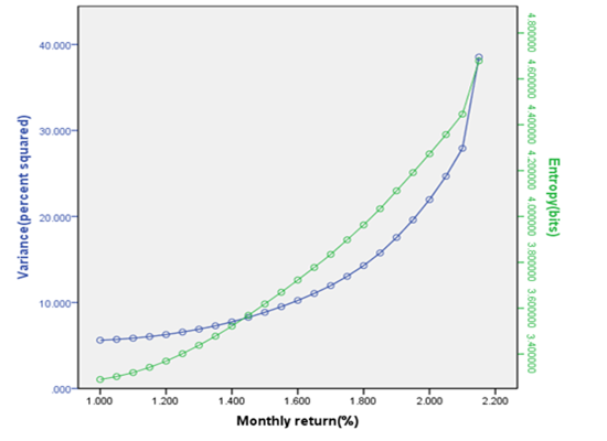
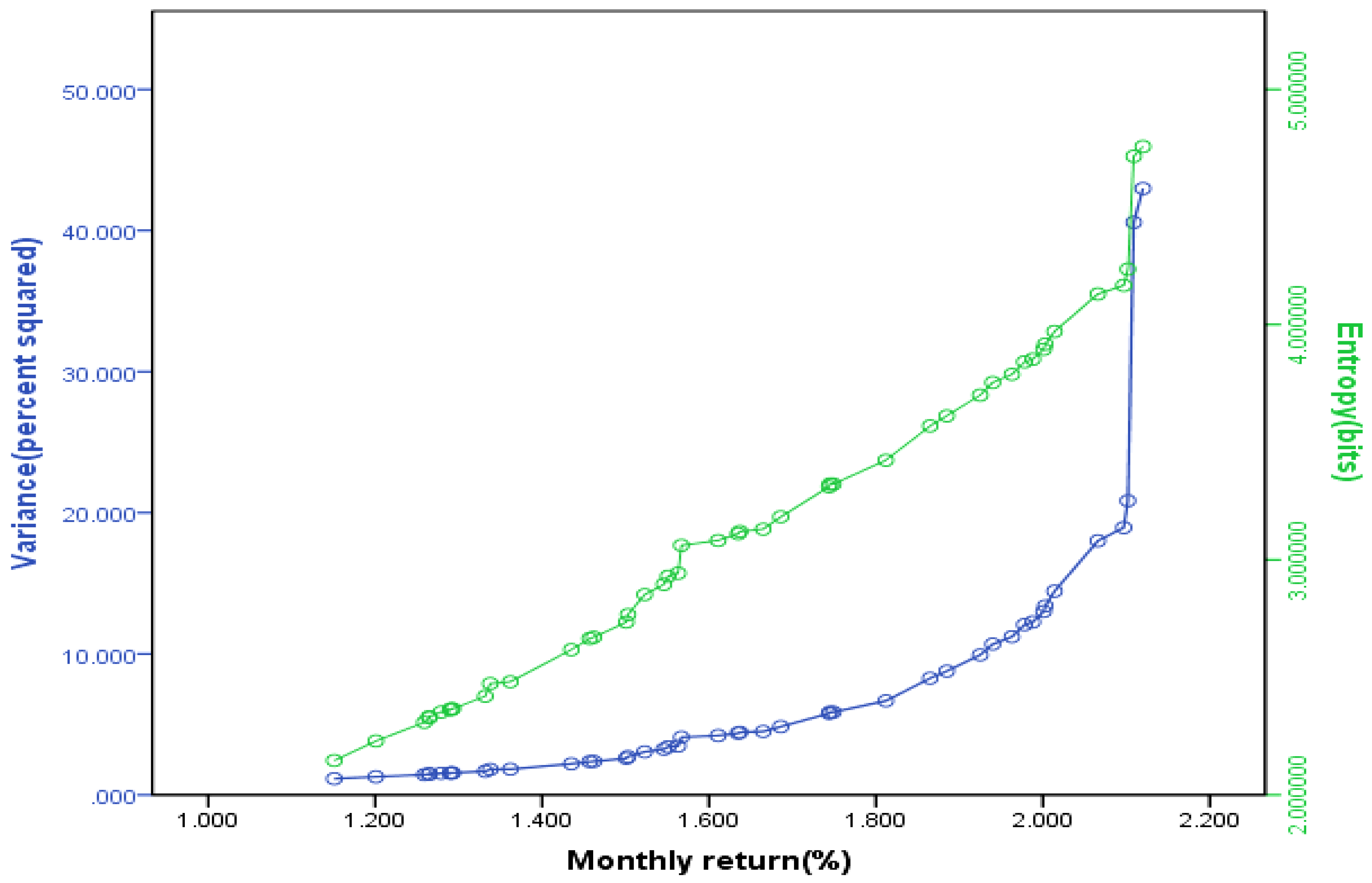
where Rit = return on security i in period t; Pit = price of security i in period t; Dit = cash dividend for security i in period t. The securities in the sample belong to the following industries according to Standard Industrial Classification: (1) Health and Personal Care; (2) Leisure Time and Services; (3) Technology; (4) Consumer Goods; (5) Basic Industries; (6) Utilities; (7) Finance; and (8) Oil. The Markowitz full-covariance efficient frontier and its corresponding mean-entropy frontier for 24 corner portfolios were computed as shown in Figure 1. And the Sharpe single-index efficient frontier and its corresponding index-based mean-entropy frontier for 47 corner portfolios were also computed, as shown in Figure 2.
We can see the mean-entropy portfolios are consistent with the Markowitz full covariance and the Sharpe single-index models. The observed differences between the frontiers in each case are due primarily to the scales employed in the graphs.
When replying the comments raised by White [51], Philippatos and Wilson reiterated that the mean-entropy model was not intended to be used for distributions that have not been modeled in portfolio selection, including some single-parameter discrete distributions such as Bernoulli, Possion, and Geometric distributions, and some continuous distributions such as the exponential distributions [52]. They argued that although entropy provides an ideal means of relating earnings reports and insiders’ activities to the distributions of returns, it is not always applicable since information (entropy) is additive no matter what the source is. The decision to use uncertainty (entropy) analysis depends not only on the properties of the criterion variables but also on the expected benefits from being more sensitive rather than more general.
Figure 1.
The Markowitz full-covariance efficient frontier and its corresponding mean-entropy frontier for 24 corner portfolios.
Figure 1.
The Markowitz full-covariance efficient frontier and its corresponding mean-entropy frontier for 24 corner portfolios.

Figure 2.
The Sharpe single-index efficient frontier and its corresponding index-based mean-entropy frontier for 47 corner portfolios.
Figure 2.
The Sharpe single-index efficient frontier and its corresponding index-based mean-entropy frontier for 47 corner portfolios.

In fuzzy portfolio selection theories, entropy can also be used as the measure of risk. The smaller the entropy value is, the less uncertainty the portfolio return contains, and thus, the safer the portfolio is. Huang compared the fuzzy mean-variance model with the fuzzy mean-entropy model in two special cases and presented a hybrid intelligent algorithm to solve the proposed models in general cases [13]. He argued that a conservative investor requires the portfolio to be relatively safe before pursue maximum expected return, which can be expressed in the mean-entropy model as follows:
subject to:
On the other hand, if the investor is bold, he or she will require the expected return to be high enough before minimizing the risk level, as expressed in the following way:
subject to:
where is the investment proportion in securities i, and ξi are fuzzy variables and represent the returns of the ith securities, which is defined as i = 1,2,…,n, respectively, where is the estimated closing prices of the securities i in the future, yi is the closing prices of the securities i at present, and di is the estimated dividends of the securities i from now to the future time. γ is the maximum entropy level the investors can tolerate, so it is reasonable to ask that the entropy value of the portfolio must first be lower than or equal to a safety level; α is the lowest return level the investor feels is satisfactory. And H denotes the entropy of the fuzzy variables and E is the expected value operator.
Huang compared the fuzzy mean-variance model with the fuzzy mean-entropy model and proved that when fuzzy security returns are all normally distributed or symmetric triangular, the optimal solution of model (28) is the same as that of the fuzzy mean-variance model. The fuzzy mean-variance model given in Reference [25] was:
subject to:
where V is the variance operator and vice versa. In other cases of fuzzy security returns, Huang employed a fuzzy simulation integrated genetic algorithm to solve the proposed model.
4.2. Entropy as a Measure of Capital Increment
When Markowitz’s method was applied to the portfolio selection, the speed of capital increment was ignored. In 2005, the incremental entropy (H in Equation (13)), which measured the time needed for capital to double, was created by Ou [6]. The incremental entropy formula has no negative symbol as does generalized entropy formula. It is similar to the formula of average coding length in information theory. Instead of expectations and standard deviations of returns as in Markowitz’s theory, the theory of incremental entropy employs the extent and possibility of gain and loss to describe investment value. Using Lagrange multiplier, Ou drew a conclusion that when gain and loss were equally possible, if the possible loss was up to 100 percent, one should not invest more than 50 percent of total fund no matter how high the possible gain might be. This conclusion is meaningful for high risk investments, such as futures, options, etc. etc. Many new investors in future markets lose their money very fast because their investment ratios are not controlled well and generally too high.
4.3. Entropy as a Measure of Portfolio Diversification
Entropy is a widely accepted measure of diversity [53,54,55,56,57,58,59,60]. It is well known that the greater the level of entropy, the higher the degree of portfolio diversification. Early literature using entropy as an objective function in multi-objective model of portfolio selections include Bera and Park [56], Usta and Kantar [57], Jana, Roy and Mazumder [9,58], Samanta and Roy [59], etc. Bera and Park [56,60] presented asset allocation models based on entropy and cross entropy measures in order to generate a well-diversified portfolio. If entropy is used as an objective function to determine portfolio weights, the obtained weights become automatically non-negative. This means that a model with entropy yields no short-selling, and due to theoretical and practical reasons, the portfolio with no short-selling is preferred by conservative investors [9].
A multi-objective approach based on a mean-variance-skewness-entropy portfolio selection model (MVSEM) has been investigated by many scholars in finance. This approach adds an entropy measure to the mean-variance-skewness model (MVSM) to generate a well-diversified portfolio. Usta and Kantar employed the Shannon’s entropy measure H(x) in Equation (2) as the measure of portfolio diversification [7]. A well-diversified optimal portfolio problem could be solved as:
subject to where xi is the proportion invested in risky asset i, j = 1,2,…,n; xn+1 is the proportion invested in the riskless asset; Ri is the random rate of return on the risky asset i, i = 1,2,…,n; rn+1 is the rate of return on riskless asset; ri is E(Ri), the expected rate of return on the risky asset i, i = 1,2,…,n; σij is Cov(Ri,Rj), the covariance between Ri and Rj, i, j = 1,2,…,n; Υijk is E[(Ri−ri)(Rj−rj)(Rk−rk)], central third moment of returns, i, j, k = 1,2, …,n. And the return of a portfolio x = (x1,x2,…, xn) is:
Usta and Kantar’s empirical study was based on three datasets. The first dataset consisted of monthly returns on 20 industry portfolios in the United States. The second dataset consisted of monthly returns of seven international equity indexes for G-7 countries. The last dataset includes monthly returns of 15 assets traded on the Istanbul Stock Exchange in Turkey. They evaluated the out-of-sample performance of MVSEM relative to well-known portfolio models such as the equally weighted model (EWM), minimum variance model (MinVM), MVM and MVSM. The performance of the MVSEM was assessed in terms of the following measures: Sharpe ratio (SR), adjusted Sharpe ratio for skewness (ASR), mean absolute deviation ratio (MADR), Sortino-Satchell ratio (SSR), Farinelli-Tibiletti ratio (FTR), generalized Rachev ratio (GRR) and portfolio turnover (PT). They also computed Jobson and Korkie’s ZJK test statistics to evaluate the statistical significance for the difference in Sharpe ratios among the considered models in this study. For the first dataset, the MVSEMs provided best results in terms of all performance measures except GRRs, which favored the EWMs. For the second dataset, the MVSEMs performed better than MVM, MinVM and MVSM according to all considered performance measures except GRR, and the values of PT of all MVSEMs were smaller than the MVM, MinVM and MVSM. For the third dataset, the MVSEMs outperformed the other models in terms of most of the performance measures, and the values of PT for the MVSEMs were substantially less than that for the others. So they confirmed the significant effect of MVSEMs and the significant effect of entropy in portfolio selection models.
Same as the multi-period portfolio selection problem, entropy can also be used in other models as the degree of portfolio diversification. In 2012, some Chinese scholars tried to solve the decentralized investment problem for multi-period fuzzy portfolio selection [10]. They presented a possibilistic mean-semivariance-entropy model with four criteria: return, risk, transaction cost and degree of portfolio diversification. They designed the novel possibilistic entropy which overcame the shortcomings of the proportion entropy models in Jana et al. [9] and Kapur [61]. The mathematical expression of the multi-period entropy can be expressed as follows:
where represents the reward-to-variability ratio of asset i at period t; is the adjustment coefficient of xt,i ; ε is a sufficiently small positive number; rf(t) is the risk-free return rate of the portfolio at period t; E(rt,i) and Var(rt,i) denote the possibilistic mean and variance of the fuzzy return rate on asset i at period t, respectively. They used datasets from Shanghai Stock Exchange to create two examples to test the effectiveness of the proposed approach and the feasibility of the designed algorithm. The results comparing the two examples showed that the designed possibilistic entropy could be an effective notation for distributive investment.
5. Applications of Entropy in Asset Pricing
As pointed out in Section 1, the concepts of entropy and its relevant principles are also used considerably in the field of asset pricing.
5.1. Entropy in Option Pricing
Back in 1996, Buchen and Kelly tackled the general problem of how to extract an asset probability distribution from limited and incomplete market information available on an options exchange. The implementations of the MEP in the cases of simple call and put options were showed as below. They assumed that the underlying asset pays no dividends, and they set up usual assumptions for European options in an equilibrium market, where the usual assumptions including no transaction expenses and no taxes, no arbitrage opportunities. The Maximum Entropy Distribution (MED) is given in Equation (34) with constraint functions ci(x):
where the is the Lagrange multiplier.
Let i index the strike prices Ki, then for a call option:
and for a put option:
The function D(T) denotes the non-stochastic present-value discount factor to time T and acts only as a multiplicative constant. For example, we can choose with a constant risk-free rate r or some other suitable representation such as the price of a bond with face value $1 and maturing at time T.
They developed an expectation pricing model and a set of option prices at different strikes. Those data were insufficient to determine the distribution of the underlying asset. However, if these prices were used to constrain the distribution that otherwise had maximum entropy (or minimum cross-entropy), a unique distribution was obtained. Their research showed that the maximum entropy distribution was able to fit a known density accurately, given simulated option prices at different strikes [18].
Buchen and Kelly’s method has important meanings and attracted some authors to continue their research and compare it with other methods. One criticism often raised is that the method of finding the form of the density using Lagrange multipliers is not rigorous. Instead of the Lagrange multiplier method, Neri and Schneider [19] set up a simple and robust algorithm for the maximum entropy distribution. This algorithm worked well in practice and led to the correct form, and they also gave a complete mathematical proof. Their proof used results of Csiszár [62] that gave additional insights into “distances” between distributions and establish remarkable “geometric” results.
In the field of option pricing, Gulko [15] has to be mentioned here. He formulated the maximum-entropy framework by introducing the EPT in 1997. In his opinion, the EPT offers the construction of unique risk-neutral probabilities in both complete and incomplete market economies. The EPT suggests that, in information efficient markets, plausible market beliefs are not equally likely and that the maximum-entropy or maximum missing information must prevail. He also applied the EPT to the canonical option valuation problems—stock option pricing [16] and bond option pricing [17]. He claimed that the maximum-entropy density p(r) is a joint normal density in the return space which is a dart board and repeat the dart-board argument on R. He showed that a joint normal density solves the following program:
subject to , u(r) > 0 on R.
The maximum is a probability density of the form , where is the Lagrange multiplier associated with the moment constraint vij, r = [ri] is the column vector of random stock returns, where ri is a random return on asset i for 1 ≤ i ≤ n, p(r) is the maximum-entropy joint probability density of stock returns, and μ = [μi] ≡ E(r) with μi ≡ E(ri) for 1 ≤ i ≤ n, V = [vj] is a known covariance matrix of the returns with vij = E[(ri−μi)(rj−μj)] for 1 ≤ i, j ≤ n. Assume the return on any stock cannot be expressed as a linear combination of the returns on other stocks, so the covariance matrix V is nonsingular. Therefore, in a stock market, the maximum-entropy density p(r) is a joint normal as follows:
where |V| denotes the determinant of V. Also, by analogy with the univariate case, the joint density f(ST) of the random stock prices is a multivariate lognormal.
With current stock price S, current riskless bond price P and strike price K, the gamma density is:
Where .
Then the cumulative gamma distribution function can be denoted by:
and the complementary cumulative gamma function can be denoted by:
Therefore, the gamma prices of European call and put options on dividend protected stocks are respectively as following:
The gamma formulae above require only four “observable” inputs: K, P, S, and σ2. These formulae have the structure and simplicity of the Black-Scholes stock option model. They also feature many Black-Scholes-like properties. However, unlike the Black-Scholes model, the gamma model imposes no restrictions on the dynamics of the stock price or stock returns. Instead, the gamma model parameterizes the price dynamics of an imaginary constant-cash-flow security. The price process S(t) for the actual stock is immune to this parameterization. For example, the parameterization of x(t) does not prevent the volatility of the actual stock price from being random. Also, unlike the Black-Scholes model, the gamma formula is valid for arbitrary dynamics of short-term interest rates.
Similar to the stock option pricing, Gulko applied the EPT to the famous Vasicek-Jamshidian model (the model specifies that the instantaneous interest rate follows the stochastic differential equation:
where Wt is a Wiener process under the risk neutral framework modeling the random market risk factor, in that it models the continuous inflow of randomness into the system. The standard deviation parameter, σ, determines the volatility of the interest rate and in a way characterizes the amplitude of the instantaneous randomness inflow. The typical parameters b, a and σ, together with the initial condition r0 , completely characterize the dynamics, and can be quickly characterized as follows, assuming a to be non-negative) [59] and made some useful improvements [17]. Gulko’s new model was different from Vasicek-Jamshidian model in the following ways that show its advantages. First, unlike the Vasicek-Jamshidian model, the Call formula did not restrict movements of term structure of interest rates. Second, the Vasicek-Jamshidian model was valid only in a complete market, while the Call formula was valid in both complete and incomplete markets. Third, the Vasicek-Jamshidian model was suitable for pricing options on default-free bonds only, while the Call formula (43) was suitable for pricing options on both default-free and risky bonds.
However, Gulko’s method can only solve the problem of European bond option pricing. American bond options are generally believed difficult to price since the process requires numerical methods. In order to apply the entropy method to American bond option pricing, Zhou et al. formulated a new entropy model on the basis of Gulko’s entropy pricing theory as well as Geske-Johnson’s method of analytical approximation of American options [63]. In another thesis Zhou et al. [64] believed that the option pricing in incomplete markets should differ from that in complete markets. Therefore the classical Black-Scholes option pricing model may be unsuitable in incomplete markets. They developed an analytical formula to value caps, floors, collars and swaptions of interest rates with parallel to Black-Scholes option pricing model on the basis of the entropy pricing method. Zhou and Wang [65] extended the research to the hedging parameters in incomplete markets. They followed the Black-Scholes model to define and formulate a series of hedging parameters, and performed numerical simulations based on the entropy model. They compared the results with those obtained under the framework of the Black-Scholes model. Their results showed that the sensitivity degrees of the entropy model were larger than those of the Black-Scholes model and therefore proved the entropy model is a new and better method for the risk management of derivatives in an incomplete market.
Recently, Trivellato illustrated some financial applications of the Tsallis and Kaniadakis deformed exponentials [66,67]. The Kaniadakis exponential [68] was introduced to define a new family of martingale measures based on the standard entropy martingale measure [27] and the well-known p-martingale measures [30]. It has proven to be suitable to explain a very large class of experimentally observed phenomena [69,70,71]. The φ-logarithm was used to introduce the notion of φ-divergence between two probability measures, which extends the standard Kullback-Leibler divergence. The minimization of this deformed divergence was proposed as a general criterion to select a pricing measure in incomplete markets. He investigated the relationships between this relative entropy and the deformed Tsallis and Kaniadakis relative entropies, and illustrated their applications in finance, especially generalizing the well-known Black-Scholes model. The Kaniadakis entropy can be described as follows:
where .
5.2. Entropy in Other Derivative Securities Pricing
Derivative securities are financial contracts valued as functions of the future values of the underlying asset(s). Examples of derivative securities include, but are not limited to, futures, options, swaps, interest-rate caps and floors, warrants, and convertible bonds. To utilize derivative securities successfully one must be able to price them and to calculate their price changes following price changes in the underlying asset(s). To calculate price one needs: (i) the points in time where the derivative security generates cash flows, (ii) the cash flow generated by the derivative security as a function of the level of the underlying asset(s) at the points in time specified in (i), (iii) the discount factors associated with these points in time, and (iv) the probability of underlying asset(s)’s value being at certain levels at the points in time specified in (i). Given items (i)–(iv) one simply multiplies all cash flows by the appropriate probability and discount factor and sums them up [25]. Accurate pricing hinges ultimately on item (iv).
Other derivative securities than options can also be priced by the method we introduce in Section 2 and Section 3. For example, Branger [31] proposed two methods to determine the pricing function for derivatives when the market was incomplete. He chose an equivalent martingale measure with minimal cross-entropy relative to a given benchmark measure. His research showed that the choice of the numeraire had an impact on the resulting pricing function, but there was no sound economic answer to the question of which numeraire to choose. The ad-hoc choice of numeraire introduced an element of arbitrariness into the pricing function which contradicts the motivation to be the least prejudiced way to choose the pricing operator. His two new methods to select a pricing function were: the stochastic discount factor (SDF) with minimal extended cross-entropy relative to a given benchmark SDF, and the Arrow-Debreu (AD) prices with minimal extended cross-entropy relative to some set of benchmark AD prices. His research showed that these two methods are equivalent in that they generate identical pricing functions. They avoided depending on the numeraire by replacing it with the benchmark pricing function which can be chosen based on economic conditions rather than arbitrarily.
6. Applications of Entropy in Other Fields of Finance
Besides the portfolio selection and asset pricing we introduced above, the entropy has been used in many other fields of finance.
The two Canadian authors Choulli and Hurd extended the Hellinger process (for 0 < q < 1 and L a local martingale such that 1+∆L > 0 P-almost surely, the following assertions hold:
- (1)
- The process ε(L)q is a supermartingale;
- (2)
- There exists a predictable increasing process h(q) such that h0(q) = 0 andis a martingale.
When this theorem 4.1 is applied to a martingale Z for a pair Q < P, the resulting process h(q)(P,Q) is called a q-Hellinger process) to entropy distance and f-divergence distances [72]. In 2008, Hackworth used entropy to propose a logistic model so as to combine uncertainty with the yield curve, or interest rate term structure [73]. His model produced yield curves virtually identical to those of the Bank of England except at the short end where the Bank used zero coupon bonds data. In order to distinguish the risk of treasury bonds with same structure, property and duration but different price, Zhou and Xiong [74] proposed to use the information entropy to measure the risk. Their empirical study based on Chinese stock market had consistent results with the convexity, variance and VaR methods.
Entropy also plays an important role in utility functions which represent the degree of satisfaction of investors. Candeal et al. [75] found a striking similarity between the utility functions in economics and the entropy in thermodynamics. Abbas et al. [76] developed an optimal algorithm to obtain Von Neumann-Morgenstern utility value choice. Abbas [77] introduced the concept of density function of utility and proposed a new method to determine the utility value on the basis of MEP and preference behavior. Yang et al. [78] proposed the risk measure of expected utility-entropy and established a relevant model. Zhou et al. [79] reviewed the applications of entropy in utility and decision fields, and discussed future developments in these fields.
In recent years, some scholars have concentrated on the applications of MEP in other fields of finance. Li [80] priced longevity risk by a pricing method which was based on the maximization of the Shannon entropy, and he implemented this method with the parametric bootstrap. Mistrulli [81] analyzed how contagion propagates within the Italian interbank market using a unique data set, his results obtained by assuming the maximum entropy were compared with those reflecting the observed structure of interbank claims. In addition, Ortiz-Cruz et al. [82] analyzed the evolution of the informational complexity and efficiency for the crude oil market with entropy methods.
Obviously, the development of the applications of entropy can be seen of great importance. We can look forward to deeper research of entropy in other fields of finance.
7. Conclusions
Although the word entropy was originally used in thermodynamics, its concepts and relevant principles have been applied to the field of finance for a long period of time. Entropy has its unique advantages in measuring risk and describing distributions. As a result, the applications of entropy in finance are important. This paper reviews representative work regarding the applications of entropy in finance, mainly in portfolio selection and asset pricing.
In the field of portfolio selection, entropy was first used as a measure of risk. Some scholars replaced variance with entropy in typical mean-variance models. Some others added entropy to original portfolio models and optimized the new models. Entropy has also been applied in the fuzzy portfolio selection situation as a measure of risk. Moreover entropy can act as a measure of portfolio diversification and capital increment. Scholars found that the empirical results of portfolio selection models with entropy were consistent with those of the original models. Although these research results were queried by others, the contributions they made to the portfolio selection cannot be ignored.
The concepts and principles of entropy can be used more widely in asset pricing. It helps scholars tackle the general problem of extracting asset probability distributions from limited and incomplete market information. It is also helpful in solving the canonical option valuation problems. The entropy pricing theory and the principle of maximum entropy were used most frequently in setting up different pricing models and developing corresponding algorithms.
However, current studies on entropy are still at a preliminary stage. Problems that haven’t been dealt with include the extreme conditions of forms and principles of entropy. There is plenty of work to do to improve the entropy theory. We will continue to pay attention to the progress in this field.
Acknowledgments
The authors would like to thank the editor and three anonymous referees for their valuable comments and suggestions. This work is partially supported by grants from the National Natural Science Foundation of China (No.71171012, 71371024), Chinese Universities Scientific Fund of Beijing University of Chemical Technology (No.ZZ1319, ZZ1320), and The National Science and Technology Support Program (No.2013BAK04B02).
Conflicts of Interest
The authors declare no conflict of interest.
References
- Laidler, K.J. Thermodynamics. In The World of Physical Chemistry; Oxford University Press: New York, NY, USA, 1995; pp. 156–240. [Google Scholar]
- Clausius, R. Ueber verschiedene für die Anwendung bequeme formen der Hauptgleichungen der mechanischen Wärmetheorie. Ann. Phys. Chem. 1865, 125, 53–400. [Google Scholar] [CrossRef]
- Liu, Y.; Liu, C.J.; Wang, D.H. Understanding atmospheric behaviour in terms of entropy: a review of applications of the second law of thermodynamics to meteorology. Entropy 2011, 13, 211–240. [Google Scholar] [CrossRef]
- Brissaud, J.B. The meanings of entropy. Entropy 2005, 7, 68–96. [Google Scholar] [CrossRef]
- Philippatos, G.C.; Wilson, C.J. Entropy, market risk, and the selection of efficient portfolios. Appl. Econ. 1972, 4, 209–220. [Google Scholar] [CrossRef]
- Ou, J.S. Theory of portfolio and risk based on incremental entropy. J. Risk Finance 2005, 6, 31–39. [Google Scholar] [CrossRef]
- Xu, J.P.; Zhou, X.Y.; Wu, D.D. Portfolio selection using λ mean and hybrid entropy. Ann. Oper. Res. 2011, 185, 213–229. [Google Scholar] [CrossRef]
- Usta, I.; Kantar, Y.M. Mean-variance-skewness-entropy measures: a multi-objective approach for portfolio selection. Entropy 2011, 13, 117–133. [Google Scholar] [CrossRef]
- Jana, P.; Roy, T.K.; Mazumder, S.K. Multi-objective possibilistic model for portfolio selection with transaction cost. J. Comput. Appl. Math. 2009, 228, 188–196. [Google Scholar] [CrossRef]
- Zhang, W.G.; Liu, Y.J.; Xu, W.J. A possibilistic mean-semivariance-entropy model for multi-period portfolio selection with transaction costs. Eur. J. Oper. Res. 2012, 222, 341–349. [Google Scholar] [CrossRef]
- Zhou, R.X.; Wang, X.G.; Dong, X.F.; Zong, Z. Portfolio selection model with the measures of information entropy-incremental entropy-skewness. Adv. Inf. Sci. Service Sci. 2013, 5, 853–864. [Google Scholar]
- Smimoua, K.; Bector, C.R.; Jacoby, G. A subjective assessment of approximate probabilities with a portfolio application. Res. Int. Bus. Finance 2007, 21, 134–160. [Google Scholar] [CrossRef]
- Huang, X.X. Mean-entropy models for fuzzy portfolio selection. IEEE Tran. Fuzzy Syst. 2008, 16, 1096–1101. [Google Scholar] [CrossRef]
- Rödder, W.; Gartner, I.R.; Rudolph, S. An entropy-driven expert system shell applied to portfolio selection. Expert Syst. Appl. 2010, 37, 7509–7520. [Google Scholar] [CrossRef]
- Gulko, L. Dart boards and asset prices introducing the entropy pricing theory. Adv. Econom. 1997, 12, 237–276. [Google Scholar]
- Gulko, L. The entropy theory of stock option pricing. Int. J. Theoretical Appl. Finance 1999, 2, 331–355. [Google Scholar] [CrossRef]
- Gulko, L. The entropy theory of bond option pricing. Int. J. Theoretical Appl. Finance 2002, 5, 355–383. [Google Scholar] [CrossRef]
- Buchen, P.W.; Kelly, M. The maximum entropy distribution of an asset inferred from option prices. J. Financ. Quant. Anal. 1996, 31, 143–159. [Google Scholar] [CrossRef]
- Neri, C.; Schneider, L. Maximum entropy distributions inferred from option portfolios on an asset. Finance Stochast. 2012, 16, 293–318. [Google Scholar] [CrossRef]
- Krishnan, H.; Nelken, L. Estimating implied correlations for currency basket options using the maximum entropy method. Derivatives Use Trading Regul. 2001, 7, 1–7. [Google Scholar]
- Rompolis, L.S. Retrieving risk neutral densities from European option prices based on the principle of maximum entropy. J. Empir. Finance 2010, 17, 918–937. [Google Scholar] [CrossRef]
- Guo, W.Y. Maximum entropy in option pricing: a convex-spline smoothing method. J. Futures Markets 2001, 21, 819–832. [Google Scholar] [CrossRef]
- Borwein, J.; Choksi, R.; Maréchal, P. Probability distributions of assets inferred from option prices via the principle of maximum entropy. J. Soc. Ind. Appl. Math. 2003, 14, 464–478. [Google Scholar] [CrossRef]
- Stutzer, M. A simple nonparametric approach to derivative security valuation. J. Finance 1996, 51, 1633–1652. [Google Scholar] [CrossRef]
- Hawkins, R.J. Maximum entropy and derivative securities. Adv. Econometrics 1997, 12, 277–300. [Google Scholar]
- Kullback, S.; Leibler, R.A. On information and sufficiency. Ann. Math. Stat. 1951, 22, 79–86. [Google Scholar] [CrossRef]
- Frittelli, M. The minimal entropy martingale measure and the valuation problem in incomplete markets. Math. Finance 2000, 10, 39–52. [Google Scholar] [CrossRef]
- Benth, F.E.; Groth, M. The minimal entropy martingale measure and numerical option pricing for the Barndorff-Nielsen-Shephard stochastic volatility model. Stoch. Anal. Appl. 2009, 27, 875–896. [Google Scholar] [CrossRef]
- Hunt, J.; Devolder, P. Semi-Markov regime switching interest rate models and minimal entropy measure. Phys. A 2011, 390, 3767–3781. [Google Scholar] [CrossRef]
- Grandits, P. The p-optimal martingale measure and its asymptotic relation with the minimal entropy martingale measure. Bernoulli 1999, 5, 225–247. [Google Scholar] [CrossRef]
- Branger, N. Pricing derivative securities using cross-entropy an economic analysis. Int. J. Theor. Appl. Finance 2004, 7, 63–81. [Google Scholar] [CrossRef]
- Shannon, C.E. A mathematical theory of communication. Bell Syst. Tech. J. 1948, 27, 379–423. [Google Scholar] [CrossRef]
- Tsallis, C. Possible generalization of Boltzmann-Gibbs statistics. J. Stat. Phys. 1988, 52, 479–487. [Google Scholar] [CrossRef]
- Havrda, J.; Charvát, F. Quantification method of classification processes: concept of structural α-entropy. Kybernetika 1967, 3, 30–35. [Google Scholar]
- Patil, G.P.; Taillie, C. Diversity as a concept and its measurement. J. Am. Stat. Assoc. 1982, 77, 548–561. [Google Scholar] [CrossRef]
- Tsallis, C. Generalized entropy-based criterion for consistent testing. Phys. Rev. E 1998, 58, 1442–1445. [Google Scholar] [CrossRef]
- Luca, A.D.; Termini, S. A definition of non-probabilistic entropy in the setting of fuzzy sets theory. Inf. Control 1972, 20, 301–312. [Google Scholar] [CrossRef]
- Bhandari, D.; Pal, N.R. Some new information measures for fuzzy sets. Inf. Sci. 1993, 67, 209–228. [Google Scholar] [CrossRef]
- Kosko, B. Fuzzy entropy and conditioning. Inf. Sci. 1986, 40, 165–174. [Google Scholar] [CrossRef]
- Pal, N.R.; Bezdek, J.C. Measuring fuzzy uncertainty. IEEE Trans. Fuzzy Syst. 1994, 2, 107–118. [Google Scholar] [CrossRef]
- Yager, R.R. On the entropy of fuzzy measures. IEEE Trans. Fuzzy Syst. 2000, 8, 453–461. [Google Scholar] [CrossRef]
- Li, X.; Liu, B. Maximum entropy principle for fuzzy variable. Int. J. Uncertain. Fuzz. 2007, 15, 43–52. [Google Scholar] [CrossRef]
- Li, P.; Liu, B. Entropy and credibility distributions for fuzzy variables. IEEE Trans. Fuzzy Syst. 2008, 16, 123–129. [Google Scholar]
- Brody, D.C.; Buckley, I.R.C.; Constantinou, I.C. Option price calibration from Rényi entropy. Phys. Lett. 2007, 366, 298–307. [Google Scholar] [CrossRef]
- Liese, F.; Vajda, I. On divergences and informations in statistics and information theory. IEEE Trans. Inform. Theor. 2006, 52, 4394–4412. [Google Scholar] [CrossRef]
- Balestrino, A.; Caiti, A.; Crisostomi, E. Generalised entropy of curves for the analysis and classification of dynamical systems. Entropy 2009, 11, 249–270. [Google Scholar] [CrossRef]
- Csiszár, I. Eine Informationstheoretische Ungleichung und ihre Anwendung auf den Beweis der Ergodizität on Markoffschen Ketten. Publ. Math. Inst. Hungar. Acad. Sci. 1963, 8, 84–108. [Google Scholar]
- Ali, M.S.; Silvey, D. A general class of coefficients of divergence of one distribution from another. J. Roy. Stat. Soc. B 1966, 28, 131–140. [Google Scholar]
- Kapur, J.N.; Kesavan, H.K. Jaynes’ Maximum Entropy Principle. In Entropy Optimization Principles with Applications; Academic Press: San Diego, CA, USA, 1992; pp. 23–151. [Google Scholar]
- Markowitz, H. Portfolio selection. J. Finance 1952, 7, 77–91. [Google Scholar]
- White, D.J. Entropy, market risk and the selection of efficient portfolios: comment. Appl. Econ. 1974, 6, 73–75. [Google Scholar] [CrossRef]
- Philippatos, G.C.; Wilson, C.J. Entropy, market risk and the selection of efficient portfolios: reply. Appl. Econ. 1974, 6, 77–81. [Google Scholar] [CrossRef]
- Hoskisson, R.E.; Hitt, M.A.; Johnson, R.H.; Moesel, D. Construct validity of an objective (entropy) categorical measure of diversification strategy. Strat. Manag. J. 2006, 14, 215–235. [Google Scholar] [CrossRef]
- Dionísio, A.; Menezes, R.; Mendes, D.A. Uncertainty Analysis in Financial Markets: Can Entropy be a Solution? In Proceedings of the 10th Annual Workshop on Economic Heterogeneous Interacting Agents, University of Essex, Colchester, UK, 13 June 2005.
- Philippatos, G.C.; Gressis, N. Conditions of equivalence among E-V, SSD and E-H portfolio selection criteria: The case for uniform, normal and lognormal distributions. Manag. Sci. 1975, 21, 617–625. [Google Scholar] [CrossRef]
- Bera, A.K.; Park, S.Y. Optimal Portfolio Diversification Using the Maximum Entropy Principle. In Proceedings of the Second Conference on Recent Developments in the Theory, Method, and Applications of Information and Entropy Econometrics, Washington DC, WA, USA, 23 September 2009.
- Usta, I.; Kantar, Y.M. Analysis of Multi-objective Portfolio Models for the Istanbul Stock Exchange. In Proceedings of the 2nd International Workshop on Computational and Financial Econometrics, Neuchatel, Switzerland, 19 June 2008.
- Jana, P.; Roy, T.K.; Mazumder, S.K. Multi-objective mean-variance-skewness model for portfolio optimization. Appl. Math. Optim. 2007, 9, 181–193. [Google Scholar]
- Samanta, B.; Roy, T.K. Multi-objective portfolio optimization model. Tamsui Oxf. J. Math. Sci. 2005, 21, 55–70. [Google Scholar]
- Bera, A.K.; Park, S.Y. Optimal portfolio diversification using the maximum entropy principle. Economet. Rev. 2008, 27, 484–512. [Google Scholar] [CrossRef]
- Kapur, J.N. Maximum-Entropy Probability Distributions: Principles, Formalism and Techniques. In Maximum Entropy models in Science and Engineering; Wiley Eastern Limited: New Delhi, India, 1990; pp. 1–146. [Google Scholar]
- Csiszár, I. I-divergence geometry of probability distributions and minimization problems. Ann. Probab. 1975, 3, 146–158. [Google Scholar] [CrossRef]
- Zhou, R.X.; Chen, L.M.; Qiu, W.H. The entropy model of American bond option pricing. Math. Pract. Theor. 2006, 36, 59–64. [Google Scholar]
- Zhou, R.X.; Sun, J.; Xu, J.R. Valuation of interest rate options based on the entropy pricing method under incomplete market. J. Beijing Univ. C.T. 2008, 35, 101–103. [Google Scholar]
- Zhou, R.X.; Wang, X.G. Study of hedging parameters based on the entropy model of stock option pricing. J. Beijing Univ. C. T. 2009, 36, 100–104. [Google Scholar]
- Trivellato, B. The minimal k-entropy martingale measure. Int. J. Theor. Appl. Finance 2012, 15, 1–22. [Google Scholar] [CrossRef]
- Trivellato, B. Deformed exponentials and applications to finance. Entropy 2013, 15, 3471–3489. [Google Scholar] [CrossRef]
- Kaniadakis, G. Non-linear kinetics underlying generalized statistics. Phys. A 2001, 296, 405–425. [Google Scholar] [CrossRef]
- Kaniadakis, G. H-theorem and generalized entropies within the framework of nonlinear kinetics. Phys. Lett. A 2001, 288, 283–291. [Google Scholar] [CrossRef]
- Kaniadakis, G. Statistical mechanics in the context of special relativity. Phys. Rev. E 2002, 66, 056125. [Google Scholar] [CrossRef]
- Kaniadakis, G.; Scarfone, A.M. Lesche stability of kappa-entropy. Phys. Stat. Mech. Appl. 2004, 340, 102–109. [Google Scholar] [CrossRef]
- Choulli, T.; Hurd, T.R. The role of Hellinger Processes in mathematical finance. Entropy 2001, 3, 150–161. [Google Scholar] [CrossRef]
- Hackworth, J.F. Uncertainty and the yield curve. Econ. Lett. 2008, 98, 259–268. [Google Scholar] [CrossRef]
- Zhou, R.X.; Xiong, M.H. Treasury Risk Measurement and Empirical Comparison-based on Information Entropy. In Proceedings of World Automation Congress, Puerto Vallarta, Jalisco, Mexico, 24 June 2012.
- Candeal, J.C.; De Miguel, J.R.; Indur, A.E. Utility and entropy. Econ. Theor. 2001, 17, 233–238. [Google Scholar] [CrossRef]
- Abbas, A.E. Entropy methods for adaptive utility elicitation. IEEE Trans on Systems 2004, 34, 169–178. [Google Scholar] [CrossRef]
- Abbas, A.E. Maximum entropy utility. Oper. Res. 2006, 54, 277–290. [Google Scholar] [CrossRef]
- Yang, J.P.; Qiu, W.H. A measure of risk and a decision making model based on expected utility and entropy. Eur. J. Oper. Res. 2005, 164, 792–799. [Google Scholar] [CrossRef]
- Zhou, R.X.; Liu, S.C.; Qiu, W.H. Survey of applications of entropy in decision analysis. Control Decis. 2008, 23, 361–371. [Google Scholar]
- Li, J.S. Pricing longevity risk with the parametric bootstrap: A maximum entropy approach. Insur. Math. Econ. 2010, 47, 176–186. [Google Scholar] [CrossRef]
- Mistrulli, P.E. Assessing financial contagion in the interbank market: Maximum entropy versus observed interbank lending patterns. J. Bank. Finance 2011, 35, 1114–1127. [Google Scholar] [CrossRef]
- Ortiz-Cruz, A.; Rodriguez, E.; Ibarra-Valdez, C.; Alvarez-Ramirez, J. Efficiency of crude oil markets: Evidences from informational entropy analysis. Energ. Pol. 2012, 41, 365–373. [Google Scholar] [CrossRef]
© 2013 by the authors; licensee MDPI, Basel, Switzerland. This article is an open access article distributed under the terms and conditions of the Creative Commons Attribution license (http://creativecommons.org/licenses/by/3.0/).
Share and Cite
MDPI and ACS Style
Zhou, R.; Cai, R.; Tong, G. Applications of Entropy in Finance: A Review. Entropy 2013, 15, 4909-4931. https://doi.org/10.3390/e15114909
AMA Style
Zhou R, Cai R, Tong G. Applications of Entropy in Finance: A Review. Entropy. 2013; 15(11):4909-4931. https://doi.org/10.3390/e15114909
Chicago/Turabian StyleZhou, Rongxi, Ru Cai, and Guanqun Tong. 2013. "Applications of Entropy in Finance: A Review" Entropy 15, no. 11: 4909-4931. https://doi.org/10.3390/e15114909