Toward an Efficient Prediction of Solar Flares: Which Parameters, and How?

Abstract

Solar flare prediction has become a forefront topic in contemporary solar physics, with numerous published methods relying on numerous predictive parameters, that can even be divided into parameter classes. Attempting further insight, we focus on two popular classes of flare-predictive parameters, namely multiscale (i.e., fractal and multifractal) and proxy (i.e., morphological) parameters, and we complement our analysis with a study of the predictive capability of fundamental physical parameters (i.e., magnetic free energy and relative magnetic helicity). Rather than applying the studied parameters to a comprehensive statistical sample of flaring and non-flaring active regions, that was the subject of our previous studies, the novelty of this work is their application to an exceptionally long and high-cadence time series of the intensely eruptive National Oceanic and Atmospheric Administration (NOAA) active region (AR) 11158, observed by the Helioseismic and Magnetic Imager on board the Solar Dynamics Observatory. Aiming for a detailed study of the temporal evolution of each parameter, we seek distinctive patterns that could be associated with the four largest flares in the AR in the course of its five-day observing interval. We find that proxy parameters only tend to show preflare impulses that are practical enough to warrant subsequent investigation with sufficient statistics. Combining these findings with previous results, we conclude that: (i) carefully constructed, physically intuitive proxy parameters may be our best asset toward an efficient future flare-forecasting; and (ii) the time series of promising parameters may be as important as their instantaneous values. Value-based prediction is the only approach followed so far. Our results call for novel signal and/or image processing techniques to efficiently utilize combined amplitude and temporal-profile information to optimize the inferred solar-flare probabilities.

1. Introduction

Steadily escalating interest in solar flare prediction attests to the central role of the problem in a desired, but not yet achieved, framework for practical space-weather forecasting. Original studies on the problem are booming, with the great majority of them published within the last decade (for a non-exhaustive list of works see, e.g., [1]). Each flare-predictive parameter, be it previously introduced and simply utilized for this purpose or constructed exclusively for it, has its own philosophy and physical intuition. The application of all these parameters is valuable, because it places different methodologies on equal footing, allowing a comparative evaluation of methods and, by extension, of the modeling philosophies they represent (see, e.g., [2,3]).

The requirement for statistical robustness in the evaluation of various flare prediction methods is obviously non-negotiable; in addition, however, one should critically probe the physical background of each method separately and question its appropriateness. Discussion on this point was initiated by [4], who showed that popular fractal and multifractal (multiscale, in general) techniques are not efficient flare predictors. Probing the physics behind these techniques, one gains some understanding of this result: manifestations of intermittency and turbulence in solar photospheric magnetic field measurements (and, by extension, in the overlaying coronal magnetic structure) suggest scale invariance, which is a highly likely outcome of an underlying self organization in the solar magnetized atmosphere (e.g., [5]). Self-organization, critical or not, implies spontaneity in the system’s dynamical response to external forcing ([6,7]). More akin to our problem, a self-organized solar active region subject to persisting perturbations (e.g., sustained magnetic flux emergence, shear flows, sunspot rotation) may destabilize spontaneously, due to a local, small-scale instability causing the crossing of a marginally stable state in a part, or a network of parts, of it. The net result would then be a domino-effect destabilization collectively known as a “solar flare” or, in the case of coronal mass ejection (CME) association, a “solar eruption”. The system (active region) itself is consistently far from equilibrium, a state caused by persistent external forcing suggesting that, upon reaching marginal stability, it can erupt at any time. Combining this with the stochasticity of correlations between photospheric—where measurements exist—and coronal—where eruptions occur—magnetic structures [8], or the lack of correlations altogether [9], one understands that, at best, flare forecasting can only be achieved by a certain probability assigned to each prediction. The problem, then, translates to assessing which method provides the most significant flare probabilities, subject to rigorous validation processes (e.g., [10] and the references therein). Such collective, large-scale efforts are currently underway (see, e.g., [11]).

Besides multiscale parameters, other methods involve morphological, historical-record, logistic, combinatorial, automatic machine-learning and, more recently, helioseismic parameters for solar flare prediction [1]. All these methods seem compatible with a probabilistic flare prediction. However, their physical realism for the problem they are intended to tackle is yet to be assessed.

This study draws from and extends the analysis of [4], posing the question of which are the optimal methods for solar flare prediction. Of course, studying all the above parameters, or classes of them, in a single work would be impractical. Hence, we focus on two classes of methods, namely the multiscale and the morphological ones. The latter aims to provide insight into a fundamental physical parameter responsible for flares, namely the toroidal (“free”) magnetic energy of active regions, which is due to electric currents flowing in them and is available for release. As proxies of the magnetic free energy, they will be called proxy parameters hereafter. Therefore, we test here a subset of multiscale and proxy parameters. Recent developments, however, have led to credible estimates of two fundamental physical parameters themselves, namely the free magnetic energy and the relative magnetic helicity of active regions [12]. These parameters are also used in conjunction in this study, aiming to be directly compared with their alleged “proxies”.

The present study does not involve comprehensive statistics via extended flaring and non-flaring active-region samples, as in [1,4]. Instead, it implements the selected multiscale, proxy and fundamental physical parameters on a constant-quality, high-cadence and exceptionally long (of the order days) time series of photospheric vector magnetograms of the exceptionally eruptive National Oceanic and Atmospheric Administration (NOAA) active region (AR) 11158. Such valuable, space-based (i.e., seeing-free and, hence, constant-quality) data are now available by the Helioseismic and Magnetic Imager (HMI; [13]) of the Solar Dynamics Observatory (SDO; [14]). The objective here will be to assess the detailed temporal variability of each flare-prediction parameter and detect possible preflare patterns that, upon testing with sufficient statistics, can be exploited to enhance our predictive capability. To our knowledge, this is the first study that compares the detailed, minute-changing patterns and behavior of such a variety of techniques and parameters. Given the different nature of the study compared to that of [4], we continue to involve multiscale parameters in the present analysis in spite of previous results.

This work is structured as follows: Section 2 describes our solar magnetogram dataset. Section 3 summarizes the derivation and numerical inference of each flare-predictive parameter. Section 4 describes and discusses our results in detail, while Section 5 summarizes our key findings and lists our conclusions.

2. The Data

SDO/HMI and Atmospheric Imaging Assembly (AIA; [15]) data of NOAA AR 11158 have been discussed extensively in dozens of previous works. For extensive presentations of the phenomenology, flows and eruptive activity in the AR, the reader is referred to, e.g., [16,17,18,19], among many others. The AR appeared in the southeastern solar hemisphere on February 11, 2011. The first “cutout” data of the region by the SDO/HMI were acquired late on February 12, 2011, when the region was at a median heliographic location E27.4S20.3. The AR was intensely eruptive: during its first disk transit, NOAA’s Geostationary Operational Environmental Satellite (GOES) 1—8 ÅX-ray flux detectors registered 62 flares in it (56 C-class, five M-class, and one X-class), many of which were associated with CMEs and subsequent geomagnetic activity. The AR reappeared in the earthward solar hemisphere in early March, 2011, as NOAA AR 11171, but it was clearly decaying by then; nonetheless, it further hosted one M-class and two C-class flares before fading away [20]. The AR attracted major attention, because it hosted the first X-class flare (X2.2) of the present solar cycle 24.

Our dataset consists of 600 vector magnetograms of NOAA AR 11158 spanning over a five-day observing interval (February 12–16, 2011). The 12-min cadence of the time series is unprecedented for space-borne vector magnetography and has enabled a variety of detailed studies. Each magnetogram has a field-of-view (FOV) of $650\times 600$ HMI pixels, or ${325}^{″}\times {300}^{″}$ per the ∼${0.5}^{″}$ pixel size of the SDO/HMI (meaning a spatial resolution of ∼$1^{″}$). The “cutout” vector magnetogram data were released by the SDO’s Joint Science Operations Center (JSOC), already inverted from the original Stokes images by means of the very fast inversion of the stokes vector (VFISV) method [21]. This is a refined Milne-Eddington approach applied routinely to the SDO/HMI data, allowing for and treating a polarized radiative-transfer equation. Initial JSOC data are also routinely treated for the azimuthal 180${}^{\circ }$-ambiguity, intrinsic in Zeeman effect magnetograms, by means of the “minimum energy” method [22]. However, for reasons explained in [23], the field-vector azimuth was scrambled, and vector magnetograms were disambiguated again by means of the non-potential (magnetic) field calculation (NPFC) method [24], as revised in [25]. A resulting NPFC-disambiguated magnetogram of NOAA AR 11158 is provided in Figure 1. Besides other differences between the “minimum-energy” and the NPFC disambiguation methods, detailed in [23], the preferred NPFC disambiguation does not mask the field-of-view, contrary to the “minimum-energy” method that implements an “active-pixel bitmap”, attempting disambiguation only for pixels included in this map.

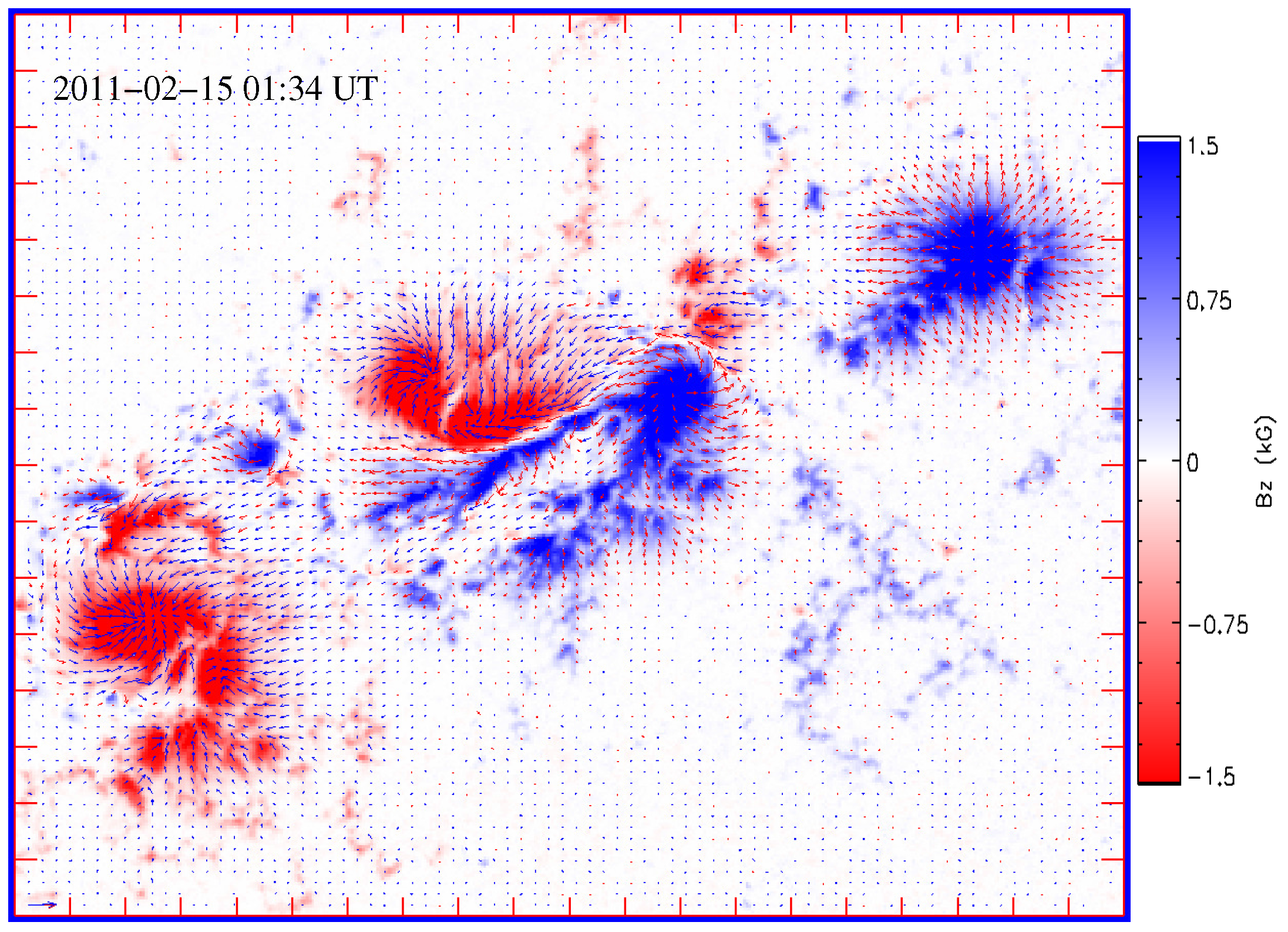
Figure 1. Non-potential (magnetic) field calculation (NPFC)-disambiguated vector magnetogram of NOAA active region (AR) 11158. The magnetogram is the closest preflare one to the X2.2 flare triggered in the AR (i.e., corresponding to the upper-left line-of-sight (LOS) magnetogram inset of Figure 2). The heliographic field components on the heliographic plane are shown. The vertical field strength has been saturated at ±1,500 G. The length of the blue vector at the lower-left corner corresponds to a horizontal field strength of 2,000 G. Tic mark separation is 10″. North is up; west is to the right.

Figure 1. Non-potential (magnetic) field calculation (NPFC)-disambiguated vector magnetogram of NOAA active region (AR) 11158. The magnetogram is the closest preflare one to the X2.2 flare triggered in the AR (i.e., corresponding to the upper-left line-of-sight (LOS) magnetogram inset of Figure 2). The heliographic field components on the heliographic plane are shown. The vertical field strength has been saturated at ±1,500 G. The length of the blue vector at the lower-left corner corresponds to a horizontal field strength of 2,000 G. Tic mark separation is 10″. North is up; west is to the right.

The following analysis uses the disambiguated heliographic magnetic field components deprojected onto the heliographic plane, tangential to the solar disk. This deprojection method neglects second-order corrections due to the solar curvature and relies on the Cartesian position-angle method of [26].

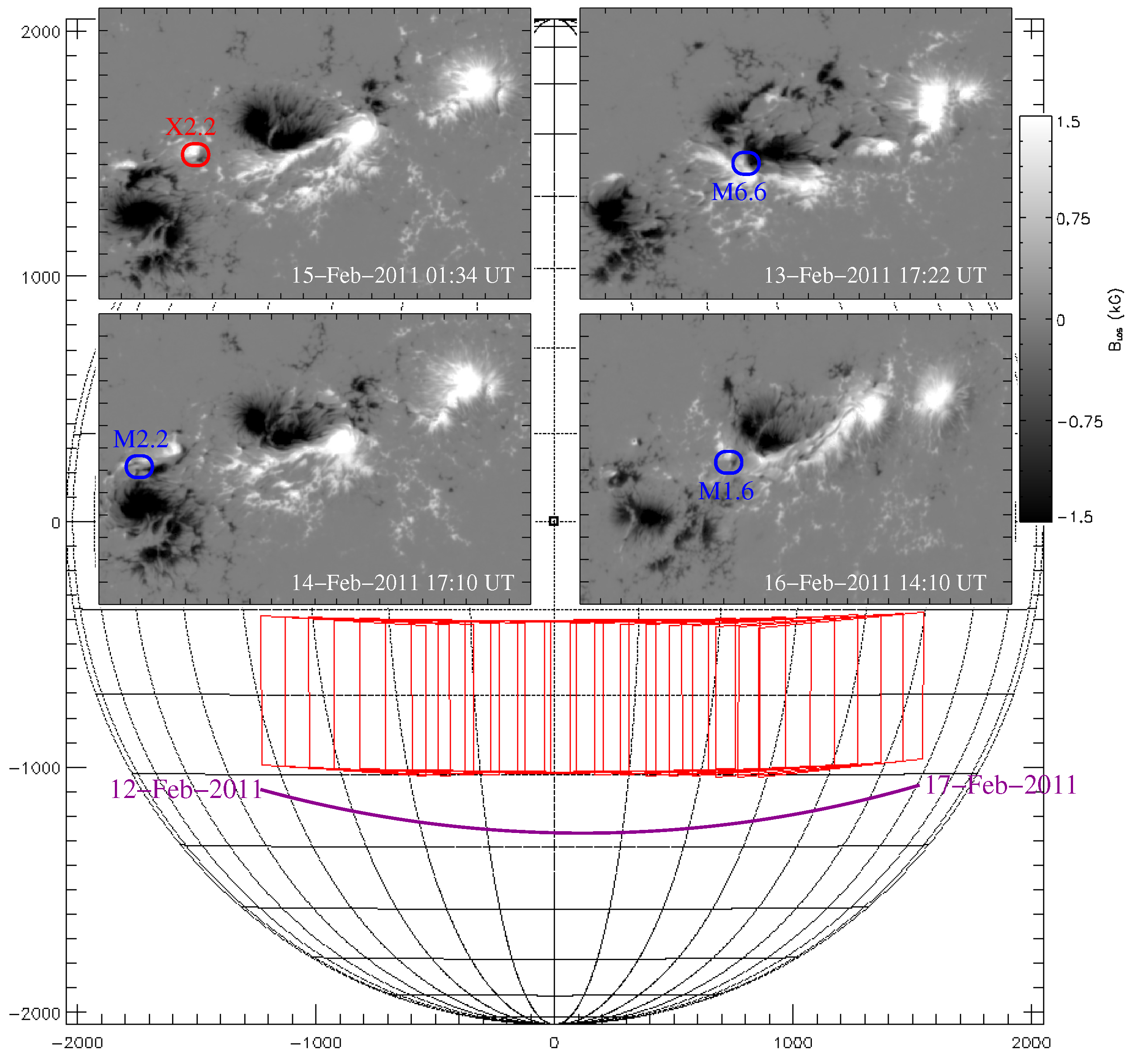
Following a near-quiescent evolution for most of February 12, 2011, NOAA AR 11158 started evolving rapidly late on that day, forming a dynamical quadrupolar magnetic configuration and featuring a strong, shear-ridden magnetic polarity inversion line (PIL). Figure 2 (background) shows the observed SDO/HMI cutout FOVs of the AR on the solar disk. For the purposes of this study, we focused on the four largest flares hosted by the AR between February 12 and 17, 2011, namely X2.2, M6.6, M2.2 and M1.6. The closest preflare line-of-sight (LOS) magnetograms of the AR are shown as insets in Figure 2. The flare sizes and approximate onset locations are indicated on each magnetogram, while a summary of the flare properties is provided in Table 1. For the flare locations, we used the Flare Detection module of the SDO Feature Finding Team (SDO/FFT) project [27] as reported in the Heliophysics Events Knowledgebase (HEK) [28].

Figure 2. Locations of NOAA AR 11158 on the solar disk over the five-day observing interval and respective major-flare locations within the AR (inset images). Shown in the background (red rectangles) are the field-of-view (FOV) locations of the SDO/HMI cutout vector magnetograms. The solar disk center is represented by the thick square. For clarity, one FOV every 2 h is shown. The four inset images show the LOS field components of the closest preflare magnetogram. Part of the cutout FOV has been removed in all cases for better focusing on the AR. Approximate flare onset locations are indicated by blue (M-class) and red (X-class) ovals. In all inset images, the LOS component is saturated at $\pm \mathrm{1,500}$ G. Tic mark separation 10″. North is up; west is to the right.

Figure 2. Locations of NOAA AR 11158 on the solar disk over the five-day observing interval and respective major-flare locations within the AR (inset images). Shown in the background (red rectangles) are the field-of-view (FOV) locations of the SDO/HMI cutout vector magnetograms. The solar disk center is represented by the thick square. For clarity, one FOV every 2 h is shown. The four inset images show the LOS field components of the closest preflare magnetogram. Part of the cutout FOV has been removed in all cases for better focusing on the AR. Approximate flare onset locations are indicated by blue (M-class) and red (X-class) ovals. In all inset images, the LOS component is saturated at $\pm \mathrm{1,500}$ G. Tic mark separation 10″. North is up; west is to the right.

Table 1. Synopsis of the three M- and one X-class flares selected for this study. Shown are the recently standardized solar object locators (SOL) for each event, as given in HEK, the GOES flare type, details of the flare temporal profile and the approximate flare location in $arcsec$ from the disk center (XY) and heliographic coordinates, namely central meridian distance (CMD) and latitude (LAT).

Solar Object Locator	GOES type	GOES universal time (UT)			HEK approximate flare location
		Onset	Peak	End	XY (arcsec)		CMD/LAT (deg)
SOL2011-02-15T01:44	X2.2	01:44	01:46	02:06	156	−226	9.86	−20.16
SOL2011-02-13T17:28	M6.6	17:28	17:38	17:47	−84	−226	−5.25	−20.09
SOL2011-02-14T17:20	M2.2	17:20	17:26	17:32	58	−231	3.63	−20.45
SOL2011-02-16T14:19	M1.6	14:19	14:25	14:29	468	−240	30.78	−20.19

Table 1. Synopsis of the three M- and one X-class flares selected for this study. Shown are the recently standardized solar object locators (SOL) for each event, as given in HEK, the GOES flare type, details of the flare temporal profile and the approximate flare location in $arcsec$ from the disk center (XY) and heliographic coordinates, namely central meridian distance (CMD) and latitude (LAT).

Solar Object Locator	GOES type	GOES universal time (UT)			HEK approximate flare location
		Onset	Peak	End	XY (arcsec)		CMD/LAT (deg)
SOL2011-02-15T01:44	X2.2	01:44	01:46	02:06	156	−226	9.86	−20.16
SOL2011-02-13T17:28	M6.6	17:28	17:38	17:47	−84	−226	−5.25	−20.09
SOL2011-02-14T17:20	M2.2	17:20	17:26	17:32	58	−231	3.63	−20.45
SOL2011-02-16T14:19	M1.6	14:19	14:25	14:29	468	−240	30.78	−20.19

3. Classes of Flare-Predictive Diagnostics

3.1. Multiscale Parameters

Calculation of the multiscale parameters described below does not require vector magnetograms. For this purpose, we have used the heliographic-plane deprojected vertical component, $B_z$, of each SDO/HMI magnetogram (e.g., the background of Figure 1).

Monoscale (fractal) and multiscale (multifractal) methods exploit the notions of scale-invariance, turbulence and intermittency, which have been long known to exist in solar magnetic structures (see, e.g., [5,8,29,30,31,32]). For a discussion of these methods and the promise they have delivered for an efficient flare prediction, the reader is referred to [4] and the references therein. From the existing array of parameters, we choose, as in that study, three of the most prominent ones, namely: (i) the fractal dimension, $D_0$; (ii) the power-law scaling index, α, of the turbulent power spectrum; and (iii) the multifractal structure-function, $S_q\left(r\right)$, for various displacements $\mathbf{r}$ and selector q. These methods are briefly explained in the following:

Covering the FOV of a given magnetogram with a square mesh of linear size L, linear size λ per individual mesh box (size element) and respective dimensionless size $\epsilon =\lambda /L$, the entire FOV is covered by ${(L/\lambda )}^2={(1/\epsilon )}^2$ boxes. To cover a structure that does not occupy the entire FOV, one needs a number $N\left(\epsilon \right)<{(1/\epsilon )}^2$ of elementary boxes. If we change the size element, λ and, hence, the dimensionless size, ε, at will, the respective number, $N\left(\epsilon \right)$, of boxes needed will vary accordingly. In this sense, we obtain a scaling relation:

$$N\left(\epsilon \right)\propto {(1/\epsilon )}^{D_0}$$

(1)

where $D_0$ is the scaling exponent. If there is a spatial scale invariance within the studied magnetic structure, then the scaling index, $D_0$, known as the (box counting) fractal dimension, will assume a non-integer value. The maximum possible value of $D_0$ is the non-fractal, Euclidean dimension of the structure (two in our case, as explained above). In the great majority of cases, for a two-dimensional fractal, we have $1<D_0<2$, although it is not impossible to have $D_0<1$ in the case of a very scarce filling by small, dust-like “islands”.

To practically calculate $D_0$ for the SDO/HMI magnetograms of our set, we must first subject $B_z$ to spatial and/or temporal thresholding. Calculation is performed for the part of the structure that exceeds the threshold(s). We first apply a $|B_z|$-threshold of 200 G that leaves a number of $B_z$-“islands” within the FOV. For each of these “islands” of area S, we apply: (i) a threshold imposing a minimum number of pixels, equal to 10; and (ii) a minimum magnetic-flux ${\Phi }_{min}=\int \left|B_z\right|dS$ threshold, equal to ${10}^{19}$ Mx. A further minimum threshold of 20 boundary pixels is applied for each of the otherwise qualifying islands. The thresholding aims to exclude, to the extent possible, quiet-Sun magnetic structures from the studied FOV.

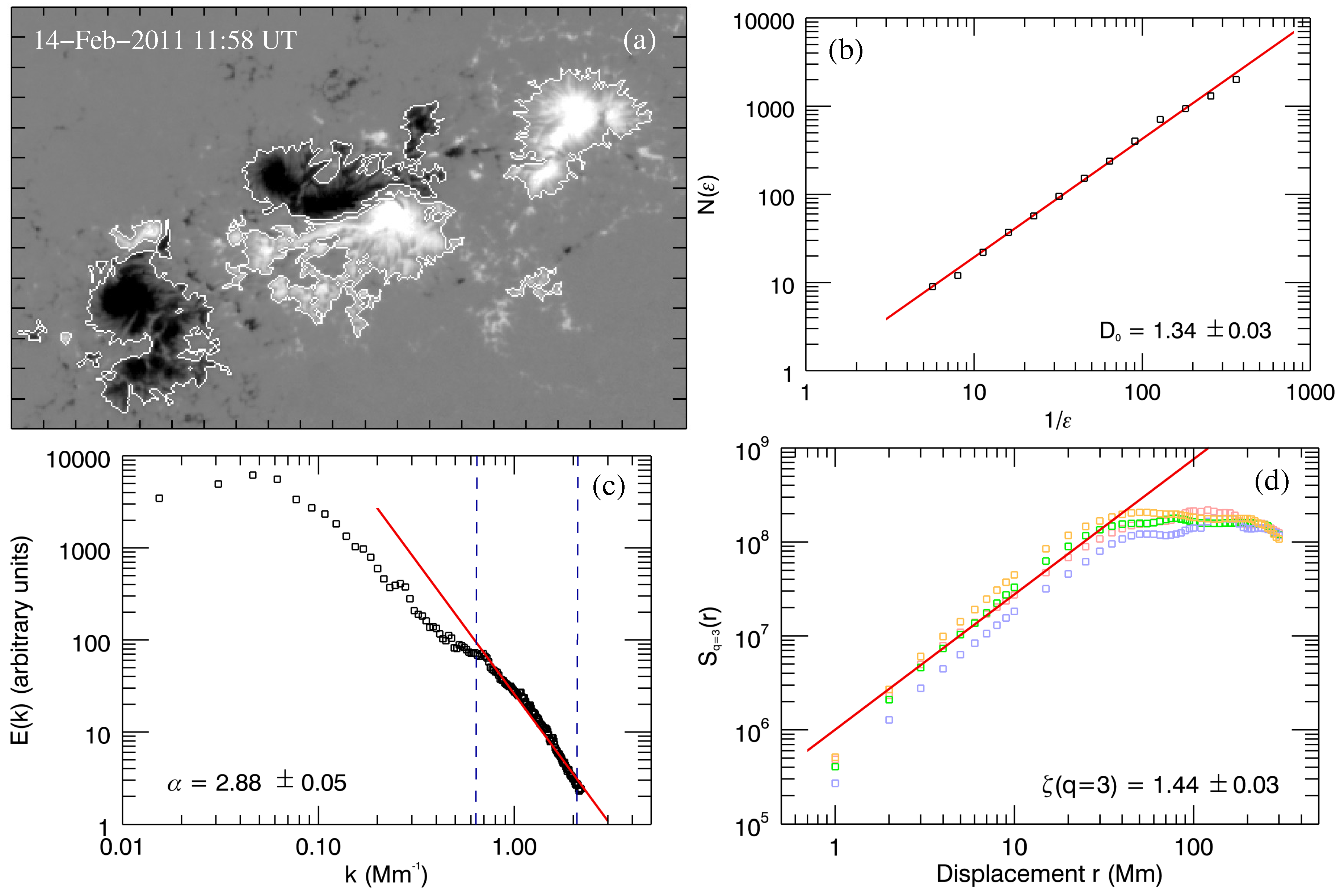
The number, $N\left(\epsilon \right)$, of boxes needed to calculate the fractal dimension may include either the interior of the qualifying $B_z$-islands or just their outline. As in various studies of solar magnetic fields, including [4,32], we follow the latter approach. An example calculation of the fractal dimension, $D_0$, via Equation (1) for the magnetogram of Figure 3a is shown in Figure 3b. The studied outlines are the white contours in Figure 3a.

Next, we investigate the turbulent power spectrum, $E\left(k\right)$, for an array of wavenumbers $k=2\pi /\ell$ associated with an array of length scales, ℓ. Turbulence develops in a hierarchy of scales in plasmas with high magnetic Reynolds numbers, which is the case for the solar atmosphere ([33,34]). If the studied structure is the outcome of turbulent evolution for a given length scale-range, then $E\left(k\right)$ should exhibit a power-law scaling behavior of the form:

$$E\left(k\right)\propto k^{-\alpha }$$

(2)

for the respective wavenumber-range, with a scaling exponent, α. The equivalent ℓ-range is interpreted as the turbulent inertial range of the structure, beyond which ($k>k_{max}$) non-ideal phenomena dissipate energy, thus interrupting the largely conservative inertial range. The author of [33] suggested that a reasonable inertial range for photospheric magnetic fields lies between $3<\ell <10$ Mm. We have followed this suggestion here, inferring α exclusively from this range. Notice that a value of $\alpha =5/3$ signals a classical hydrodynamic (HD) turbulence [35], while $\alpha =3/2$ corresponds to a theoretical intermittent magnetohydrodynamic (MHD) turbulence [36].

To infer α via Equation (2), we do not need a thresholded or otherwise partitioned $B_z$-map: the entire FOV can participate in the calculation. The result of this exercise for the magnetogram of Figure 3a is shown in Figure 3c. Notice that, indeed, for the k-range corresponding to $3<\ell <10$ Mm (dashed lines), there exists a scaling law implying that the magnetogram is modulated by turbulent action. Scaling is different than the one applying to larger-scale structures ($k<0.63M{m}^{-1}$). In addition, with $\alpha =2.88\pm 0.05$, the otherwise turbulent magnetogram exhibits neither HD (Kolmogorov) nor MHD (Kraichnan) turbulence.

The final multiscale parameter we apply is the multifractal structure-function spectrum, $S_q\left(r\right)$ ([29,37]). This parameter correlates the magnetic-flux distribution within the studied active region: for a given position, ${\mathbf{r}}_0$, in the magnetogram and a range, $\mathbf{r}$, of displacement vectors, it is given by:

$$S_q\left(r\right)=\langle |\Phi ({\mathbf{r}}_0+\mathbf{r})-\Phi \left({\mathbf{r}}_0\right){|}^q\rangle$$

(3)

Equation (3) implies that, to obtain $S_q\left(\mathbf{r}\right)$, one averages over all FOV locations, ${\mathbf{r}}_0$. Multifractality can be highlighted by raising the variation term to the q-power, where the selector, q, is typically an integer.

Figure 3. Example calculation of multiscale parameters on the median SDO/HMI magnetogram of our time series. (a) The heliographic vertical magnetic field component of the magnetogram, saturated at $\pm \mathrm{1,500}$ G. The white contours indicate the boundaries on which the fractal dimension, $D_0$, was calculated (see text). Tic mark separation 10″. North is up; west is to the right. (b) Calculation of the fractal dimension, $D_0$. The straight line corresponds to the least-squares best fit whose slope provides $D_0$. (c) Calculation of the turbulent power spectrum, $E\left(k\right)$, and respective least-squares best fit (red line) for the length scale-range [3, 10] Mm, indicated by the dashed blue lines. The slope of the fit provides α. (d) Calculation of the multifractal structure-function spectrum, $S_3\left(r\right)$, for a selector $q=3$. Different pale-colored spectra correspond to different displacement-vector orientations (north: red; south: green; east: blue; west; orange), while the straight line represents the mean least-squares best fit and its exponent, $\zeta \left(3\right)$.

Figure 3. Example calculation of multiscale parameters on the median SDO/HMI magnetogram of our time series. (a) The heliographic vertical magnetic field component of the magnetogram, saturated at $\pm \mathrm{1,500}$ G. The white contours indicate the boundaries on which the fractal dimension, $D_0$, was calculated (see text). Tic mark separation 10″. North is up; west is to the right. (b) Calculation of the fractal dimension, $D_0$. The straight line corresponds to the least-squares best fit whose slope provides $D_0$. (c) Calculation of the turbulent power spectrum, $E\left(k\right)$, and respective least-squares best fit (red line) for the length scale-range [3, 10] Mm, indicated by the dashed blue lines. The slope of the fit provides α. (d) Calculation of the multifractal structure-function spectrum, $S_3\left(r\right)$, for a selector $q=3$. Different pale-colored spectra correspond to different displacement-vector orientations (north: red; south: green; east: blue; west; orange), while the straight line represents the mean least-squares best fit and its exponent, $\zeta \left(3\right)$.

If intermittency is present in a magnetic-flux distribution, then for a range of displacement amplitudes, the spectrum $S_q\left(r\right)$ exhibits power-law scaling:

$$S_q\left(r\right)\propto r^{\zeta \left(q\right)}$$

(4)

where $\zeta \left(q\right)$ is the scaling index, regardless of the orientation of displacement, $\mathbf{r}$ [29,31]. The limiting case of a structure tested for intermittency is when $\zeta \left(q\right)=q/3$; in this case, no intermittency exists.

Similarly to the turbulent power spectrum and contrary to the fractal dimension, to calculate $S_q\left(r\right)$ and $\zeta \left(q\right)$, one does not need to subject the studied magnetogram to thresholding. The author of [38] suggested that a selector value $q=3$ is appropriate for active-region magnetograms, because it emphasizes the power-law regime of Equation (4). We follow this suggestion here and set $q=3$ hereafter. For the SDO/HMI magnetogram of Figure 3a, the calculation of $\zeta \left(3\right)$ is shown in Figure 3d. Shown with different symbol colors are the $S_3\left(r\right)$-spectra for four different displacement orientations: north, south, east and west. Notice the remarkably similar scaling, where each spectrum practically differs from the others by a simple multiplicative factor. This implies that the magnetogram of Figure 3a is indeed intermittent. A well-defined intermittency scaling index $\zeta \left(3\right)=1.44\pm 0.03$ is also obtained, which appears to be clearly different from its non-intermittency value $3/3=1$.

A detailed case study in [4] resulted in the scaling indices, α and $\zeta \left(q\right)$, being sensitive to the spatial resolution of the studied magnetogram, contrary to the fractal dimension, $D_0$, which remains roughly unaffected. The three different tested magnetograms referred to NOAA AR 10930 and were acquired by the low-resolution (full-disk) Michelson Doppler Imager (MDI) on board the Solar and Heliospheric Observatory (SOHO), the high-resolution SOHO/MDI and the Spectropolarimeter (SP) of the Solar Optical Telescope (SOT) on board Hinode. That study could not optimize a way of modeling the change of α- and $\zeta \left(q\right)$-values with spatial resolution. Hence, one cannot be fully confident about the values found in Figure 3c and Figure 3d and their deviation from HD/MHD turbulence and the lack of intermittency, respectively. In a further preliminary test, the multifractal Hurst exponent (for a discussion, see [39]) was calculated for the same three magnetograms [40]. A reasonable agreement was noted between the two highest-resolution magnetograms (high-resolution SOHO/MDI and Hinode SOT/SP), with the lowest-resolution magnetogram (low-resolution SOHO/MDI) differing significantly.

3.2. A Proxy Parameter

The effective connected magnetic field strength ($B_{eff}$) aims to quantify the single distinguishing feature of most eruptive solar active regions: their intense magnetic PIL at their lower (photospheric or chromospheric) boundary. The author of [1] characterized $B_{eff}$ as a morphological flare-predictive quantity, along with others, such as Schrijver’s [41] R, Falconer’s (e.g., [42] and the references therein) $W{L}_{SS}$ and $W{L}_{SG}$ parameters or the gradient-weighted inversion-line length (GWILL) [43]. All of these parameters weigh heavily on PILs, albeit with different specifics. In the present study, we characterize them as proxy quantities, because they should scale proportionally to fundamental physical quantities responsible for flares and eruptions, in general. These are the free magnetic energy and, arguably, the magnetic helicity of solar active regions. Indeed, PILs are responsible for dramatic increases of both quantities [44], so increased values of R, $B_{eff}$, $W{L}_{SS}$, $W{L}_{SG}$, GWILL and possibly others [45] should signal increased free-energy and relative-helicity budgets. This point is investigated later in this study.

The $B_{eff}$ metric, our proxy parameter of choice, also uses solely the vertical magnetic field component, $B_z$, of a magnetogram. It was introduced by [46]. That study concluded that $B_{eff}$ shows notable flare-predictive capability, and this was further justified by preliminary results shown in [1]. A more comprehensive statistical analysis is currently in preparation. Independent studies using $B_{eff}$ are also in progress ([47,48]).

Calculation of $B_{eff}$ relies on the magnetic-connectivity matrix of the studied active region (Figure 4). Given $N_{+}$ positive-polarity and $N_{-}$ negative-polarity magnetic-flux concentrations, or partitions, the connectivity matrix $\overline{\overline{\Phi }}=\left[{\Phi }_{ij}\right]$ is a $N_{+}\times N_{-}$ matrix containing all unsigned fluxes ${\Phi }_{ij}$ connecting the i-positive-polarity with the j-negative-polarity partition ($i\equiv \{1,...,N_{+}\}$; $j\equiv \{1,...,N_{-}\}$). Magnetic-flux partitioning relies on a flux-tessellation scheme used for topological studies [49] and is also described in detail in [50]. Assuming a respective matrix $\overline{\overline{L}}=\left[L_{ij}\right]$ containing the flux-weighted centroid distances, $L_{ij}$, between opposite-polarity partition pairs, $(i,j)$, then $B_{eff}$ is a scalar with magnetic-intensity units given by:

$$B_{eff}=\sum _{i=1}^{N_{+}}\sum _{j=1}^{N_{-}}\frac{{\Phi }_{ij}}{{L_{ij}}^2}$$

(5)

Mathematically, inference of $B_{eff}$ collapses all dipolar connections in a magnetogram into a single idealized connection rooted in two adjacent area elements (pixels). Then, $B_{eff}$ is the absolute vertical-field component at each of the two footpoints of the dipole.

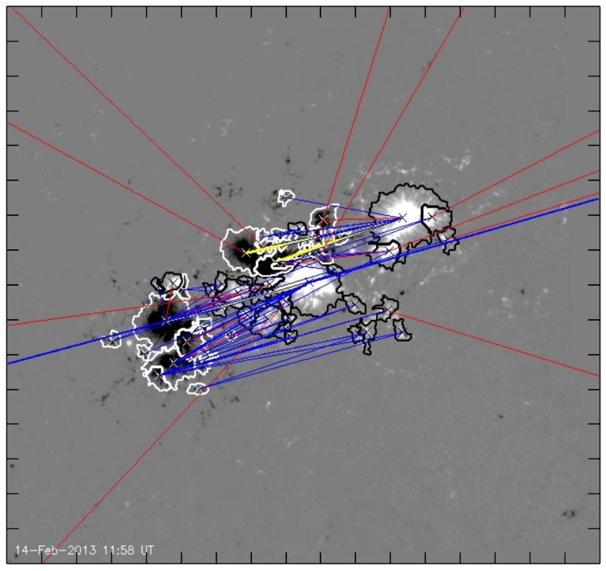
Figure 4. Connectivity-matrix calculation for the magnetogram of Figure 3a using a minimum partition size of 40 pixels and a flux threshold of $5\times {10}^{19}$ Mx. Individual magnetic connections are shown by colored line segments connecting the flux-weighted centroids of these partitions (crosses). Connections that reach to the edges of the FOV are considered “open”, namely closing beyond the confines of the AR. Red, blue and yellow segments denote unsigned connected fluxes in the range $(0.5,5)\times {10}^{20}$ Mx, $(5,10)\times {10}^{20}$ Mx and $(10,50)\times {10}^{20}$ Mx, respectively. The resulting $B_{eff}$-value in this case is 581.4 G. Tic mark separation is 20″.

Figure 4. Connectivity-matrix calculation for the magnetogram of Figure 3a using a minimum partition size of 40 pixels and a flux threshold of $5\times {10}^{19}$ Mx. Individual magnetic connections are shown by colored line segments connecting the flux-weighted centroids of these partitions (crosses). Connections that reach to the edges of the FOV are considered “open”, namely closing beyond the confines of the AR. Red, blue and yellow segments denote unsigned connected fluxes in the range $(0.5,5)\times {10}^{20}$ Mx, $(5,10)\times {10}^{20}$ Mx and $(10,50)\times {10}^{20}$ Mx, respectively. The resulting $B_{eff}$-value in this case is 581.4 G. Tic mark separation is 20″.

A given connectivity matrix corresponds to a given $B_{eff}$-solution. The connectivity matrix, furthermore, is sensitive to flux partitioning. To infer the flux partitions, we have imposed a minimum tolerated flux per partition and a minimum tolerated partition size, in terms of the number of pixels. The values used are $5\times {10}^{19}$ Mx and 40, respectively. These choices involve ∼70% of the total unsigned flux included in Figure 4 and certainly the strongest flux accumulations in the AR. Next, to calculate the connectivity matrix, we use a simulated-annealing technique [51] that minimizes a fractional, $\mathcal{R}$, of the form:

$$\mathcal{R}=\sum (\frac{|{\mathbf{r}}_a-{\mathbf{r}}_b|}{R_{max}}+\frac{|{\Phi }_a+{\Phi }_b|}{|{\Phi }_a|+|{\Phi }_b|})$$

(6)

where ${\Phi }_a$ and ${\Phi }_b$ are the signed fluxes of partitions a and b and ${\mathbf{r}}_a$ and ${\mathbf{r}}_b$ are the vector positions of their respective flux-weighted centroids. Moreover, $R_{max}$ is the maximum possible length within the magnetogram, namely its diagonal length. The sum in Equation (6) corresponds to all possible $(a,b)$-pairs. Physically, this practice aims to connect opposite-polarity partitions emphasizing the ones that are most closely spaced. The problem is numerically complex with numerous local minima for $\mathcal{R}$, hence the simulated annealing, which is an iterative process known to asymptotically achieve the global minimum of $\mathcal{R}$ when the number of iterations tends to infinity.

Criticism on the simulated-annealing calculation of the connectivity matrix and, by extension, on the inference of $B_{eff}$ has been drawn by [2]. This criticism was addressed in detail by [1,12], so we will not discuss it further here.

The connectivity matrix corresponding to the magnetogram of Figure 3a is provided in Figure 4. From this, the calculation of $B_{eff}\simeq 581.4$ G is straightforward via Equation (5). Notice that $B_{eff}$ ignores the “open” flux connections; only flux connections closing within the FOV are included in the calculation.

3.3. Fundamental Physical Parameters

As discussed previously, the budgets of magnetic free energy and relative magnetic helicity in an active region correspond to fundamental physical quantities necessary for powering solar eruptions. If so, however, why should one rely on proxy parameters? The answer lies both on physical grounds and on the complicated nature of calculating credible free-energy and relative-helicity budgets. In the conventional calculations applied so far, one needs either a reliable flow velocity field in the (photospheric or chromospheric) boundary, where a time series of magnetograms has been obtained, or a reliable extrapolated three-dimensional magnetic field for each snapshot of the time series. Each extrapolated field is calculated using the respective snapshot of the magnetogram time series as the required boundary condition. Both approaches are known to be heavily affected by flow-field uncertainties ([52] and the references therein) and extrapolation-model-dependencies ([53,54,55]). In addition, even in the case that flow fields are precisely inferred, it remains to be clarified to what degree do peculiar motions in the active-region photosphere truly relate to the injection of sufficient magnetic energy and helicity budgets from deep in the convection zone to power a major flare or merely reflect solar surface-dynamo processes [56].

The problem of a seamless calculation of magnetic free-energy and relative magnetic-helicity budgets in solar active regions was tackled by [12], who developed a nonlinear force-free method to self-consistently calculate a minimum free-energy budget and the corresponding relative-helicity budget. The calculation does not require flow fields, time series of magnetograms or three-dimensional extrapolated fields. A single vector magnetogram can give rise to a pair of instantaneous free-energy and relative-helicity budgets. A time series of vector magnetograms leads to a pseudo-time series of free-energy and relative-helicity budgets, where each value is independent of prior or posterior values. This is a generalization of the initial linear force-free approach to the problem [57]. The nonlinear force-free treatment utilizes “closed” magnetic connections in connectivity matrices, such as the one of Figure 4. The connectivity matrix is now viewed as a collection of, say, N slender force-free flux tubes, each with an unsigned flux content, ${\Phi }_m$, and a force-free parameter, ${\alpha }_m$, where $m\equiv 1,...,N$. The interaction between these flux tubes determines the form of the connectivity matrix and, by extension, the respective free energy and helicity budgets, namely [12]:

$$E_c=A{\lambda }^2\sum _{m=1}^N{\alpha }_m^2{\Phi }_m^{2\delta }+\frac{1}{8\pi }\sum _{m=1}^N\sum _{n=1;m\ne n}^N{\alpha }_m{\mathcal{L}}_{mn}^{arch}{\Phi }_m{\Phi }_n,and$$

(7)

$$H_{mag}=8\pi A{\lambda }^2\sum _{m=1}^N{\alpha }_m{\Phi }_m^{2\delta }+\sum _{m=1}^N\sum _{n=1;m\ne n}^N{\mathcal{L}}_{mn}^{arch}{\Phi }_m{\Phi }_n$$

(8)

for the free magnetic energy, $E_c$, and the relative magnetic helicity, $H_{mag}$, respectively. In Equations (7) and (8), A and δ are known fitting constants, λ is the size element (pixel size) of the magnetogram and ${\mathcal{L}}_{mn}^{arch}$; $m\ne n$, is the mutual-helicity factor of flux tubes m and n, which are not supposed to wind around each other. The latter is a geometrical parameter fully determined for any couple of known footpoint pairs of two slender flux tubes. The explicit omission of a respective Gauss linking number, ${\mathcal{L}}_{mn}^{close}$, due to the intertwining between different flux tubes, which would require knowledge of the exact three-dimensional magnetic configuration, is the reason for obtaining a minimum free energy, $E_c$, for the given connectivity matrix. This method, therefore, assumes ${\mathcal{L}}_{mn}^{close}=0$ for each pair $(m,n)$; $m\ne n$ of flux tubes. Furthermore, in Equations (7) and (8), ${\Phi }_m\equiv {\Phi }_{ij}$, that is, it is the flux connecting the partition pair $(i,j)$ discussed in the previous Section. The force-free parameter, ${\alpha }_m\equiv {\alpha }_{ij}$, of each flux tube is the mean value of the two force-free parameters, ${\alpha }_i$ and ${\alpha }_j$, of partitions i and j, respectively. A partition’s flux-weighted force-free parameter is calculated by substituting its total electric current, $I_a$, and respective flux content, ${\Phi }_a$, into the integral expression of Ampere’s law, as explained by [12].

For the connectivity matrix of Figure 4, we find $E_c\simeq 1.2\times {10}^{32}$ erg and $H_{mag}\simeq 2.3\times {10}^{43}M{x}^2$.

4. Results and Discussion

4.1. Parameter Time Series over the Observing Interval

Using the methods described in Section 3, we now calculate the selected multiscale, proxy and fundamental physical parameters for each of the 600 magnetograms of NOAA AR 11158. To our understanding, there are few studies (see, e.g., [31] for a study of multiscale parameters) that perform this test for such a high-cadence, days-long time series, particularly for proxy and fundamental physical parameters.

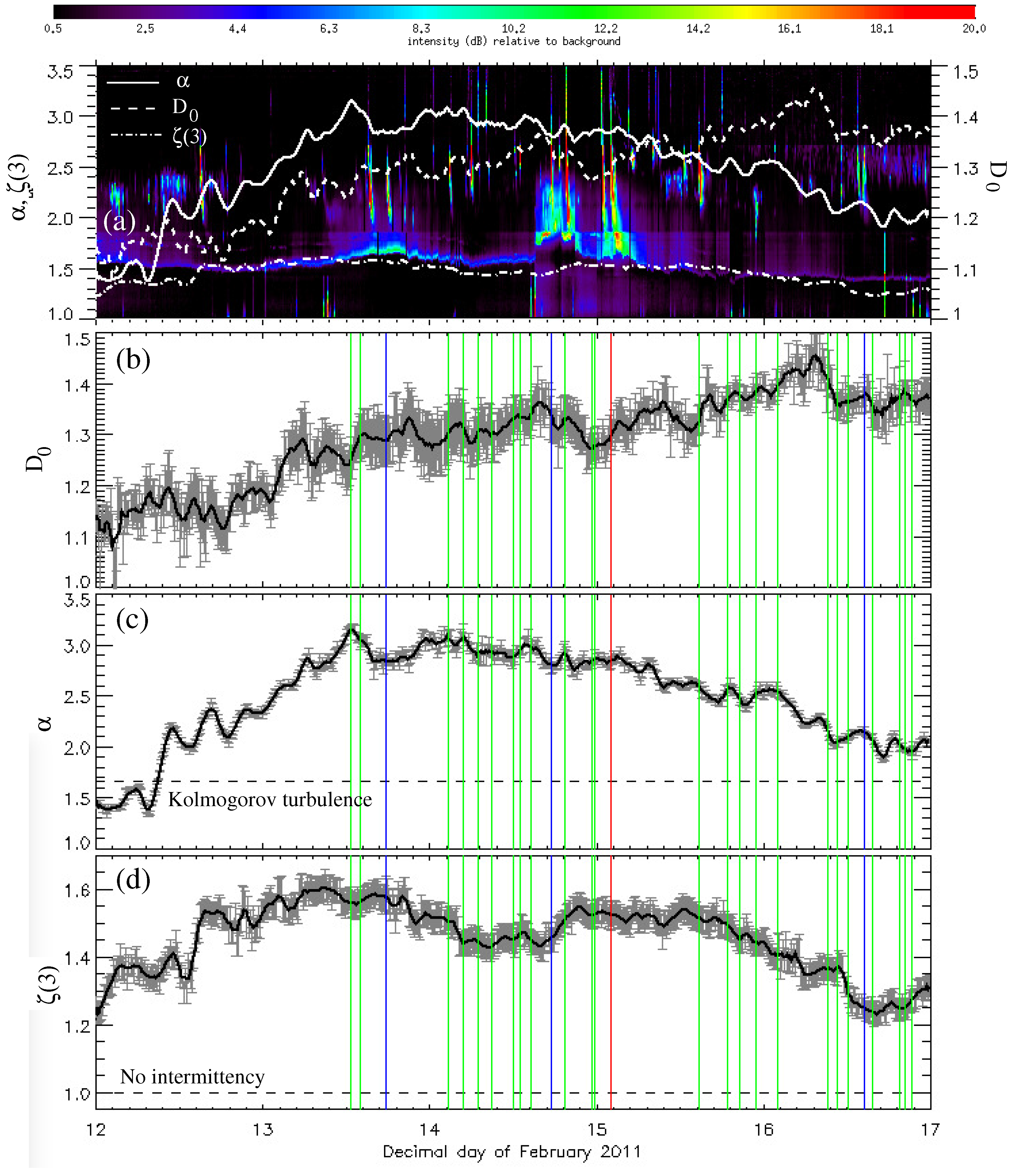
For multiscale parameters, the results are shown in Figure 5. The background of Figure 5a provides the solar frequency-time radio spectrum within the same five-day period of interest, as obtained by the Waves instrument [58] on board the Wind mission. This spectrum complements the picture with a meaningful physical context, because it highlights shock-fronted CMEs, with shocks typically appearing as Type II bursts [59]. However, the Wind/Waves instrument does not have spatial resolution, thus registering indiscriminately events from the entire Sun. For this reason, Figure 5b–d corresponding to the time series of the fractal dimension, $D_0$, scaling index α of the turbulent power spectrum, and intermittency scaling index $\zeta \left(3\right)$, respectively, include the onset times of flares, ≥$C1.0$, triggered exclusively in NOAA AR 11158. Apparently, the temporal association of a flare with a Type II burst is only an indication that the flare is eruptive. Confirmation or dismissal of this hypothesis can only be achieved via examination of X-ray and/or extreme ultraviolet (EUV) images of the flare, as well as of existing CME databases (the main SOHO Large Angle and Spectrometric Coronagraph (LASCO) one [60], but also the Solar Eruptive Event Detection System (SEEDS) [61] and the Computer-Aided CME Tracking (CACTus) [62]) databases, providing precise location estimates of the CME source.

The time series of the tested multiscale parameters show overall consistency, but distinct morphological features. In particular:

(1)

The fractal dimension, $D_0$, (Figure 5b) shows a generally increasing trend throughout the entire interval. This trend is reminiscent of the increasing trend shown either by the total unsigned flux in the AR (see Figure 2 of [20]) or that of the total connected flux, $\sum {\Phi }_{ij}$, in the connectivity matrix (Figure 6a). This implies that $D_0$ may be directly proportional to the active-region flux, which is a result suggested by other studies, as well [63].

(2)

The scaling index, α, (Figure 5c), on the other hand, reaches a peak fairly early in the AR evolution (decimal days 13.5–14) and then starts decreasing nearly monotonically for the rest of the observing interval. Recalling that the flux in the AR is generally increasing in the same interval, this means that from February 14th onwards, turbulence in the AR becomes more robust, forming a “harder”, better established inertial range and moving toward “nominal” Kolmogorov values. The AR has yet to reach these values by the end of the observing period. Overlooking the dependence of α on spatial resolution [4], therefore, one would argue that the AR is characterized by non-Kolmogorov/non-Kraichnan turbulence for the entire observing interval. Only at very initial stages (decimal day ≤$12.5$) do we obtain α-values closer to Kraichnan turbulence ($\alpha \sim 1.5$). Further work on high-cadence data and, ideally, ARs observed from emergence to decay is required to understand this effect and its meaning; it might be that ARs start with a turbulence closer to MHD intermittent or HD values, but, in the course of their evolution, closely interacting magnetic partitions quickly quench this picture toward more complex patterns. In [4], virtually all studied ARs, be they flaring or non-flaring, show α-values far from the range $(1.5,1.667)$. The authors of [34], on the other hand, seem to obtain α-values closer to this range mostly for unipolar sunspots and decaying ARs.

(3)

The intermittency index, $\zeta \left(3\right)$, fluctuates around values 1.5–1.6 for most of the observing interval, namely between decimal days 12.6 and 15.6. For about a day, between days 14 and 15, we notice a significant decrease reaching up to values ∼1.4. Before decimal days 12.6 and after 15.6, $\zeta \left(3\right)$-values are lower, around ∼1.4 for the former and nearly monotonically decreasing for the latter intervals, respectively. The decrease between decimal days 15.6 and 16.7 seems steeper than that of α, while for the last 8 h of the observing interval (decimal day >16.7) $\zeta \left(3\right)$-values consistently start increasing again. At no time during the observing interval does $\zeta \left(3\right)$ become lower than 1.2, which means that, again overlooking the spatial-resolution dependence reported by [4], the magnetic field of the AR shows significant intermittency.

Figure 5. Time series of multiscale parameters for the five-day observing interval of NOAA AR 11158. (a) Results overplotted against the respective Wind/Waves frequency-time radio spectrum ranging logarithmically between five and ${10}^4$ kHz. The color scale shows intensity with respect to the background. (b) Fractal-dimension time series (dashed line in a) with the thick black curve showing 72-min averaged values and gray indicating actual $D_0$-values and their uncertainties (error bars). (c) Turbulent scaling-index time series (solid line in a) with the thick black curve showing 72-min averaged values and gray indicating actual α-values and respective uncertainties. The dashed line indicates the α-value of Kolmogorov’s hydrodynamic (HD) turbulence. (d) Intermittency scaling index (dash-dotted line in a) with the thick black curve showing 72-min averaged values and gray indicating actual $\zeta \left(3\right)$-values and respective uncertainties. The dashed line indicates the $\zeta \left(3\right)$-value in the absence of intermittency. Colored line segments in b–d correspond to the GOES 1–8 ÅX-ray onset times of flares triggered in the AR, with green, blue and red denoting C-, M- and X-class flares, respectively.

Figure 5. Time series of multiscale parameters for the five-day observing interval of NOAA AR 11158. (a) Results overplotted against the respective Wind/Waves frequency-time radio spectrum ranging logarithmically between five and ${10}^4$ kHz. The color scale shows intensity with respect to the background. (b) Fractal-dimension time series (dashed line in a) with the thick black curve showing 72-min averaged values and gray indicating actual $D_0$-values and their uncertainties (error bars). (c) Turbulent scaling-index time series (solid line in a) with the thick black curve showing 72-min averaged values and gray indicating actual α-values and respective uncertainties. The dashed line indicates the α-value of Kolmogorov’s hydrodynamic (HD) turbulence. (d) Intermittency scaling index (dash-dotted line in a) with the thick black curve showing 72-min averaged values and gray indicating actual $\zeta \left(3\right)$-values and respective uncertainties. The dashed line indicates the $\zeta \left(3\right)$-value in the absence of intermittency. Colored line segments in b–d correspond to the GOES 1–8 ÅX-ray onset times of flares triggered in the AR, with green, blue and red denoting C-, M- and X-class flares, respectively.

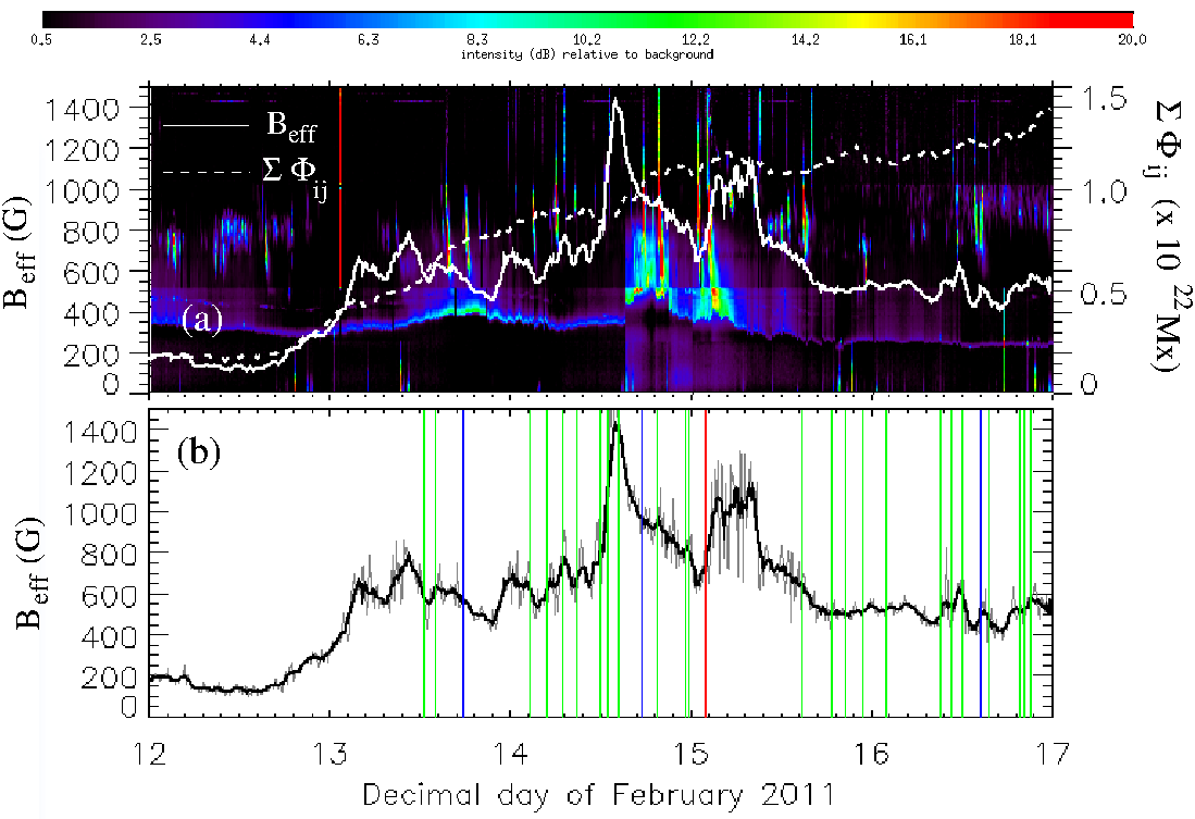
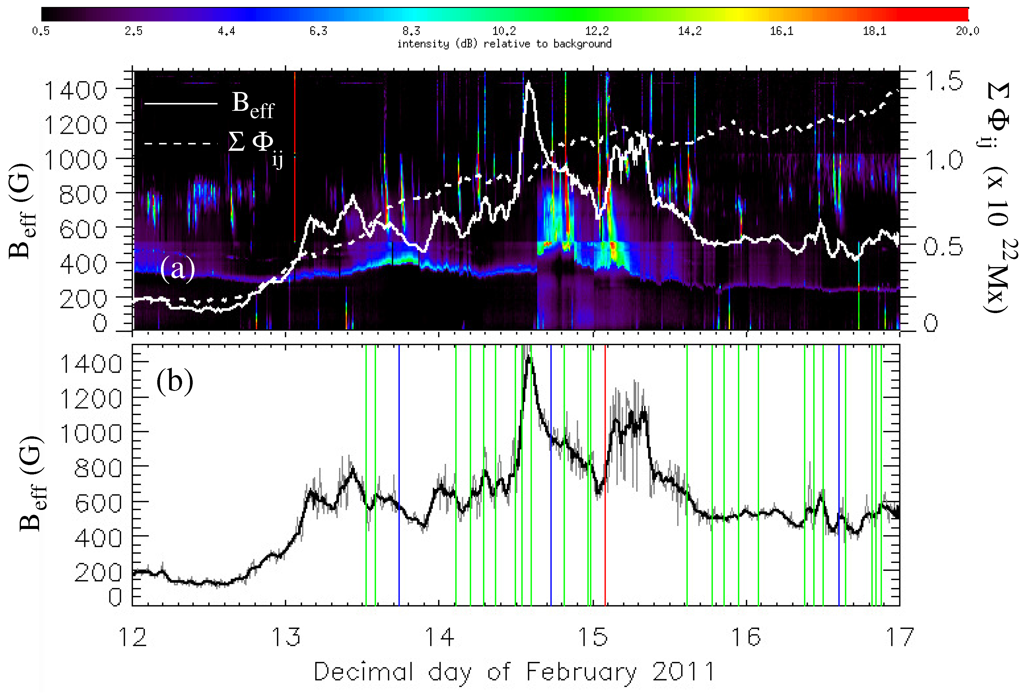
The time series of the chosen proxy parameter, $B_{eff}$, is provided in Figure 6. We notice here a more distinctive $B_{eff}$-pattern than those of multiscale parameters: up until decimal day 12.7, $B_{eff}$-values are very low ($\le 200$ G); the abrupt increase of the total connected flux (Figure 6a) thereafter, however, enhances $B_{eff}$ significantly. From decimal day 13.1 onwards, one may roughly describe the temporal evolution of $B_{eff}$ as the superposition of two distinct elements: a “background” value of $B_{eff}\simeq 500$ G and impulsive $B_{eff}$-enhancements followed by more gradual decreases to, or close to, the background value. We notice a number of C-class flares close to the background value, but the major flares in the AR (1 X-class; 3 M-class) seem to be occurring during the decaying phase of $B_{eff}$-impulses. The most conspicuous and abrupt of these impulses precedes the M2.2 and X2.2 flares of Table 1. This effect is discussed in more detail in Section 4.2.

Figure 6. Time series of the proxy parameter, $B_{eff}$, for the five-day observing interval of NOAA AR 11158. (a) Results overplotted against the respective Wind/Waves frequency-time radio spectrum ranging logarithmically between five and ${10}^4$ kHz. The color scale shows intensity with respect to the background. The dashed curve corresponds to the total connected flux included in each connectivity matrix. (b) Effective connected magnetic field strength time series (solid line in a) with the thick black curve showing 72-min averaged values and gray indicating actual $B_{eff}$-values. Colored line segments correspond to the GOES 1–8 ÅX-ray onset times of flares triggered in the AR, with green, blue and red denoting C-, M- and X-class flares, respectively.

Figure 6. Time series of the proxy parameter, $B_{eff}$, for the five-day observing interval of NOAA AR 11158. (a) Results overplotted against the respective Wind/Waves frequency-time radio spectrum ranging logarithmically between five and ${10}^4$ kHz. The color scale shows intensity with respect to the background. The dashed curve corresponds to the total connected flux included in each connectivity matrix. (b) Effective connected magnetic field strength time series (solid line in a) with the thick black curve showing 72-min averaged values and gray indicating actual $B_{eff}$-values. Colored line segments correspond to the GOES 1–8 ÅX-ray onset times of flares triggered in the AR, with green, blue and red denoting C-, M- and X-class flares, respectively.

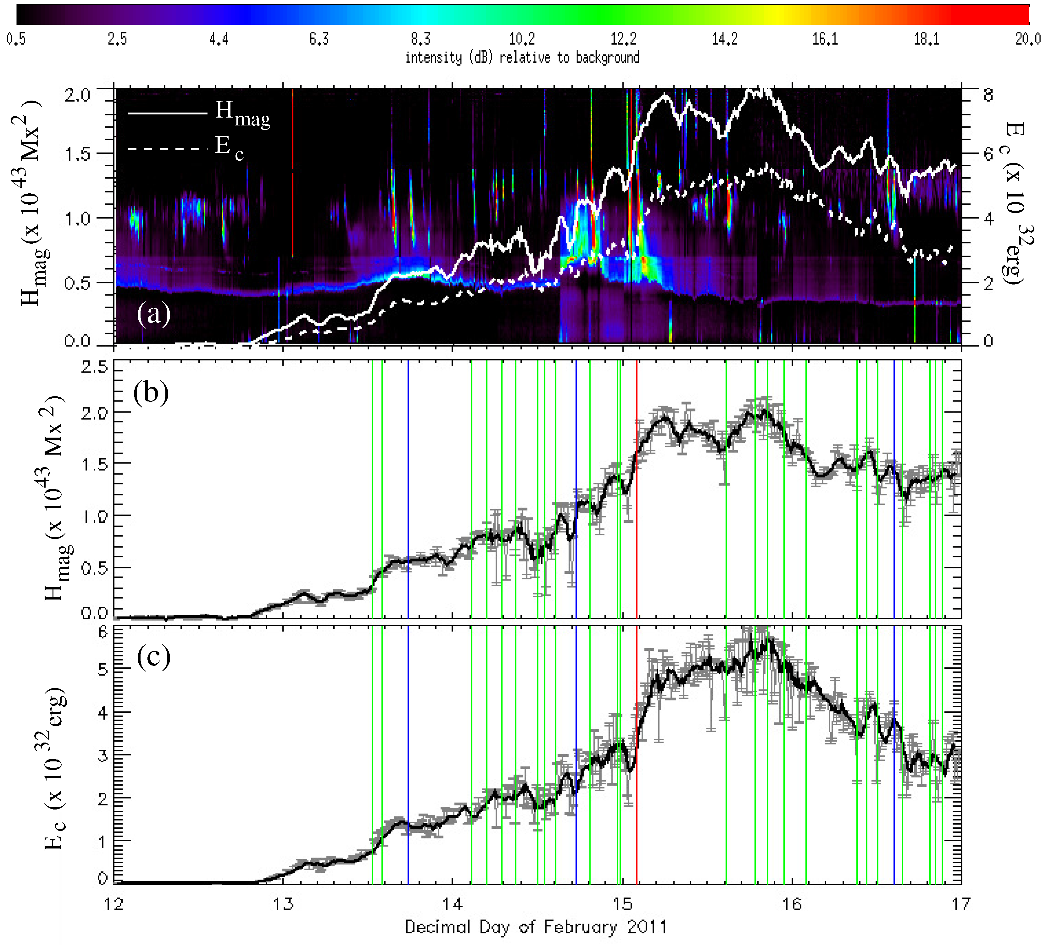
Finally, the time series of our fundamental physical parameters, namely the relative magnetic helicity, $H_{mag}$, and the magnetic free energy, $E_c$, are shown in Figure 7. This analysis was first performed by [20]. The self-consistent calculation of $H_{mag}$ and $E_c$ (Equations (7) and (8)) results in generally similar morphologies for both time series: a roughly linear, gradual increase of both quantities occurs between decimal days 12.8 and 15; this follows the similar increase of the total connected flux (Figure 6a). After decimal day 15.0, however, immediately following the X-class flare early on February 15, 2001, both $H_{mag}$ and $E_c$ start increasing abruptly. The relative helicity, $H_{mag}$, shows two peaks, both at ∼$2\times {10}^{43}M{x}^2$, at decimal days 15.2 and ∼$15.8$, after which it decreases until decimal day 16.2. Thereafter, it fluctuates around ∼$1.5\times {10}^{43}M{x}^2$. The magnetic free energy shows a single peak (∼$6\times {10}^{32}$ erg) at decimal day ∼$15.9$ and then decreases linearly to values <$3\times {10}^{32}$ erg at the end of the observing interval. The elements of this behavior for both $H_{mag}$ and $E_c$ have been extensively presented and discussed in Section 5 of [20].

Figure 7. Time series of fundamental physical parameters for the five-day observing interval of NOAA AR 11158. (a) Results overplotted against the respective Wind/Waves frequency-time radio spectrum ranging logarithmically between five and ${10}^4$ kHz. The color scale shows intensity with respect to the background. (b) Relative magnetic-helicity time series (solid line in a) with the thick black curve showing 72-min averaged values and gray indicating actual $H_{mag}$-values and their uncertainties (error bars). (c) Free magnetic-energy time series (dashed line in a) with the thick black curve showing 72-min averaged values and gray indicating actual $E_c$-values and respective uncertainties. Colored line segments in b and c correspond to the GOES 1–8 ÅX-ray onset times of flares triggered in the AR, with green, blue and red denoting C-, M- and X-class flares, respectively.

Figure 7. Time series of fundamental physical parameters for the five-day observing interval of NOAA AR 11158. (a) Results overplotted against the respective Wind/Waves frequency-time radio spectrum ranging logarithmically between five and ${10}^4$ kHz. The color scale shows intensity with respect to the background. (b) Relative magnetic-helicity time series (solid line in a) with the thick black curve showing 72-min averaged values and gray indicating actual $H_{mag}$-values and their uncertainties (error bars). (c) Free magnetic-energy time series (dashed line in a) with the thick black curve showing 72-min averaged values and gray indicating actual $E_c$-values and respective uncertainties. Colored line segments in b and c correspond to the GOES 1–8 ÅX-ray onset times of flares triggered in the AR, with green, blue and red denoting C-, M- and X-class flares, respectively.

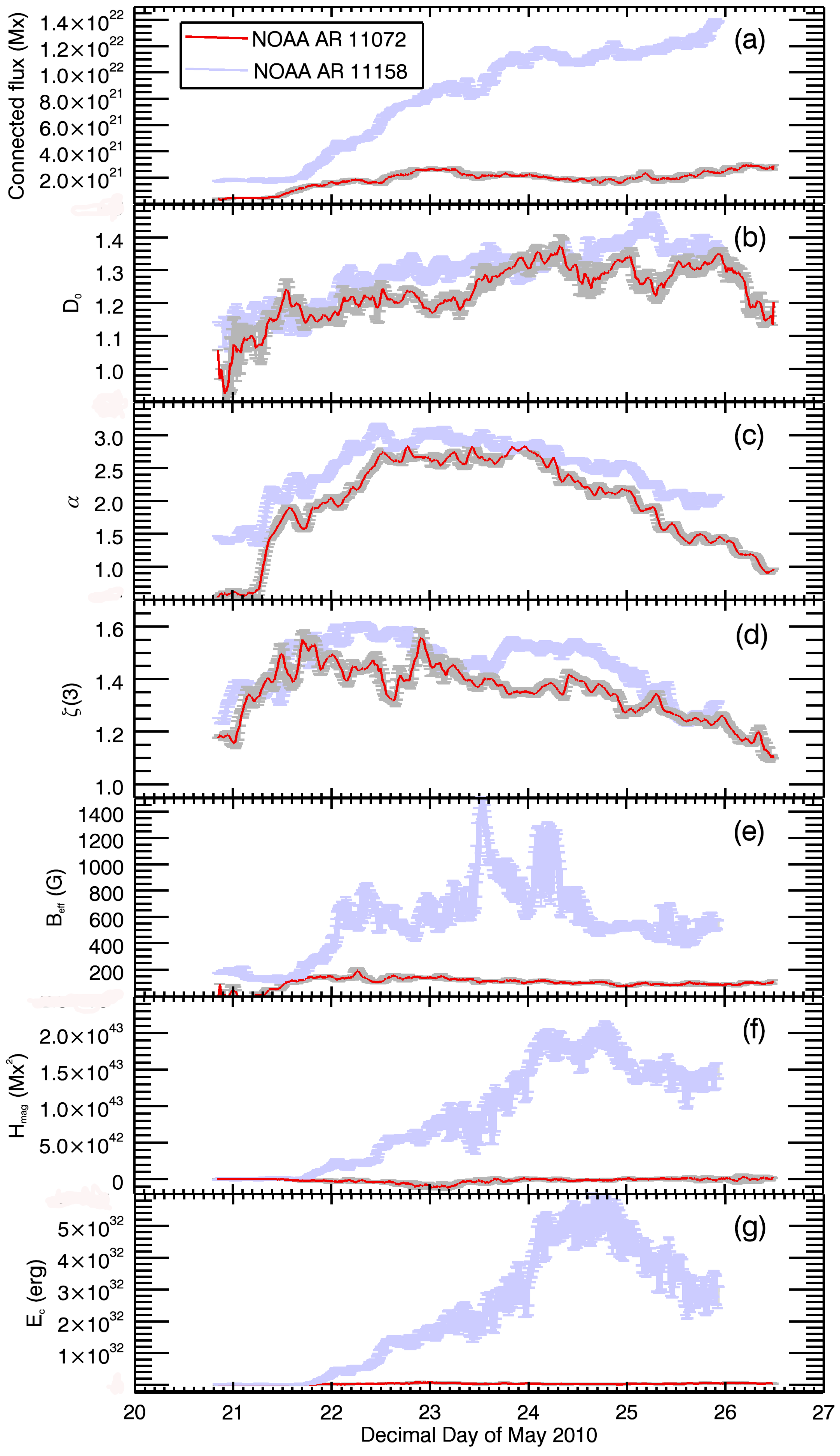
Before discussing the detailed features of the studied parameters around the times of major flares, it is instructive to compare the results of Figure 5, Figure 6 and Figure 7 to respective results obtained for a “quiescent”, non-eruptive solar active region. Browsing the database of released SDO/HMI cutout vector-magnetogram time series, we selected NOAA AR 11072, observed by the SDO/HMI for a ∼$5.5$-day period in May, 2010. As with NOAA AR 11158, NOAA AR 11072 was observed from emergence, late on May 20, 2010. The region maintained a basic dipolar configuration throughout the observing interval, with a compact leading sunspot and a more dispersed trailing one. The AR lacked a strong, sheared PIL. GOES detected only a few B-class flares as originating from the AR, while there was no sign of CMEs launched from the region. NOAA AR has been studied in detail in [64,65]. The AR’s 666 snapshot vector magnetograms were treated identically with those of NOAA AR 11158, as detailed in Section 2.

Figure 8 depicts the time series of the tested multiscale, proxy and fundamental physical parameters in NOAA AR 11072 (red curves; gray uncertainties) in comparison to the respective time series of NOAA AR 11158, originally shown in Figure 5, Figure 6 and Figure 7 (light blue curves and uncertainties). Figure 8 leads to two important conclusions: first, as also reported by [4] for a comprehensive active-region dataset, multiscale parameters between the intensely eruptive NOAA AR 11158 and the “quiescent” NOAA AR 11072 have fairly similar values (Figure 8b–d). The high cadence of the observations in this study reveals even similar morphologies for these time series. Second, NOAA AR 11072 has substantially lower values for proxy and fundamental physical parameters. As explained in Section 3.2 and Section 3.3, these parameters rely on the connected magnetic flux, $\sum {\Phi }_{ij}$ (Figure 8a): NOAA AR 11072 shows a connected flux that is 2–7 times smaller than that of NOAA AR 11158. This difference gives rise to: (i) a factor of 5–14-difference in the respective $B_{eff}$-values (for NOAA AR 11072, these range between 100 G and 200 G); (ii) a factor of ∼50-difference in average relative-helicity values (for NOAA AR 11072, these peak at ∼$3\times {10}^{41}$ Mx${}^2$); and (iii) a factor of ∼66-difference in average free-energy values (for NOAA AR 11072, these peak at ∼$8\times {10}^{30}$ erg). Clearly, therefore, one would be able to distinguish the eruptive from the non-eruptive AR by focusing solely on the $B_{eff}$-, $H_{mag}$- or $E_c$-values, or even on the $\sum {\Phi }_{ij}$-values. This task would not have been as straightforward had one focused on the $D_0$-, α- or $\zeta \left(3\right)$-values alone.

Figure 8. Comparison between NOAA AR 11158 and the non-eruptive active region NOAA AR 11072: time series of connected magnetic flux (a); multiscale parameters (b–d); proxy parameter (e); and fundamental physical parameters (f,g) for NOAA AR 11072 (red curves; gray uncertainties) observed by SDO/HMI over a ∼$5.5$ observing interval in May, 2010. The respective time series and uncertainties for NOAA AR 11158 are also shown (light blue), assumed as starting from the start of observations of NOAA AR 11072 and lasting five days thereafter. All shown curves are 72-min averages of the actual curves.

Figure 8. Comparison between NOAA AR 11158 and the non-eruptive active region NOAA AR 11072: time series of connected magnetic flux (a); multiscale parameters (b–d); proxy parameter (e); and fundamental physical parameters (f,g) for NOAA AR 11072 (red curves; gray uncertainties) observed by SDO/HMI over a ∼$5.5$ observing interval in May, 2010. The respective time series and uncertainties for NOAA AR 11158 are also shown (light blue), assumed as starting from the start of observations of NOAA AR 11072 and lasting five days thereafter. All shown curves are 72-min averages of the actual curves.

4.2. A Search for Possible Parameter Variations Prior to Flares

Here, we focus on the parts of the time series in Figure 5, Figure 6 and Figure 7 that are co-temporal to the four major flares of Table 1. In this respect, we extend the analysis of [20], who studied the detailed variation of the fundamental parameters, $H_{mag}$ and $E_c$, in flaring time intervals.

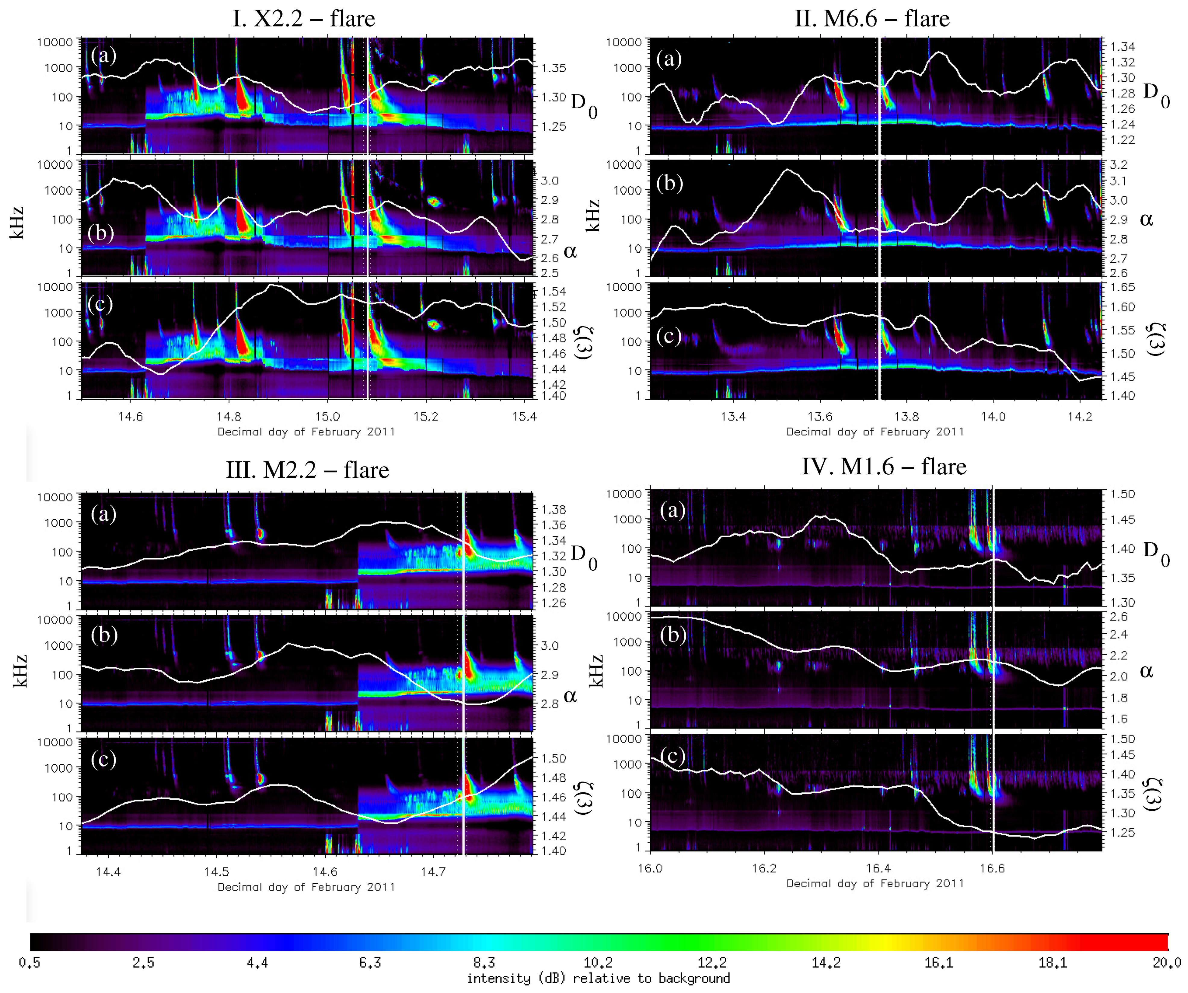
For the multiscale parameters, $D_0$, α and $\zeta \left(3\right)$, the respective parts of the time series are given in Figure 9. As in Figure 5, Figure 6 and Figure 7, we have complemented the time series with the co-temporal Wind/Waves spectra. As Figure 9 shows, clearly discernible Type II bursts are co-temporal with all major flares. This is evidence that flares are eruptive, which is confirmed by the launch locations and timing of the respective CMEs found in CME databases. The weakest Type II burst is associated with the M6.6 flare (column II in Figure 9) with the corresponding CME described as “poor” and “partial halo” in the LASCO/CME database.

The fractal dimension, $D_0$ (panel a in Figure 9), appears to be decreasing or having suffered a decrease a few hours prior to the flares. This is the case with flares X2.2, M2.2 and M1.6 (Figure 9Ia, Figure 9IIIa and and Figure 9IVa, respectively), while the M6.6 flare (Figure 9IIa) does not conform to this assessment. However, from this limited sample of flares, it is hard to discern a consistent preflare $D_0$-pattern as: (i) the X2.2 flare takes place after $D_0$ has reached a local minimum, hence in the course of a $D_0$-increase; (ii) the M2.2 flare occurs when $D_0$ evolves toward a local minimum, hence in the course of a $D_0$-decrease; and (iii) the M1.6 flare occurs in the course of a “step-like” decrease of $D_0$ that took place ∼5–7 h prior to the flare. In any case, a decrease in $D_0$ would imply a decrease of the boundary coverage of strong $B_z$-patterns in the AR. Magnetic-flux fragmentation and/or weakening of the $B_z$-patterns would give rise to such an effect.

The inertial-range scaling index, α, of the turbulent power spectrum (panel b in Figure 9) shows a rather more complicated pattern during flares. In particular, during the X2.2 flare (Figure 9Ib), α seems to be relatively insensitive with only the “long-term” decrease that took place after decimal day 14 (Figure 5c), appearing in the plot. A similar situation exists with the M1.6 flare (Figure 9IVb). In the case of the M6.6 flare (Figure 9IIb), α undergoes a significant decrease ∼3–5 h prior to the flare. During the M2.2 flare (Figure 9IIIb), finally, α is approximately at a local minimum. As with $D_0$, it is more physically meaningful to explain “long-term” changes of α, such as the increase and subsequent decrease after day 14, rather than short-term ones. The apparent lack of a consistent preflare pattern, at least for the present limited flare sample, on the other hand, makes it challenging to reach a consistent assessment about flare-related changes of α.

The intermittency scaling index, $\zeta \left(3\right)$ (panel c in Figure 9), seems to show the least consistency with flares. In the course of the X2.2 and M6.6 flares (Figure 9Ic and Figure 9IIc, respectively), $\zeta \left(3\right)$ appears rather insensitive, excluding a “step-like” increase that was completed $\sim 5$ h prior to the X2.2 flare. It is unclear whether this increase holds any relation to the flare. During the M2.2 flare (Figure 9IIIc), $\zeta \left(3\right)$ is clearly increasing, while it is clearly decreasing during the M1.6 flare (Figure 9IVc). More emphatically than in the case of $D_0$ and α, it is difficult to reach conclusions on possible flare-related $\zeta \left(3\right)$-changes in this study.

Figure 9. Details of the multiscale-parameter time series of Figure 5 corresponding to time intervals that include the occurrence of the four major flares of Table 1. Each set of stack plots (I, II, III, IV) corresponds to a given flare (X2.2, M6.6, M2.2 and M1.6, respectively). The onset time of each flare is indicated by the white lines. The time series of the fractal dimension, $D_0$, are shown in panels a. The time series of the turbulent scaling index α are shown in panels b, while the time series of the intermittency scaling index, $\zeta \left(3\right)$, are shown in panels c. Readings for multiscale parameters are given in the right ordinates. For additional information, each plot of a given stack includes the logarithmically-scaled co-temporal Wind/Waves frequency-time radio spectrum (readings in left ordinates).

Figure 9. Details of the multiscale-parameter time series of Figure 5 corresponding to time intervals that include the occurrence of the four major flares of Table 1. Each set of stack plots (I, II, III, IV) corresponds to a given flare (X2.2, M6.6, M2.2 and M1.6, respectively). The onset time of each flare is indicated by the white lines. The time series of the fractal dimension, $D_0$, are shown in panels a. The time series of the turbulent scaling index α are shown in panels b, while the time series of the intermittency scaling index, $\zeta \left(3\right)$, are shown in panels c. Readings for multiscale parameters are given in the right ordinates. For additional information, each plot of a given stack includes the logarithmically-scaled co-temporal Wind/Waves frequency-time radio spectrum (readings in left ordinates).

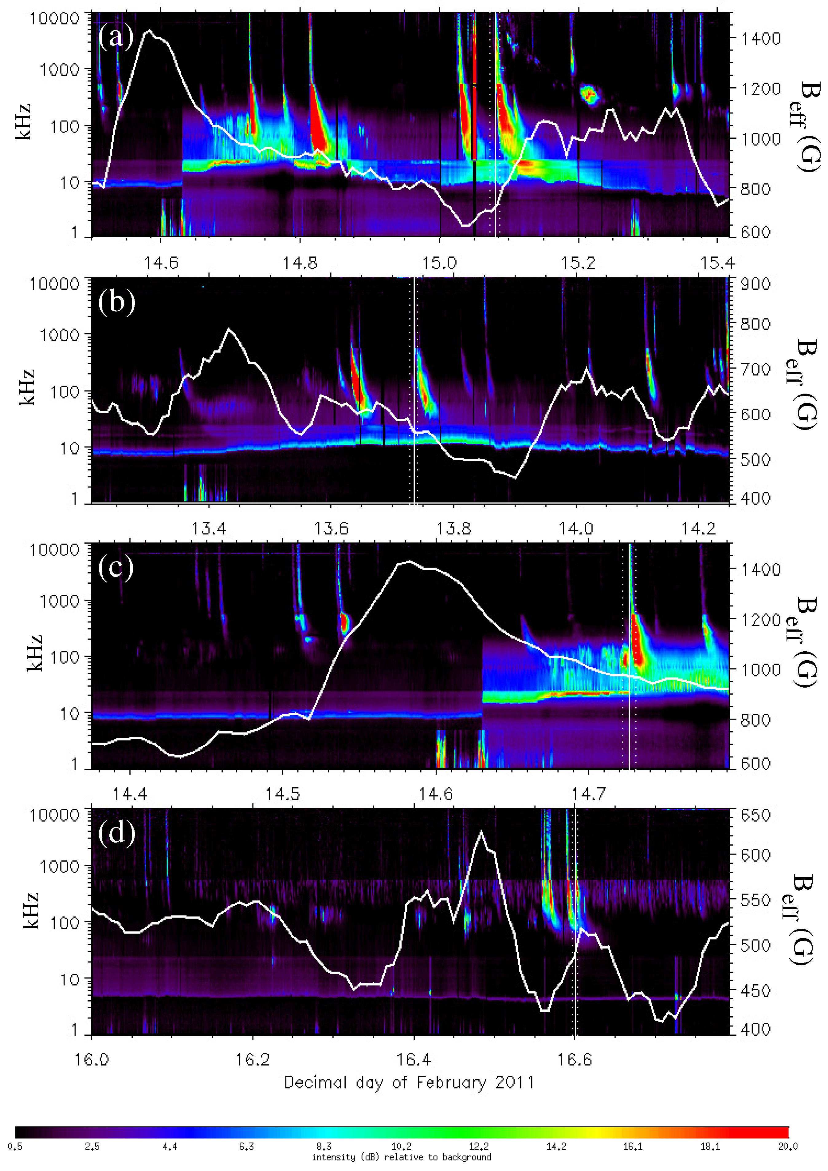
The same parts of the time series for the proxy parameter, $B_{eff}$, are shown in Figure 10. From it, one may argue on the following: while post-flare $B_{eff}$-behavior is mixed, there seems to exist a consistent, impulsive $B_{eff}$-increase prior to the flares, with the flares happening during the subsequent $B_{eff}$-decrease phase. For the X2.2 flare (Figure 10a), the impulse peaked ∼12 h prior to the flare onset. For the M6.6 flare (Figure 10b), the impulse peaked ∼7 h prior to the flare onset. For the M2.2 and M1.6 flares (Figure 10c and Figure 10d, respectively), the impulse peaked at ∼$3.5$ and ∼3 h prior to the flares, respectively. One might be tempted to comment on the shortening of the time delay between the preflare $B_{eff}$-peak and the flare itself for decreasing flare magnitudes. Such a claim, however, should be substantiated with a much larger flare sample and remains a topic for future studies. At present, we only report for the first time on this notable feature of the preflare $B_{eff}$-enhancement and emphasize the need to further investigate the effect for many more confined and eruptive flare events.

Figure 10. Details of the proxy parameter time series of Figure 6 corresponding to the same time intervals with those of Figure 9. The flares X2.2, M6.6, M2.2 and M1.6 are included in the time series of panels (a–d), respectively. The onset time of each flare is indicated by the thin white lines. Readings for the proxy parameter, $B_{eff}$, are given in the right ordinates. For additional information to each $B_{eff}$-plot, the logarithmically scaled co-temporal Wind/Waves frequency-time radio spectra (readings in the left ordinates) are included.

Figure 10. Details of the proxy parameter time series of Figure 6 corresponding to the same time intervals with those of Figure 9. The flares X2.2, M6.6, M2.2 and M1.6 are included in the time series of panels (a–d), respectively. The onset time of each flare is indicated by the thin white lines. Readings for the proxy parameter, $B_{eff}$, are given in the right ordinates. For additional information to each $B_{eff}$-plot, the logarithmically scaled co-temporal Wind/Waves frequency-time radio spectra (readings in the left ordinates) are included.

Figure 11. Details of the fundamental parameter time series of Figure 7 corresponding to the same time intervals with those of Figure 9. The relative magnetic helicity, $H_{mag}$, and the magnetic free energy, $E_c$, in each plot are shown with the green and orange curves, respectively (readings in the left ordinates). The flares X2.2, M6.6, M2.2 and M1.6 are included in the time series of plots a, b, c and d, respectively. The onset and end times of each flare are indicated by the dotted and dashed yellow lines, respectively, while flare peaks are indicated by the solid yellow line. For additional information on each plot, the logarithmically scaled co-temporal Wind/Waves frequency-time radio spectra (readings in the left ordinates) are included (adapted from [20]).

Figure 11. Details of the fundamental parameter time series of Figure 7 corresponding to the same time intervals with those of Figure 9. The relative magnetic helicity, $H_{mag}$, and the magnetic free energy, $E_c$, in each plot are shown with the green and orange curves, respectively (readings in the left ordinates). The flares X2.2, M6.6, M2.2 and M1.6 are included in the time series of plots a, b, c and d, respectively. The onset and end times of each flare are indicated by the dotted and dashed yellow lines, respectively, while flare peaks are indicated by the solid yellow line. For additional information on each plot, the logarithmically scaled co-temporal Wind/Waves frequency-time radio spectra (readings in the left ordinates) are included (adapted from [20]).

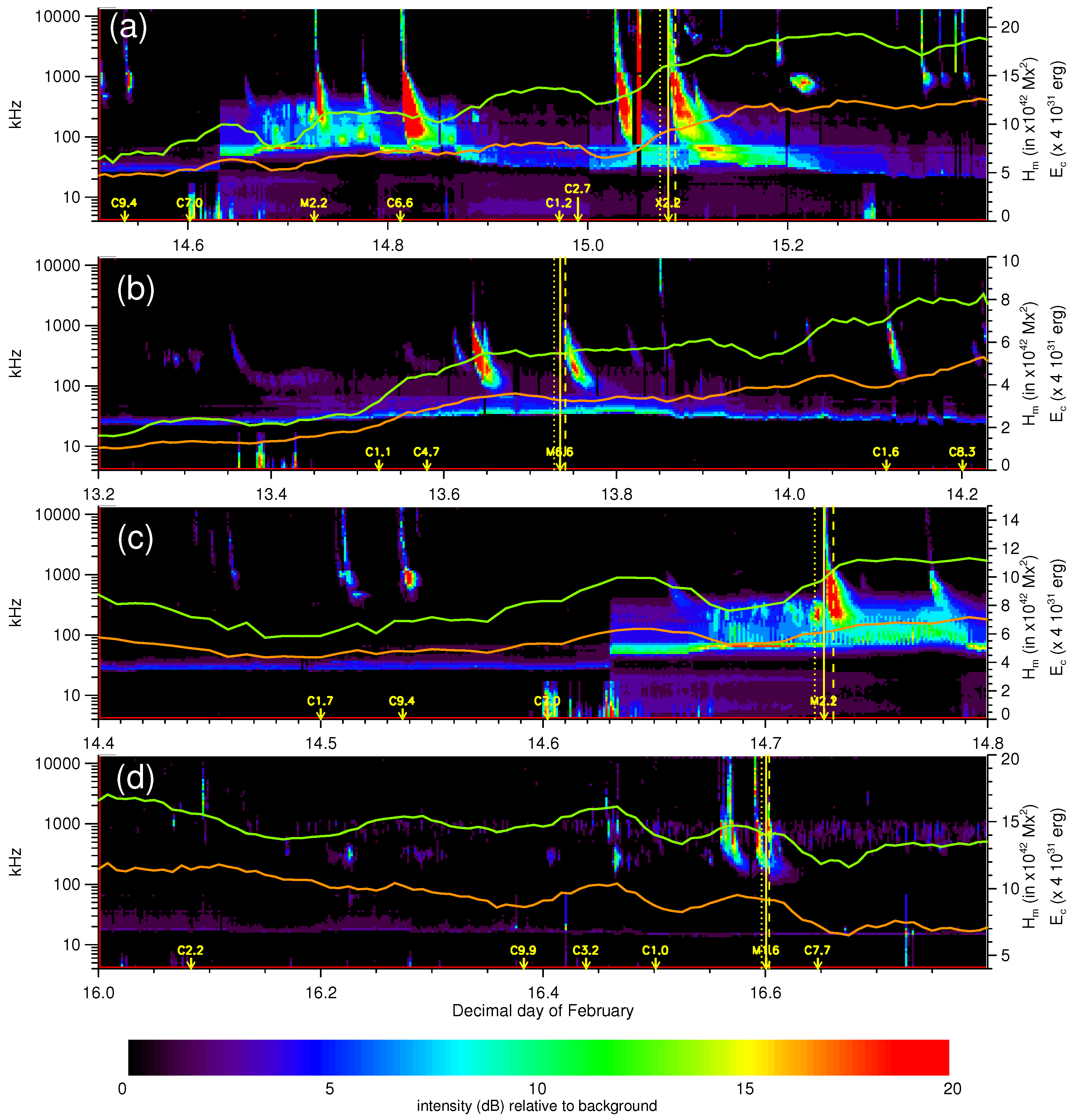
The same exercise for the fundamental physical parameters, $H_{mag}$ and $E_c$, was performed by [20] and is reproduced here in Figure 11. We notice a further distinct behavior compared to that of multiscale and proxy parameters. More specifically, the time series of $H_{mag}$ and $E_c$ are generally less erratic than those of multiscale and proxy parameters and tend to exhibit their “long-term” evolution over the five-day observing period. However, as originally explained in [20], a few hours before the flares, one notices transient decreases in both $H_{mag}$- and $E_c$-budgets that seem to be flare-related and, in fact, are compatible with an interpretation arguing that the CME progenitor starts ascending prior to the flare, with the flare being a natural consequence of the major perturbation caused by the CME initiation. This effect is clearly discernible for the X2.2, M2.2 and M1.6 flares (Figure 11a,c,d, respectively), and less so for the M6.6 flare (Figure 11b). Importantly, the decreases initiate much closer to the flare onset (typically ∼2 h) compared to the $B_{eff}$-enhancements discussed previously. As assessed in [20], this is understandable under the view that the dips relate to the initial CME ascension stages (it would be difficult to interpret this result in this respect if dips started, say, 10–12 h prior to the observed flare/CME event as in the case of $B_{eff}$). If we further recall that flares and CMEs, regardless of how intense, involve only a small fraction of the total accumulated $H_{mag}$- and $E_c$-budgets of the host active region [66], and that other effects (e.g., an overall active-region magnetic reorganization or the interaction with global solar magnetic fields [20]) are able to incur such and larger $H_{mag}$- and $E_c$-changes, then we realize that these budgets, while imperative for a physical and quantitative understanding of eruptive (and non-eruptive) active regions, may be of limited predictive value. This point was clearly made by [66], as well.

4.3. Direct Correlations between Parameters

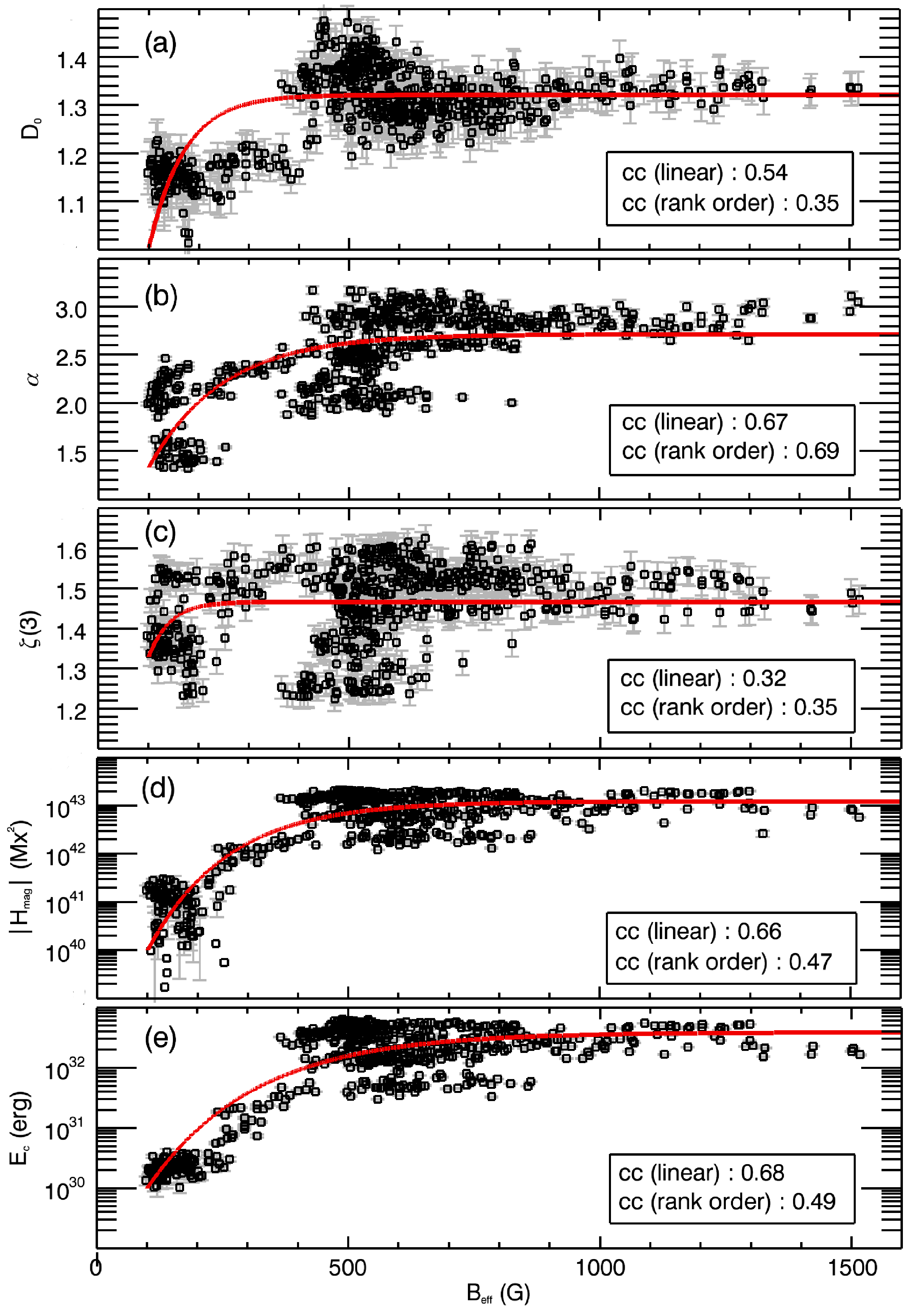
The final test we perform here is a direct correlation of parameter values for each of the 600 magnetograms of NOAA AR 11158. Since the proxy parameter, $B_{eff}$, appears as a potentially promising flare-prediction metric, we compare each of the other parameter values with $B_{eff}$-values. This exercise aims to: (i) determine which of the tested parameters correlate best with $B_{eff}$; and (ii) further quantify the apparently higher preflare behavior of $B_{eff}$-values compared to the other parameter values, at least for NOAA AR 11158. The results are shown in Figure 12.

In terms of scaling, Figure 12 suggests that $B_{eff}$ relates to all other parameters via a negative-exponential scaling relation of the form:

$$Y=A_0(1-e^{-A_1{B}_{eff}^{\prime }})$$

(9)

where $A_0$ and $A_1$ are fitting constants, $Y\equiv \{D_0,\alpha ,\zeta \left(3\right),|H_m|,E_c\}$ for Figure 12a–e, respectively, and $B_{eff}^{\prime }=B_{eff}-100$, with $B_{eff}^{\prime }>0$, since $B_{eff}>100$ G in all cases. Qualitatively, Equation (9) and Figure 12 suggest that while all parameters saturate at values $A_0$, $B_{eff}$ varies over a wide range at the same time. For $B_{eff}\in (500,\mathrm{1,500})$ G, that is, above the “background” $B_{eff}$-value of 500 G (Section 4.1), $D_0=1.32\pm 0.05$, $\alpha =2.70\pm 0.31$, $\zeta \left(3\right)=1.48\pm 0.09$, $|H_m|\in (0.7-1.1)\times {10}^{43}$ Mx${}^2$ and $E_c\in (1.8-2.9)\times {10}^{32}$ erg. These $B_{eff}$-values correspond to impulsive $B_{eff}$-enhancements that occur prior to major (>C-class) flares, as Figure 6 implies. We tentatively attribute this effect to the intuitive construction of $B_{eff}$ and perhaps other proxy parameters that emphasize active-region PILs; however, detailed additional investigation is required to fully understand this effect. Furthermore, the tendency of all multiscale parameters to reach saturation peaks at higher $B_{eff}$-values may imply a statistical tendency for active regions to be more likely to flare when their photospheric magnetic structures exhibit the highest intermittency and fractal dimension and/or when they exhibit the strongest departure from Kolmogorov and/or Kraichnan turbulence. This has been argued in earlier studies, as well, but as initially shown by [4] and further highlighted here, it has limited practical use toward flare prediction.

The inferred correlation coefficients in Figure 12 imply correlations varying between poor and moderately significant. In terms of multiscale parameters (Figure 12a–c), the best correlation is found between $B_{eff}$ and the scaling index, α (Figure 12b). A similar picture emerges when $B_{eff}$-values are correlated with fundamental-parameter values for $H_{mag}$ and $E_c$. Linear correlation coefficients for both correlations are moderately significant (∼$0.7$), implying that the proxy parameter, $B_{eff}$, scales only moderately in agreement with the relative magnetic helicity and the free magnetic energy. Rank-order coefficients imply even weaker correlations (∼$0.5$).

Figure 12. Direct correlation between the values of multiscale and fundamental parameters and the values of the proxy parameter, $B_{eff}$, for the 600 studied magnetograms of NOAA AR 11158. Shown are the correlations between $B_{eff}$ and (a) fractal dimension $D_0$; (b) scaling index α of the turbulent power spectrum; (c) multiscale intermittency index $\zeta \left(3\right)$; (d) $|H_{mag}|$ of the relative magnetic helicity; and (e) magnetic free energy $E_c$. The Pearson (linear) and Spearman (rank order) correlation coefficients are provided for each case. The negative-exponential curve at each plot (red) is the least-squared best-fit for the respective correlation.

Figure 12. Direct correlation between the values of multiscale and fundamental parameters and the values of the proxy parameter, $B_{eff}$, for the 600 studied magnetograms of NOAA AR 11158. Shown are the correlations between $B_{eff}$ and (a) fractal dimension $D_0$; (b) scaling index α of the turbulent power spectrum; (c) multiscale intermittency index $\zeta \left(3\right)$; (d) $|H_{mag}|$ of the relative magnetic helicity; and (e) magnetic free energy $E_c$. The Pearson (linear) and Spearman (rank order) correlation coefficients are provided for each case. The negative-exponential curve at each plot (red) is the least-squared best-fit for the respective correlation.

5. Summary and Conclusions

In recent years, numerous parameters implemented on solar (line-of-sight or vector) magnetograms have been proposed to hold the notable predictive ability of solar-flare occurrence. In a previous work [1], these parameters were segregated into different classes. For the multiscale class of parameters, including fractal and multifractal metrics, another study [4] showed and explained that (at least the tested) parameters are not efficient flare predictors. Per the interpretation given, the notion of multiscale behavior precisely inhibits the predictability of the system that exhibits it. Using multiscale parameters for flare prediction, therefore, seems to be of little meaning, in spite of the popularity of these parameters for the problem at hand.

The present study extends [4] by focusing on the detailed temporal behavior of multiscale parameters, but also of proxy and fundamental physical parameters, prior to and after major solar flares. As explained, proxy parameters rely mostly on magnetic morphology and are supposed to represent the fundamental physical parameters, namely the magnetic free energy and, per the findings of multiple works, the relative magnetic helicity. Evidently, a better predictive performance of fundamental physical quantities over their assumed proxies signals that the latter (sometimes constructed exclusively for this purpose) are not efficient flare predictors.

From the findings of Section 4, we conclude that: (1) intuitive proxy parameters seem more appropriate for an efficient flare prediction, even compared to fundamental physical parameters; (2) further work is needed to physically explain preflare impulses in proxy parameters ($B_{eff}$ in this case); and (3) the preflare proxy variability should be investigated in comprehensive statistical samples of eruptive and non-eruptive active regions.

Regarding our first conclusion, physical intuition seems instrumental for the construction of optimal proxies. Quantifying physical features, patterns or mechanisms that are long known to trigger flares (PILs, shear, impulsive flux emergence, sunspot rotation or all of them combined with optimal weighting) is probably our best course of action. Notice that this does not exclude, but rather it encourages, machine-learning (e.g., [67,68,69]) or combinatorial techniques that have been proposed as the only viable ones [70]. Per our preliminary results here, even a single, appropriate proxy may lead to advances of understanding. A word of caution for machine-learning methods is that regardless of sheer computing power, physical intuition of extracted patterns or features is necessary; otherwise, interpretation becomes challenging, and opportunities for further improvement are hindered. Regarding combinatorial methods, the combined parameters should not overlap, physically or numerically, but they should complement each other. Otherwise, increasingly complex, but overlapping parameter combinations may not necessarily lead to enhanced prediction efficiency.

The tested fundamental physical parameters show some preflare changes first detected and interpreted elsewhere [20], but at such short timescales that are not practical enough for prediction. This might be understood in view of the budgets of these parameters: with typical CME helicity contents of the order $(2-7)$×${10}^{42}$ Mx${}^2$ ([71,72]) and X-class flare energies ∼${10}^{32}$ erg [73], NOAA AR 11158 can give at least a few fast halo CMEs, several X-class flares and scores of M-/C-class flares at any given time. In this respect, other than short-term (and short-notice) $H_{mag}$- and $E_c$-changes that precede eruptive flares and reflect mainly the initial ascension of the CME progenitor [20], $H_{mag}$ and $E_c$ may not be expected to show conspicuous advance changes, even in the case of a X-class event.

Multiscale parameters, on the other hand, exhibit a preflare variability that cannot be unambiguously attributed to flares themselves, particularly given that the intensely eruptive NOAA AR 11158 and the very quiescent NOAA AR 11072 show not only similar multiscale-parameter values, but also similar morphologies of their respective time series (Figure 8).

Regarding our second conclusion, we plan to undertake detailed investigations to determine why $B_{eff}$ exhibits this distinctive behavior prior to major flares. This important question is posed on this study and remains to be answered physically. Inspection of the magnetic connectivity matrix in terms of morphology, size (number of flux tubes) and total flux content (connected flux), as well as detailed monitoring of the “open” flux in the various phases of these patterns are in order. It is important to underline at this point the difference between the apparent behavior of $B_{eff}$ and that of measurable magnetic-field variations ([18,74,75]) or Lorentz-force impulses ([76,77]) that have been interpreted as flare-related. These are clear transient or “permanent” changes, indeed, but they are detected in the course of flares and after them, not before them and at a practical time interval. As such, these signals cannot be used for flare forecasting, which is the core objective of the proxies introduced for this purpose.

Regarding our third conclusion, this study has revealed an additional result besides the predictive capability of proxy-parameter values, assessed from time series of cruder cadence: their detailed temporal profiles. Patterns, such as the ones found here for $B_{eff}$, may constitute grounds for improvement in predictive capability. Comprehensive statistics in fine-cadence time series will obviously be important in establishing this finding. In particular, one might employ a superposed epoch analysis (SEA) starting several (up to 24) hours prior to the flare to adequately cover the preflare phase. SEA results were discussed in [78], who showed that the sub-surface kinetic helicity of emerging host active regions, 2–3 days prior to flares, shows peaks that were increasingly conspicuous for increasing flare peak intensity (from the C- to X-class). We involved a SEA for the four major flares of Table 1, but, due to poor statistics (four major flares only), the resulting curves were dominated by noise. In any case, the need for incorporating the temporal profiles of flare-predictive metrics has been already spelled out in dedicated flare-prediction workshops [11]. Including the new information meaningfully will be a nontrivial exercise; the optimal course of action is unclear at the moment. The challenges of correctly incorporating the new information aside, obtaining solid, high-cadence statistics for this purpose seems only a matter of time if SDO/HMI data continue to flow uninterrupted for at least the scheduled SDO mission lifetime.

References and Notes

- Georgoulis, M.K. On Our Ability to Predict Major Solar Flares. In The Sun: New Challenges, Astrophysics and Space Science Proceedings; Obridko, V.N., Georgieva, K., Nagovitsyn, Y.A., Eds.; Springer-Verlag: Berlin/Heidelberg, Germany, 2012; pp. 93–104. [Google Scholar]
- Barnes, G.; Leka, K.D. Evaluating the performance of solar flare forecasting methods. Astrophys. J. 2008, 688, L107–L110. [Google Scholar] [CrossRef]
- Leka, K.D.; Barnes, G. Solar Flare Forecasting: A “State of the Field" Report for Researchers. In Proceedings of the AAS/SPD Meeting #44, Bozeman, MT, USA, 8–12 July 2013. Abstract # 100.82.
- Georgoulis, M.K. Are solar active regions with major flares more fractal, multifractal, or turbulent than others? Solar Phys. 2012, 276, 161–181. [Google Scholar] [CrossRef]
- Uritsky, V.M.; Paczuski, M.; Davila, J.M.; Jones, S.I. Coexistence of self-organized criticality and intermittent turbulence in the solar corona. Phys. Rev. Lett. 2007, 99, 025001. [Google Scholar] [CrossRef] [PubMed]
- Bak, P. How Nature Works: The Science of Self-Organized Criticality; Springer Verlag: New York, NY, USA, 1996. [Google Scholar]
- Nicolis, G.; Prigogine, I. Exploring Complexity. An Introduction; W. H. Freeman: New York, NY, USA, 1989. [Google Scholar]
- Uritsky, V.M.; Davila, J.M.; Ofman, L.; Coyner, A.J. Stochastic coupling of solar photosphere and corona. Astrophys. J. 2013, 769, 62:1–62:20. [Google Scholar] [CrossRef]
- Dimitropoulou, M.; Georgoulis, M.; Isliker, H.; Vlahos, L.; Anastasiadis, A.; Strintzi, D.; Moussas, X. The correlation of fractal structures in the photospheric and the coronal magnetic field. Astron. Astrophys. 2009, 505, 1245–1253. [Google Scholar] [CrossRef]
- Bloomfield, D.S.; Higgins, P.A.; McAteer, R.T.J.; Gallagher, P.T. Toward reliable benchmarking of solar flare forecasting methods. Astrophys. J. 2012, 747, L41:1–L41:7. [Google Scholar] [CrossRef]
- Leka, K.D.; Barnes, G.; The Flare Forecasting Comparison Group. The Second NWRA Flare-Forecasting Comparison Workshop: Methods Compared and Methodology. In Proceedings of the AAS/SPD Meeting #44, Bozeman, MT, USA, 8–12 July 2013. Abstract # 100.81.
- Georgoulis, M.K.; Tziotziou, K.; Raouafi, N.-E. Magnetic energy and helicity budgets in the active-region solar corona. II. Nonlinear force-free approximation. Astrophys. J. 2012, 759, 1:1–1:18. [Google Scholar] [CrossRef]
- Scherrer, P.H.; Schou, J.; Bush, R.I.; Kosovichev, A.G.; Bogart, R.S.; Hoeksema, J.T.; Liu, Y.; Duvall, T.L.; Zhao, J.; Title, A.M.; et al. The Helioseismic and Magnetic Imager (HMI) investigation for the Solar Dynamics Observatory (SDO). Solar Phys. 2012, 275, 207–227. [Google Scholar] [CrossRef]
- Pesnell, W.D.; Thompson, B.J.; Chamberlin, P.C. The Solar Dynamics Observatory (SDO). Solar Phys. 2012, 275, 3–15. [Google Scholar] [CrossRef]
- Lemen, J.R.; Title, A.M.; Akin, D.J.; Boerner, P.F.; Chou, C.; Drake, J.F.; Duncan, D.W.; Edwards, C.G.; Friedlaender, F.M.; Heyman, G.F.; et al. The Atmospheric Imaging Assembly (AIA) on the Solar Dynamics Observatory (SDO). Solar Phys. 2012, 275, 17–40. [Google Scholar] [CrossRef]
- Liu, C.; Deng, N.; Liu, R.; Lee, J.; Wiegelmann, T.; Jing, J.; Xu, Y.; Wang, S.; Wang, H. Rapid changes of photospheric magnetic field after tether-cutting reconnection and magnetic implosion. Astrophys. J. 2012, 745, L4:1–L4:7. [Google Scholar] [CrossRef]
- Schrijver, C.J.; Aulanier, G.; Title, A.M.; Pariat, E.; Delannée, C. The 2011 February 15 X2 flare, ribbons, coronal front, and mass ejection: Interpreting the three-dimensional views from the Solar Dynamics Observatory and STEREO guided by magnetohydrodynamic flux-rope modeling. Astrophys. J. 2011, 738, 167:1–167:23. [Google Scholar]
- Sun, X.; Hoeksema, J.T.; Liu, Y.; Wiegelmann, Th.; Hayashi, K.; Chen, Q.; Thalmann, J. Evolution of magnetic field and energy in a major eruptive active region based on SDO/HMI observation. Astrophys. J. 2012, 748, 77:1–77:15. [Google Scholar]
- Vemareddy, P.; Ambastha, A.; Maurya, R.A. On the role of rotating sunspots in the activity of solar active region NOAA 11158. Astrophys. J. 2012, 761, 60:1–60:13. [Google Scholar] [CrossRef]
- Tziotziou, K.; Georgoulis, M.K.; Liu, Y. Interpreting eruptive behavior in NOAA AR 11158 via the region’s magnetic energy and relative-helicity budgets. Astrophys. J. 2013, 772, 115:1–115:18. [Google Scholar] [CrossRef]
- Borrero, J.M.; Tomczyk, S.; Kubo, M.; Socas-Navarro, H.; Schou, J.; Couvidat, S.; Bogart, R. VFISV: Very fast inversion of the stokes vector for the helioseismic and magnetic imager. Solar Phys. 2011, 273, 267–293. [Google Scholar] [CrossRef]
- Leka, K.D.; Barnes, G.; Crouch, A.D.; Metcalf, T.R.; Gary, G.A.; Jing, J.; Liu, Y. Resolving the 180° ambiguity in solar vector magnetic field data: Evaluating the effects of noise, spatial resolution, and method assumptions. Solar Phys. 2009, 260, 83–108. [Google Scholar] [CrossRef]
- Georgoulis, M.K. Comment on “Resolving the 180° ambiguity in solar vector magnetic field data: evaluating the effects of noise, spatial resolution, and method assumptions”. Solar Phys. 2012, 276, 423–440. [Google Scholar] [CrossRef]
- Georgoulis, M.K. A New Technique for a routine azimuth disambiguation of solar vector magnetograms. Astrophys. J. 2005, 629, L69–L72. [Google Scholar] [CrossRef]
- Metcalf, Th.R.; Leka, K.D.; Barnes, G.; Lites, B.W.; Georgoulis, M.K.; Pevtsov, A.A.; Balasubramaniam, K.S.; Gary, G.A.; Jing, J.; Li, J.; et al. An overview of existing algorithms for resolving the 180° ambiguity in vector magnetic fields: Quantitative tests with synthetic data. Solar Phys. 2006, 237, 267–296. [Google Scholar] [CrossRef]
- Gary, G.A.; Hagyard, M.J. Transformation of vector magnetograms and the problems associated with the effects of perspective and the azimuthal ambiguity. Solar Phys. 1990, 126, 21–36. [Google Scholar] [CrossRef]
- Martens, P.C.H.; Attrill, G.D.R.; Davey, A.R.; Engell, A.; Farid, S.; Grigis, P.C.; Kasper, J.; Korreck, K.; Saar, S.H.; Savcheva, A.; et al. Computer vision for the Solar Dynamics Observatory (SDO). Solar Phys. 2012, 275, 79–113. [Google Scholar] [CrossRef]
- Hurlburt, N.; Cheung, M.; Schrijver, C.; Chang, L.; Freeland, S.; Green, S.; Heck, C.; Jaffey, A.; Kobashi, A.; Schiff, D.; et al. Heliophysics event knowledgebase for the Solar Dynamics Observatory (SDO) and beyond. Solar Phys. 2012, 275, 67–78. [Google Scholar] [CrossRef]
- Abramenko, V.I.; Yurchyshyn, V.B.; Wang, H.; Spirock, T.J.; Goode, P.R. Scaling behavior of structure functions of the longitudinal magnetic field in active regions on the sun. Astrophys. J. 2002, 577, 487–495. [Google Scholar] [CrossRef]
- Abramenko, V.I. Pre-flare changes in the turbulence regime for the photospheric magnetic field in a solar active region. Astron. Rep. 2003, 47, 151–160. [Google Scholar] [CrossRef]
- Abramenko, V.I.; Yurchyshyn, V.; Wang, H. Intermittency in the photosphere and corona above an active region. Astrophys. J. 2008, 681, 1669–1696. [Google Scholar] [CrossRef]
- McAteer, R.T.J.; Gallagher, P.T.; Ireland, J. Statistics of active region complexity: A large-scale fractal dimension survey. Astrophys. J. 2005, 631, 628–635. [Google Scholar] [CrossRef]
- Abramenko, V.I. Relationship between magnetic power spectrum and flare productivity in solar active regions. Astrophys. J. 2005, 629, 1141–1149. [Google Scholar] [CrossRef]
- Abramenko, V.I.; Yurchyshyn, V. Magnetic energy spectra in solar active regions. Astrophys. J. 2010, 720, 717–722. [Google Scholar] [CrossRef]
- Kolmogorov, A.N. Equations of turbulent motion in an incompressible fluid. Acad. Nauk USSR Ser. Fiz. 1942, 6, 56–58. [Google Scholar]
- Kraichnan, R.H. Inertial-range spectrum of hydromagnetic turbulence. Phys. Fluids 1965, 8, 1385–1387. [Google Scholar] [CrossRef]
- Frisch, U. Turbulence, the Legacy of A. N. Kolmogorov; Cambridge University Press: Cambridge, UK, 1995. [Google Scholar]
- Georgoulis, M.K. Turbulence in the solar atmosphere: Manifestations and diagnostics via solar image processing. Solar Phys. 2005, 228, 5–27. [Google Scholar] [CrossRef]
- McAteer, R.T.J.; Young, C.A.; Ireland, J.; Gallagher, P.T. The bursty nature of solar flare X-Ray emission. Astrophys. J. 2007, 662, 691–700. [Google Scholar] [CrossRef]
- McAteer, R.T.J. Private Communication, 2013.
- Schrijver, C.J. A characteristic magnetic field pattern associated with all major solar flares and its use in flare forecasting. Astrophys. J. 2007, 655, L117–L120. [Google Scholar] [CrossRef]
- Falconer, D.A.; Moore, R.L.; Gary, G.A.; Adams, M. The “Main Sequence" of explosive solar active regions: Discovery and interpretation. Astrophys. J. 2009, 700, L166–L169. [Google Scholar] [CrossRef]
- Mason, J.P.; Hoeksema, J.T. Testing automated solar flare forecasting with 13 years of michelson doppler imager magnetograms. Astrophys. J. 2012, 723, 634–640. [Google Scholar] [CrossRef]
- Schrijver, C.J. Driving major solar flares and eruptions: A review. Adv. Space Res. 2009, 43, 739–755. [Google Scholar] [CrossRef]
- Leka, K.D.; Barnes, G. Photospheric magnetic field properties of flaring versus flare-quiet active regions. I. Data, general approach, and sample results. Astrophys. J. 2003, 595, 1277–1295. [Google Scholar] [CrossRef]
- Georgoulis, M.K.; Rust, D.M. Quantitative forecasting of major solar flares. Astrophys. J. 2007, 661, L109–L112. [Google Scholar] [CrossRef]
- Bobra, M.G.; Georgoulis, M.K.; Hoeksema, J.T. Calculating Flaring Potential in Solar Active Regions Using SDO/HMI Vector Magnetic Field Data. In Proceedings of the First LWS/SDO Workshop, Squaw Valley, CA, USA, 1–5 May 2011.
- Higgins, P.A. Private Communication, 2013.
- Barnes, G.; Longcope, D.W.; Leka, K.D. Implementing a magnetic charge topology model for solar active regions. Astrophys. J. 2005, 629, 561–571. [Google Scholar] [CrossRef]
- Georgoulis, M.K.; Titov, V.S.; Mikić, Z. Non-neutralized electric current patterns in solar active regions: Origin of the shear-generating lorentz force. Astrophys. J. 2012, 761, 1:1–1:16. [Google Scholar] [CrossRef]
- Press, W.H.; Teukolsky, S.A.; Flannery, B.P.; Vetterling, W.T. Numerical Recipes in Fortran. The Art of Scientific Computing; Cambridge University Press: New York, NY, USA, 1992. [Google Scholar]
- Welsch, B.T.; Abbett, W.P.; de Rosa, M.L.; Fisher, G.H.; Georgoulis, M.K.; Kusano, K.; Longcope, D.W.; Ravindra, B.; Schuck, P.W. Tests and comparisons of velocity-inversion techniques. Astrophys. J. 2007, 670, 1434–1452. [Google Scholar] [CrossRef]
- De Rosa, M.L.; Schrijver, C.J.; Barnes, G.; Leka, K.D.; Lites, B.W.; Aschwanden, M.J.; Amari, T.; Canou, A.; McTiernan, J.M.; Régnier, S.; et al. A critical assessment of nonlinear force-free field modeling of the solar corona for active region 10953. Astrophys. J. 2009, 696, 1780–1791. [Google Scholar] [CrossRef]
- Metcalf, Th.R.; De Rosa, M.L.; Schrijver, C.J.; Barnes, G.; van Ballegooijen, A.A.; Wiegelmann, T.; Wheatland, M.S.; Valori, G.; McTtiernan, J.M. Nonlinear force-free modeling of coronal magnetic fields. II. Modeling a filament arcade and simulated chromospheric and photospheric vector fields. Solar Phys. 2008, 247, 269–299. [Google Scholar] [CrossRef]
- Schrijver, C.J.; De Rosa, M.L.; Metcalf, Th. R.; Liu, Y.; McTiernan, J.; Régnier, S.; Valori, G.; Wheatland, M.S.; Wiegelmann, T. Nonlinear force-free modeling of coronal magnetic fields Part I: A quantitative comparison of methods. Solar Phys. 2006, 235, 161–190. [Google Scholar] [CrossRef]
- McClymont, A.N.; Fisher, G.H. On the Mechanical Energy Available to Drive Solar Flares. In Yosemite Conference on Outstanding Problems in Solar Plasma Physics: Theory and Instrumentation; Waite, J.H., Burch, J.L., Moore, R.L., Eds.; AGU: Washington, DC, USA, 1989; pp. 219–225. [Google Scholar]
- Georgoulis, M.K.; LaBonte, B.J. Magnetic energy and helicity budgets in the active region solar corona. I. Linear force-free approximation. Astrophys. J. 2007, 671, 1034–1050. [Google Scholar] [CrossRef]
- Bougeret, J.-L.; Kaiser, M.L.; Kellogg, P.J.; Manning, R.; Goetz, K.; Monson, S.J.; Monge, N.; Friel, L.; Meetre, C.A.; Perche, C.; et al. Waves: The radio and plasma wave investigation on the wind spacecraft. Space Sci. Rev. 1995, 71, 231–263. [Google Scholar] [CrossRef]
- Klassen, A.; Aurass, H.; Mann, G.; Thompson, B. J. Catalogue of the 1997 SOHO-EIT coronal transient waves and associated type II radio burst spectra. Astron. Astrophys. Suppl. 2000, 141, 357–369. [Google Scholar] [CrossRef]
- Yashiro, S.; Gopalswamy, N.; Michalek, G.; St. Cyr, O.C.; Plunkett, S.P.; Rich, N.B.; Howard, R.A. A catalog of white light coronal mass ejections observed by the SOHO spacecraft. J. Geophys. Res. 2004, 109, A07105. [Google Scholar] [CrossRef]
- Olmedo, O.; Zhang, J.; Wechsler, H.; Poland, A.; Borne, K. Automatic detection and tracking of coronal mass ejections in coronagraph time series. Solar Phys. 2008, 248, 485–499. [Google Scholar] [CrossRef]
- Robbrecht, E.; Berghmans, D. Automated recognition of coronal mass ejections (CMEs) in near-real-time data. Astron. Astrophys. 2004, 425, 1097–1106. [Google Scholar] [CrossRef]
- Conlon, P.A.; McAteer, R.T.J.; Gallagher, P.T.; Fennell, L. Quantifying the evolving magnetic structure of active regions. Astrophys. J. 2010, 722, 577–585. [Google Scholar] [CrossRef]
- Howe, R.; Jain, K.; Bogart, R.S.; Haber, D.A.; Baldner, C.S. Two-dimensional helioseismic power, phase, and coherence spectra of solar dynamics observatory photospheric and chromospheric observables. Solar Phys. 2012, 281, 533–549. [Google Scholar] [CrossRef]
- Liu, Y.; Schuck, P.W. Magnetic energy and helicity in two emerging active regions in the sun. Astrophys. J. 2012, 761, 105:1–105:15. [Google Scholar] [CrossRef]
- Tziotziou, K.; Georgoulis, M.K.; Raouafi, N.-E. The magnetic energy-helicity diagram of solar active regions. Astrophys. J. 2012, 759, L4:1–L4:7. [Google Scholar] [CrossRef]
- Ahmed, O.W.; Qahwaji, R.; Colak, T.; Higgins, P.A.; Gallagher, P.T.; Bloomfield, D.S. Solar flare prediction using advanced feature extraction, machine learning, and feature selection. Solar Phys. 2013, 283, 157–175. [Google Scholar] [CrossRef]
- Song, H.; Tan, C.; Jing, J.; Wang, H.; Yurchyshyn, V.; Abramenko, V. Statistical assessment of photospheric magnetic features in imminent solar flare predictions. Solar Phys. 2009, 254, 101–125. [Google Scholar] [CrossRef]
- Yu, D.; Huang, X.; Hu, Q.; Zhou, R.; Wang, H.; Cui, Y. Short-term solar flare prediction using multiresolution predictors. Astrophys. J. 2010, 709, 321–326. [Google Scholar] [CrossRef]
- Leka, K.D.; Barnes, G. Photospheric magnetic field properties of flaring versus flare-quiet active regions. IV. A statistically significant sample. Astrophys. J. 2007, 656, 1173–1186. [Google Scholar] [CrossRef]
- DeVore, C.R. Magnetic helicity generation by solar differential rotation. Astrophys. J. 2000, 539, 944–953. [Google Scholar] [CrossRef]
- Georgoulis, M.K.; Rust, D.M.; Pevtsov, A.A.; Bernasconi, P.N.; Kuzanyan, K.M. Solar magnetic helicity injected into the heliosphere: Magnitude, balance, and periodicities over solar cycle 23. Astrophys. J. 2009, 705, L48–L52. [Google Scholar] [CrossRef]
- Hudson, H.S.; Fletcher, L.; Fisher, G.H.; Abbett, W.P.; Russell, A. Momentum distribution in solar flare processes. Solar Phys. 2012, 277, 77–88. [Google Scholar] [CrossRef]
- Sudol, J.J.; Harvey, J.W. Longitudinal magnetic field changes accompanying solar flares. Astrophys. J. 2005, 635, 647–658. [Google Scholar] [CrossRef]
- Wang, H.; Liu, C. Observational evidence of back reaction on the solar surface associated with coronal magnetic restructuring in solar eruptions. Astrophys. J. 2010, 716, L195–L199. [Google Scholar] [CrossRef]
- Fisher, G.H.; Bercik, D.J.; Welsch, B.T.; Hudson, H.S. Global forces in eruptive solar flares: The lorentz force acting on the solar atmosphere and the solar interior. Solar Phys. 2012, 277, 59–76. [Google Scholar] [CrossRef]
- Petrie, G.J.D. A spatio-temporal description of the abrupt changes in the photospheric magnetic and lorentz-force vectors during the 15 February 2011 X2.2 flare. Solar Phys. 2013, 287, 415–440. [Google Scholar] [CrossRef]
- Reinard, A.A.; Henthorn, J.; Komm, R.; Hill, F. Evidence that temporal changes in solar subsurface helicity precede active region flaring. Astrophys. J. 2010, 710, L121–L125. [Google Scholar] [CrossRef]
© 2013 by the author; licensee MDPI, Basel, Switzerland. This article is an open access article distributed under the terms and conditions of the Creative Commons Attribution license (http://creativecommons.org/licenses/by/3.0/).
Share and Cite
MDPI and ACS Style
Georgoulis, M.K. Toward an Efficient Prediction of Solar Flares: Which Parameters, and How? Entropy 2013, 15, 5022-5052. https://doi.org/10.3390/e15115022
AMA Style
Georgoulis MK. Toward an Efficient Prediction of Solar Flares: Which Parameters, and How? Entropy. 2013; 15(11):5022-5052. https://doi.org/10.3390/e15115022
Chicago/Turabian StyleGeorgoulis, Manolis K. 2013. "Toward an Efficient Prediction of Solar Flares: Which Parameters, and How?" Entropy 15, no. 11: 5022-5052. https://doi.org/10.3390/e15115022