Non–Parametric Estimation of Mutual Information through the Entropy of the Linkage

Abstract

A new, non–parametric and binless estimator for the mutual information of a d–dimensional random vector is proposed. First of all, an equation that links the mutual information to the entropy of a suitable random vector with uniformly distributed components is deduced. When $d=2$ this equation reduces to the well known connection between mutual information and entropy of the copula function associated to the original random variables. Hence, the problem of estimating the mutual information of the original random vector is reduced to the estimation of the entropy of a random vector obtained through a multidimensional transformation. The estimator we propose is a two–step method: first estimate the transformation and obtain the transformed sample, then estimate its entropy. The properties of the new estimator are discussed through simulation examples and its performances are compared to those of the best estimators in the literature. The precision of the estimator converges to values of the same order of magnitude of the best estimator tested. However, the new estimator is unbiased even for larger dimensions and smaller sample sizes, while the other tested estimators show a bias in these cases.

1. Introduction

The measure of multivariate association, that is, of the association between groups of components of a general d-dimensional random vector $X=(X_1,...,X_d)$, is a topic of increasing interest in a series of application contexts. Among the information measures, the mutual information, a special case of relative entropy or Kullback-Leibler distance [1], is a quantity that measures the mutual dependence between the variables considered. Unlike the measures of linear dependency between random variables, such as the correlation coefficient, the mutual information is particularly interesting as it is sensitive also to dependencies that are not codified in the covariance. Although this is one of the most popular dependency measures, it is only one of the many other existing ones, see for example [2].

The extension of mutual information to d–dimensional random vectors is not trivial [3,4,5]. Considering the distance between the joint distribution of the random vector and the joint distribution of the random vector with independent univariate components gives the so called total mutual information. However, in many instances, it is more interesting to study the distance between groups of components of the random vector, which are again multivariate random vectors of different dimensions. Hence the mutual information, in its general d–dimensional definition, is a distance of the joint distribution of the random vector to the joint distribution of groups of components considered independent from each other. We consider here this general framework with the aim of introducing a good estimator for the multivariate mutual information.

The problem of statistical estimation of mutual information has been considered by various authors. Optimized estimators that use adaptive bin sizes have been developed in [6,7]. A very good estimator based on k–nearest neighbor statistics is proposed in [8]. A computationally efficient modification of this method appeared recently in [9]. The estimation of mutual information sets in the broader context of the estimation of information–type measures such as entropy, Kullback–Leibler distance, divergence functionals, Rényi entropy. The k–nearest neighbor statistics are used to build an estimator for entropy in [10] and for the more general Rényi entropy in [11,12]. An overview of nonparametric entropy estimators can be found in [13]. For the case of discrete random variables, see for example [14]. A variational characterization of divergences allows the estimation of Kullback–Leibler divergence (and more generally any f–divergence) to turn into a convex optimization problem [15,16,17]. An interesting application of information–type quantities to devise a measure of statistical dispersion can be found in [18].

We propose here a new and simple estimator for the mutual information in its general multidimensional definition. To accomplish this aim, we first deduce an equation that links the mutual information between groups of components of a d-dimensional random vector to the entropy of the so called linkage function [19], that reduces to the copula function [20] in dimension $d=2$. In this way the problem of estimating mutual information is reduced to the estimation of the entropy of a suitably transformed sample of the same dimensions as the original random vector. This topic is hence closely related to the estimation of the Shannon entropy.

The structure of the paper is as follows: Notation and mathematical background are introduced in Section 2, where a brief survey on copula function and linkage function is also provided. In Section 3 we expose the method proposed to estimate the mutual information, providing also some details on the resulting algorithm and on the implementation care required. Section 4 contains some examples where the estimator is applied to simulated data and its performances are compared with some other estimators in literature. Conclusions are drawn in Section 5.

2. Notations and Mathematical Background

Given a $d-$dimensional random vector $X=(X_1,\cdots ,X_d)$, let us denote $F_{1,\cdots ,d}(x_1,\cdots ,x_d)=P(X_1\le x_1,\cdots ,X_d\le x_d)$, for $(x_1,\cdots ,x_d)\in {\mathbf{R}}^d$, the joint cumulative distribution function (c.d.f.) and $F_i\left(x\right)=P(X_i\le x)$, for $i=1,\cdots ,d$ and $x\in \mathbf{R}$, the marginal c.d.f. of the $i-$th component. When X is absolutely continuous, $f_{1,\cdots ,d}(x_1,\cdots ,x_d)$ for $(x_1,\cdots ,x_d)\in {\mathbf{R}}^d$ is the joint probability density function (p.d.f.) and $f_i\left(x\right)$ for $i=1,\cdots ,d$ and $x\in \mathbf{R}$ the corresponding marginal p.d.f. of the $i-$th component. Furthermore, $F_{i_1|i_2,\cdots ,i_l}\left(x_{i_1}\right|x_{i_2,\cdots ,x_{i_l}})$ and $f_{i_1|i_2,\cdots ,i_l}\left(x_{i_1}\right|x_{i_2},\cdots ,x_{i_l})$, where each $i_1,\cdots ,i_l$ assumes a different value ranging from 1 to d and $l=2,\cdots ,d$, denote respectively the conditional c.d.f. and the conditional p.d.f. of the variable $X_{i_1}$ with respect to the variables $X_{i_2},\cdots ,X_{i_d}$. For the sake of brevity, when $\alpha =({\alpha }_1,\cdots ,{\alpha }_n)$ is any multi–index of length n we use the following notation $F_{\alpha }\left(x_{\alpha }\right)=F_{{\alpha }_1,\cdots ,{\alpha }_n}(x_{{\alpha }_1},\cdots ,x_{{\alpha }_n)}$ denoting the c.d.f. of the random vector $X_{\alpha }=(X_{{\alpha }_1},\cdots ,X_{{\alpha }_n})$ and $f_{\alpha }\left(x_{\alpha }\right)=f_{{\alpha }_1,\cdots ,{\alpha }_n}(x_{{\alpha }_1},\cdots ,x_{{\alpha }_n)}$ denoting the p.d.f. of $X_{\alpha }$. Furthermore, when not necessary, we omit the argument of the functions, i.e., we may write $f_{\alpha }$ in spite of $f_{\alpha }\left(x_{\alpha }\right)$.

The mutual information (MI) of a 2-dimensional random vector $X=(X_1,X_2)$ is given by

$$MI(X_1,X_2)={\int }_{{\mathbf{R}}^2}{f}_{1,2}(x_1,x_2){log}_2\left[\frac{f_{1,2}(x_1,x_2)}{f_1\left(x_1\right)f_2\left(x_2\right)}\right]d{x}_{1}d{x}_2$$

(1)

If $X_1$ and $X_2$ are independent $MI(X_1,X_2)=0$.

The relative entropy (or Kullback-Leibler distance) D between the p.d.f.’s f and g is defined by

$$D\left(f∥g\right)={\int }_{{\mathbf{R}}^2}f(x_1,x_2)log\frac{f(x_1,x_2)}{g(x_1,x_2)}d{x}_{1}d{x}_2$$

(2)

Hence, MI can be interpreted as the Kullback-Leibler distance of the joint p.d.f. $f_{1,2}$ from the p.d.f. $f_1·f_2$ of a vector with independent components, i.e., it is a measure of the distance between $X=(X_1,X_2)$ and the random vector with the same marginal distributions but independent components.

The differential entropy of the absolutely continuous random vector $X=(X_1,\cdots ,X_d)$ is defined as

$$H(X_1,\cdots ,X_d)=-{\int }_{{\mathbf{R}}^d}{f}_{1,\cdots ,d}(x_1,\cdots ,x_d){log}_2{f}_{1,\cdots ,d}(x_1,\cdots ,x_d)d{x}_1\cdots d{x}_d$$

(3)

MI and entropy in the case $d=2$ are related through the well known equation [1]

$$MI(X_1,X_2)=H\left(X_1\right)+H\left(X_2\right)-H(X_1,X_2)$$

(4)

The generalization of MI to more than two random variables is not unique [3]. Indeed different definitions can be given according to different grouping of the components of the random vector $X=(X_1,\cdots ,X_d)$. More precisely, for any couple of multi-indices $(\alpha ,\beta )$ of dimensions h and k respectively, with $h+k=d$ and partitioning the set of indices $\left\{1,2,\cdots ,d\right\}$, the $MI(X_1,\cdots ,X_d)$ can be defined as the $MI(X_{\alpha },X_{\beta })$, where $X_{\alpha }=(X_{{\alpha }_1},\cdots ,X_{{\alpha }_h})$ and $X_{\beta }=(X_{{\beta }_1},\cdots ,X_{{\beta }_k})$. Therefore we have

$$\begin{array}{cc}MI(X_{\alpha },X_{\beta })& =\int f_{\alpha ,\beta }{log}_2\frac{f_{\alpha ,\beta }}{f_{\alpha }{f}_{\beta }}\hfill \\ & ={\int }_{{\mathbf{R}}^d}{f}_{1,\cdots ,d}(x_1,\cdots ,x_d){log}_2\left[\frac{f_{1,\cdots ,d}(x_1,\cdots ,x_d)}{f_{{\alpha }_1,\cdots ,{\alpha }_h}(x_{{\alpha }_1},\cdots ,x_{{\alpha }_h})f_{{\beta }_1,\cdots ,{\beta }_k}(x_{{\beta }_1},\cdots ,x_{{\beta }_k})}\right]d{x}_1\cdots d{x}_d\hfill \end{array}$$

(5)

More generally, for any n multi-indices $({\alpha }^1,\cdots ,{\alpha }^n)$ of dimensions $h_1,\cdots ,h_n$ respectively, such that $h_1+\cdots +h_n=d$ and partitioning the set of indices $\left\{1,2,\cdots ,d\right\}$ the following quantities

$$\begin{array}{cc}\hfill MI(X_{{\alpha }^1},\cdots ,X_{{\alpha }^n})& ={\int }_{{\mathbf{R}}^d}{f}_{{\alpha }^1,\cdots ,{\alpha }^n}{log}_2\frac{f_{{\alpha }^1,\cdots ,{\alpha }^n}}{f_{{\alpha }^1}\cdots f_{{\alpha }^n}}\hfill \\ & ={\int }_{{\mathbf{R}}^d}{f}_{1,\cdots ,d}(x_1,\cdots ,x_d)\times \hfill \\ & {log}_2\left[\frac{f_{1,\cdots ,d}(x_1,\cdots ,x_d)}{f_{{\alpha }_1^1,\cdots ,{\alpha }_{h_1}^1}(x_{{\alpha }_1^1},\cdots ,x_{{\alpha }_{h_1}^1})\cdots f_{{\alpha }_1^n,\cdots ,{\alpha }_{h_n}^n}(x_{{\alpha }_1^n},\cdots ,x_{{\alpha }_{h_n}^n})}\right]d{x}_1\cdots d{x}_d\hfill \end{array}$$

(6)

are all d–dimensional extensions of Equation (1). In the particular case $n=d$ where all the multi-indices have dimension 1, Equation (6) gives the so called total MI, a measure of the distance of the distribution of the given random vector to the one with the same marginal distributions but mutually independent components.

Equation (6) can be rewritten as

$$\begin{array}{cc}\hfill MI(X_{{\alpha }^1},\cdots ,X_{{\alpha }^n})& =\int f_{{\alpha }^1,\cdots ,{\alpha }^n}{log}_2{f}_{{\alpha }^1,\cdots ,{\alpha }^n}\hfill \\ & -\int f_{{\alpha }^1,\cdots ,{\alpha }^n}{log}_2{f}_{{\alpha }^1}-\cdots -\int f_{{\alpha }^1,\cdots ,{\alpha }^n}{log}_2{f}_{{\alpha }^n}\hfill \end{array}$$

(7)

and then, integrating each term, it is is easy to prove the following generalization to the d–dimensional case of Equation (4)

$$MI(X_{{\alpha }^1},\cdots ,X_{{\alpha }^n})=H\left(X_{{\alpha }^1}\right)+\cdots +H\left(X_{{\alpha }^n}\right)-H(X_1,\cdots ,X_d)$$

(8)

Another approach to the study of dependencies between random variables is given by copula functions (for example [20]). A $d-$dimensional copula (or $d-$copula) is a function $C:{[0,1]}^d\to [0,1]$ with the following properties:

(1)

for every $u=(u_1,\cdots ,u_d)\in {[0,1]}^d$, $C\left(u\right)=0$ if at least one coordinate is null and $C\left(u\right)=u_k$ if all coordinates are 1 except $u_k$;

(2)

for every $a=(a_1,\cdots ,a_d)$ and $b=(b_1,\cdots ,b_d)\in {[0,1]}^d$ such that $a\le b$, $V_C\left([a,b]\right)\ge 0$.

Here $V_C$ is the so called $C-$volume of $[a,b]$, i.e., the $n-$th order difference of C on $[a,b]$

$$V_C\left([a,b]\right)={\Delta }_{a_d}^{b_d}{\Delta }_{a_{d-1}}^{b_{d-1}}\cdots {\Delta }_{a_1}^{b_1}C\left(u\right)$$

(9)

where

$${\Delta }_{a_k}^{b_k}C\left(u\right)=C(u_1,\cdots ,u_{k-1},b_k,u_{k+1},\cdots ,h_d)-C(u_1,\cdots ,u_{k-1},a_k,u_{k+1},\cdots ,h_d)$$

(10)

Hence, a copula function is a non–decreasing function in each argument.

A central result in the theory of copulas is the so called Sklar’s theorem, see [20]. It captures the role that copulas play in the relationship between joint c.d.f.’s and their corresponding marginal univariate distributions. In particular it states that for any $d-$dimensional c.d.f. $F_{1,\cdots ,d}$ of the random vector $X=(X_1,\cdots ,X_d)$ there exists a $d-$copula C such that for all $x=(x_1,\cdots ,x_d)\in {\mathbf{R}}^d$

$$F_{1,\cdots ,d}(x_1,\cdots ,x_d)=C(F_1\left(x_1\right),\cdots ,F_d\left(x_d\right))$$

(11)

where $F_i$ are the univariate margins. If the margins are continuous, then the copula C is uniquely determined. Otherwise, C is uniquely determined over Ran$F_1\times \cdots \times$Ran$F_d$, where Ran$F_i$ is the range of the function $F_i$. Conversely, if C is a copula and $F_i$, $i=1,\cdots ,d$ are one-dimensional distribution functions, then the function $F_{1,\cdots ,d}(x_1,\cdots ,x_d)$ defined in Equation (11) is a d-dimensional distribution function with margins $F_i$, $i=1,\cdots ,d$.

In particular, a copula C can be interpreted as the joint c.d.f. of the random vector $U=(U_1,\cdots ,U_d)$, where each component is obtained through the transformation

$$U_i=F_i\left(X_i\right),i=1,\cdots ,d$$

(12)

Indeed

$$\begin{array}{ccc}\hfill P(U_1\le u_1,\cdots ,U_d\le u_d)& =& P(F_1\left(X_1\right)\le u_1,\cdots ,F_d\left(X_d\right)\le u_d)\hfill \\ & =& P(X_1\le F_1^{-1}\left(u_1\right),\cdots ,X_d\le F_d^{-1}\left(u_d\right))\hfill \\ & =& F_{1,\cdots ,d}(F_1^{-1}\left(u_1\right),\cdots ,F_d^{-1}\left(u_d\right))\hfill \\ \mathrm{(13)}& & =& C(u_1,\cdots ,u_d)\hfill \end{array}$$

Moreover, as each component is obtained with Equation (12), the univariate marginal distributions of the random vector U are all uniform on $[0,1]$. An important property that is tightly bound to MI is that copula functions are invariant under strictly increasing transformations of the margins, see [20].

If a copula C is differentiable, the joint p.d.f. of the random vector X can be written as

$$f_{1,\cdots ,d}(x_1,\cdots ,x_d)=\prod _{i=1}^d{f}_i\left(x_i\right)·c(F_1\left(x_1\right),\cdots ,F_d\left(x_d\right))$$

(14)

where

$$c(u_1,\cdots ,u_d)=\frac{{\partial }^d}{\partial u_1\cdots \partial u_d}C(u_1,\cdots ,u_d),u\in {[0,1]}^d$$

(15)

is the so called density of the copula C.

As illustrated in [21], it is not possible to use copula functions to handle multivariate distribution with given marginal distributions of general dimensions, since the only copula that is compatible with any assigned multidimensional marginal distributions is the independent one. To study dependencies between multidimensional random variables we resort to a generalization of copula notion. It relies on the use of the so-called linkage functions introduced in [19].

Let us consider the d-dimensional random vector X and any n multi-indices $({\alpha }^1,\cdots ,{\alpha }^n)$ of dimensions $(h_1,\cdots ,h_n)$ respectively, such that $h_1+\cdots +h_n=d$ and partitioning the set $\{1,2,\cdots ,d\}$. For $i=1,\cdots ,n$, let $F_{{\alpha }^i}$ be the $h_i$-dimensional c.d.f. of $X_{{\alpha }^i}=(X_{{\alpha }_1^i},\cdots ,X_{{\alpha }_{h_i}^i})$ and let $F_{{\alpha }^1,\cdots ,{\alpha }^n}$ be the joint c.d.f. of $X_{{\alpha }^1},\cdots ,X_{{\alpha }^n}$, which is of dimension d as the multi–indices are partitioning the set $\{1,2,\cdots ,d\}$.

Define the transformation ${\Psi }_{{\alpha }^i}:{\mathbf{R}}^{h_i}\to {[0,1]}^{h_i}$, $i=1,\cdots ,n$ as

$${\Psi }_{{\alpha }^i}(x_{{\alpha }_1^i},\cdots ,x_{{\alpha }_{h_i}^i})=(F_{{\alpha }_1^i}\left(x_{{\alpha }_1^i}\right),F_{{\alpha }_2^i|{\alpha }_1^i}\left(x_{{\alpha }_2^i}\right|x_{{\alpha }_1^i}),\cdots ,F_{{\alpha }_{h_i}^i|{\alpha }_1^i,\cdots ,{\alpha }_{h_i-1}^i}\left(x_{{\alpha }_{h_i}^i}\right|x_{{\alpha }_1^i},x_{{\alpha }_2^i},\cdots ,x_{{\alpha }_{h_i-1}^i}))$$

(16)

for all $x_{{\alpha }^i}$ in the range of $X_{{\alpha }^i}$.

Then the vectors

$$U_{{\alpha }^i}=(U_{{\alpha }_1^i},\cdots U_{{\alpha }_{h_i}^i})={\Psi }_{{\alpha }^i}(X_{{\alpha }_1^i},\cdots ,X_{{\alpha }_{h_i}^i})={\Psi }_{{\alpha }^i}\left(X_{{\alpha }^i}\right)$$

(17)

are $h_i$-dimensional vectors of independent uniform $[0,1]$ random variables, see [19].

The linkage function corresponding to the d-dimensional random vector $(X_{{\alpha }^1},\cdots ,X_{{\alpha }^n})$ is defined as the joint p.d.f. L of the vector

$$(U_{{\alpha }^1},\cdots ,U_{{\alpha }^n})=(U_{{\alpha }_1^1},\cdots ,U_{{\alpha }_{h_1}^1},\cdots ,U_{{\alpha }_1^n},\cdots ,U_{{\alpha }_{h_n}^n})=\left({\Psi }_{{\alpha }^1}\left(X_{{\alpha }^1}\right),\cdots ,{\Psi }_{{\alpha }^n}\left(X_{{\alpha }^n}\right)\right)$$

(18)

Notice that for $d=2$ the linkage function reduces to the copula function. Analogously to the two–dimensional case, linkages are invariant under strictly increasing functions, that is a d–dimensional function with components strictly increasing real univariate functions, see Theorem 3.4 in [19].

The information regarding the dependence properties between the multivariate components of the random vector $(X_{{\alpha }^1},\cdots ,X_{{\alpha }^n})$ is contained in the linkage function, that is independent from the marginal c.d.f.’s. Linkage functions can then be successfully employed when one is interested in studying the dependence properties between the random vectors $(X_{{\alpha }^1},\cdots ,X_{{\alpha }^n})$ disregarding their single components. On the other hand, linkage functions allow to study the interrelationships not only between all the components of a random vector, but also between given chosen sets of not overlapping random components of the vector. They contain the information regarding the dependence structure among such marginal vectors, while the dependence structure within the marginal vectors is not considered explicitly. It must be underlined that different multivariate c.d.f.’s $F_{{\alpha }^1,\cdots ,{\alpha }^n}$ can have the same linkage function but different marginal distributions.

In the next Section we will discuss the use of linkage functions for the computation of the MI between random vectors.

3. The Method

We propose here a method to estimate the MI of a d-dimensional random vector defined in Equation (6) by means of a random sample drawn from the corresponding d-dimensional joint distribution. We assume that neither the joint c.d.f. nor the marginal c.d.f.’s of the components of the random vector are known. The estimation approach proposed is then completely non parametric.

3.1. MI of a d–Dimensional Random Vector and Entropy of the Linkage

The method we are presenting is based on the equation between the MI of a d–dimensional random vector and its entropy deduced in the next theorem.

Theorem 1. Let $X=(X_1,\cdots ,X_d)$ be a d–dimensional random vector. For any n multi-indices $({\alpha }^1,\cdots ,{\alpha }^n)$ of dimensions $(h_1,\cdots ,h_n)$ respectively, such that $h_1+\cdots +h_n=d$ and partitioning the set of indices $\left\{1,2,\cdots ,d\right\}$, it holds

$$MI(X_{{\alpha }^1},\cdots ,X_{{\alpha }^n})=-H(U_{{\alpha }^1},\cdots ,U_{{\alpha }^n})$$

(19)

where $(U_{{\alpha }^1},\cdots ,U_{{\alpha }^n})=\left({\Psi }_{{\alpha }^1}\left(X_{{\alpha }^1}\right),\cdots ,{\Psi }_{{\alpha }^n}\left(X_{{\alpha }^n}\right)\right)$ and the function ${\Psi }_{{\alpha }^i},i=1,\cdots ,n$ are defined in Equation (16).

Proof. According to Equation (16) the random vector $(U_{{\alpha }^1},\cdots ,U_{{\alpha }^n})$ is obtained from $(X_1,\cdots ,X_d)$ by means of the following transformations:

$$\left\{\begin{array}{ccc}{U}_{{\alpha }_1^1}\hfill & =& F_{{\alpha }_1^1}\left(X_{{\alpha }_1^1}\right)\hfill \\ U_{{\alpha }_2^1}\hfill & =& F_{{\alpha }_2^1|{\alpha }_1^1}\left(X_{{\alpha }_2^1}\right|X_{{\alpha }_1^1})\hfill \\ & ⋮& \\ U_{{\alpha }_{h_1}^1}\hfill & =& F_{{\alpha }_{h_1}^1|{\alpha }_1^1,{\alpha }_2^1,\cdots ,{\alpha }_{h_1-1}^1}\left(X_{{\alpha }_{h_1}^1}\right|X_{{\alpha }_1^1},X_{{\alpha }_2^1},\cdots ,X_{{\alpha }_{h_1-1}^1})\hfill \\ U_{{\alpha }_1^2}\hfill & =& F_{{\alpha }_1^2}\left(X_{{\alpha }_1^2}\right)\hfill \\ U_{{\alpha }_2^2}\hfill & =& F_{{\alpha }_2^2|{\alpha }_1^2}\left(X_{{\alpha }_2^2}\right|X_{{\alpha }_1^2})\hfill \\ & ⋮& \\ U_{{\alpha }_1^n}\hfill & =& F_{{\alpha }_1^n}\left(X_{{\alpha }_1^n}\right)\hfill \\ & ⋮& \\ U_{{\alpha }_{h_n}^n}\hfill & =& F_{{\alpha }_{h_n}^n|{\alpha }_1^n,\cdots ,{\alpha }_{h_n-1}^n}\left(X_{{\alpha }_{h_n}^n}\right|X_{{\alpha }_{h_1}^n},\cdots ,X_{{\alpha }_{h_n-1}^n})\hfill \end{array}\right.$$

(20)

where the elements of the vector $(X_1,\cdots ,X_d)$ are grouped according to the multi–indices $({\alpha }^1,\cdots ,{\alpha }^n)$. The corresponding Jacobian matrix is given as follows

$$J=\left(\begin{array}{ccccccccccccc}\frac{\partial u_{{\alpha }_1^1}}{\partial x_{{\alpha }_1^1}}& 0& \cdots & 0& 0& 0& \cdots & 0& \cdots & 0& 0& \cdots & 0\\ \frac{\partial u_{{\alpha }_2^1}}{\partial x_{{\alpha }_1^1}}& \frac{\partial u_{{\alpha }_2^1}}{\partial x_{{\alpha }_2^1}}& \cdots & 0& 0& 0& \cdots & 0& \cdots & 0& 0& \cdots & 0\\ ⋮& ⋮& \ddots & ⋮& ⋮& ⋮& \ddots & ⋮& \cdots & ⋮& ⋮& \ddots & ⋮\\ \frac{\partial u_{{\alpha }_{h_1}^1}}{\partial x_{{\alpha }_1^1}}& \frac{\partial u_{{\alpha }_{h_1}^1}}{\partial x_{{\alpha }_2^1}}& \cdots & \frac{\partial u_{{\alpha }_{h_1}^1}}{\partial x_{{\alpha }_{h_1}^1}}& 0& 0& \cdots & 0& \cdots & 0& 0& \cdots & 0\\ 0& 0& \cdots & 0& \frac{\partial u_{{\alpha }_1^2}}{\partial x_{{\alpha }_1^2}}& 0& \cdots & 0& \cdots & 0& 0& \cdots & 0\\ 0& 0& \cdots & 0& \frac{\partial u_{{\alpha }_2^2}}{\partial x_{{\alpha }_1^2}}& \frac{\partial u_{{\alpha }_2^2}}{\partial x_{{\alpha }_2^2}}& \cdots & 0& \cdots & 0& 0& \cdots & 0\\ ⋮& ⋮& \ddots & ⋮& ⋮& ⋮& \ddots & ⋮& \cdots & ⋮& ⋮& \ddots & ⋮\\ 0& 0& \cdots & 0& \frac{\partial u_{{\alpha }_{h_2}^2}}{\partial x_{{\alpha }_1^2}}& \frac{\partial u_{{\alpha }_{h_2}^2}}{\partial x_{{\alpha }_2^2}}& \cdots & \frac{\partial u_{{\alpha }_{h_2}^2}}{\partial x_{{\alpha }_{h_2}^2}}& \cdots & 0& 0& \cdots & 0\\ ⋮& ⋮& ⋮& ⋮& ⋮& ⋮& ⋮& ⋮& \ddots & ⋮& ⋮& ⋮& ⋮\\ 0& 0& \cdots & 0& 0& 0& \cdots & 0& \cdots & \frac{\partial u_{{\alpha }_1^n}}{\partial x_{{\alpha }_1^n}}& 0& \cdots & 0\\ 0& 0& \cdots & 0& 0& 0& \cdots & 0& \cdots & \frac{\partial u_{{\alpha }_2^n}}{\partial x_{{\alpha }_1^n}}& \frac{\partial u_{{\alpha }_2^n}}{\partial x_{{\alpha }_2^n}}& \cdots & 0\\ ⋮& ⋮& \ddots & ⋮& ⋮& ⋮& \ddots & ⋮& \cdots & ⋮& ⋮& \ddots & ⋮\\ 0& 0& \cdots & 0& 0& 0& \cdots & 0& \cdots & \frac{\partial u_{{\alpha }_{h_n}^n}}{\partial x_{{\alpha }_1^n}}& \frac{\partial u_{{\alpha }_{h_n}^n}}{\partial x_{{\alpha }_2^n}}& \cdots & \frac{\partial u_{{\alpha }_{h_n}^n}}{\partial x_{{\alpha }_{h_n}^n}}\end{array}\right).$$

It is evident that the Jacobian matrix is a block diagonal matrix having as main diagonal blocks lower triangular matrices. Its determinant can be calculated as the product of the determinants of the main diagonal blocks, and hence

$$\left|J\right|=\frac{\partial u_{{\alpha }_1^1}}{\partial x_{{\alpha }_1^1}}\cdots \frac{\partial u_{{\alpha }_{h_1}^1}}{\partial x_{{\alpha }_{h_1}^1}}\frac{\partial u_{{\alpha }_1^2}}{\partial x_{{\alpha }_1^2}}\cdots \frac{\partial u_{{\alpha }_{h_2}^2}}{\partial x_{{\alpha }_{h_2}^2}}\frac{\partial u_{{\alpha }_1^n}}{\partial x_{{\alpha }_1^n}}\cdots \frac{\partial u_{{\alpha }_{h_n}^n}}{\partial x_{{\alpha }_{h_n}^n}}$$

(21)

Recalling the transformations given in Equation (20) we have

$$\begin{array}{ccc}\hfill \left|J\right|& =& \frac{\partial u_{{\alpha }_1^1}}{\partial x_{{\alpha }_1^1}}\cdots \frac{\partial u_{{\alpha }_{h_1}^1}}{\partial x_{{\alpha }_{h_1}^1}}\frac{\partial u_{{\alpha }_1^2}}{\partial x_{{\alpha }_1^2}}\cdots \frac{\partial u_{{\alpha }_{h_2}^2}}{\partial x_{{\alpha }_{h_2}^2}}\frac{\partial u_{{\alpha }_1^n}}{\partial x_{{\alpha }_1^n}}\cdots \frac{\partial u_{{\alpha }_{h_n}^n}}{\partial x_{{\alpha }_{h_n}^n}}\hfill \\ & =& \prod _{j=1}^n\left(\frac{\partial F_{{\alpha }_1^j}}{\partial x_{{\alpha }_1^j}}\prod _{i=2}^{h_j}\frac{\partial F_{{\alpha }_i^j|{\alpha }_1^j,\cdots ,{\alpha }_{i-1}^j}}{\partial x_{{\alpha }_i^j}}\right)\hfill \\ & =& \prod _{j=1}^n\left(f_{{\alpha }_1^j}\prod _{i=2}^{h_j}{f}_{{\alpha }_i^j|{\alpha }_1^j,\cdots ,{\alpha }_{i-1}^j}\right)\hfill \\ & =& \prod _{j=1}^n{f}_{{\alpha }_1^j,\cdots ,{\alpha }_{h_j}^j}\hfill \\ \mathrm{(22)}& & =& f_{{\alpha }^1}\cdots f_{{\alpha }^n}\hfill \end{array}$$

where the second to the last equality is obtained using iteratively the definition of conditional probability density function, i.e.,

$$f_{{\alpha }_1^j|{\alpha }_2^j}=\frac{f_{{\alpha }_1^j,{\alpha }_2^j}}{f_{{\alpha }_2^j}},f_{{\alpha }_3^j|{\alpha }_1^j,{\alpha }_2^j}=\frac{f_{{\alpha }_1^j,{\alpha }_2^j,{\alpha }_3^j}}{f_{{\alpha }_1^j,{\alpha }_2^j}},\cdots ,f_{{\alpha }_{h_j}^j|{\alpha }_1^j,\cdots ,{\alpha }_{h_j-1}^j}=\frac{f_{{\alpha }_1^j,\cdots ,{\alpha }_{h_j}^j}}{f_{{\alpha }_1^j,\cdots ,{\alpha }_{h_j-1}^j}}$$

As the random variables $(U_{{\alpha }^1},\cdots ,U_{{\alpha }^n})$ are the transformation of the vector $(X_1,\cdots ,X_d)$ given in Equation (20), their joint p.d.f. can be deduced as

$$f_{U_{{\alpha }^1},\cdots ,U_{{\alpha }^n}}(u_{{\alpha }^1},\cdots ,u_{{\alpha }^n})=\frac{f_{1,\cdots ,d}(x_1,\cdots ,x_d)}{\left|J\right|}$$

(23)

where $f_{1,\cdots ,d}$ is the joint p.d.f. of $(X_1,\cdots ,X_d)$ and $\left|J\right|$ is given in Equation (22). The last equation can be further simplified by renaming $(U_{{{\alpha }^1}_1},\cdots ,U_{{{\alpha }^1}_{h_1}},U_{{{\alpha }^2}_1},\cdots ,U_{{{\alpha }^2}_{h_2}},U_{{\alpha }_1^n,\cdots ,{\alpha }_{h_n}^n})=(U_1,\cdots ,U_d)$, and we get

$$f_{U_1,\cdots ,U_d}(u_1,\cdots ,u_d)=\frac{f_{1,\cdots ,d}(x_1,\cdots ,x_d)}{\left|J\right|}$$

(24)

From the d–dimensional definition of mutual information given in Equation (6) and applying the change of variables given in Equation (20) we have

$$\begin{array}{ccc}\hfill MI(X_{{\alpha }^1},\cdots ,X_{{\alpha }^n})& =& {\int }_{{\mathbf{R}}^d}{f}_{1,\cdots ,d}(x_1,\cdots ,x_d){log}_2\frac{f_{1,\cdots ,d}(x_1,\cdots ,x_d)}{f_{{\alpha }^1}\left(x_{{\alpha }^1}\right)\cdots f_{{\alpha }^n}\left(x_{{\alpha }^n}\right)}d{x}_1\cdots d{x}_d\hfill \\ \hfill & =& {\int }_{{\mathbf{R}}^d}{f}_{U_1,\cdots ,U_d}(u_1(x_1,\cdots ,x_d),\cdots ,u_d(x_1,\cdots ,x_d))\left|J\right|\hfill \\ \hfill & \times & {log}_2\left[f_{U_1,\cdots ,U_d}(u_1(x_1,\cdots ,x_d),\cdots ,u_d(x_1,\cdots ,x_d))\right]d{x}_1\cdots d{x}_d\hfill \\ \hfill & =& {\int }_{{[0,1]}^d}{f}_{U_1,\cdots ,U_d}(u_1,\cdots ,u_d){log}_2{f}_{U_1,\cdots ,U_d}(u_1,\cdots ,u_d)d{u}_1\cdots d{u}_d\hfill \end{array}$$

Just rewriting the last line of the previous equation using Equation (3), we get the thesis

$$MI(X_{{\alpha }^1},\cdots ,X_{{\alpha }^n})=-H(U_{{\alpha }^1},\cdots ,U_{{\alpha }^n})$$

(25)

□

Theorem 1 proves that the MI of a random vector can be computed without resorting to the marginal distributions, but rather transforming the components by means of Equation (20) into one-dimensional uniform $[0,1]$ random variables and then computing the Shannon entropy of the resulting vector.

Remark: Linkage functions do not change for monotone transformations. This property reflects the well know invariance property of MI under reparametrization.

In the particular case $d=2$ the definition of mutual information is simpler, see Equation (1) and the linkage functions reduce to the well known copula functions, as shown in the following

Corollary 1. The MI of the 2-dimensional random vector $X=(X_1,X_2)$ can be obtained as

$$MI(X_1,X_2)=-H\left(U_1,U_2\right)$$

(26)

where $U_1=F_1\left(X_1\right)$ and $U_2=F_2\left(X_2\right)$.

Proof. For $d=2$ the only non trivial choice of multi–indices partitioning the set $\{1,2\}$ is ${\alpha }^1=1$ and ${\alpha }^2=2$, hence $h_1=1$ and $h_2=1$. The transformations given in Equation (20) reduce to Equation (12) for $d=2$

$$\left\{\begin{array}{ccc}{U}_1\hfill & =& F_1\left(X_1\right)\hfill \\ U_2\hfill & =& F_2\left(X_2\right)\hfill \end{array}\right.$$

(27)

Let us notice that the joint c.d.f. of the couple $(U_1,U_2)$ is the copula function, see Equation (13). Hence their p.d.f. is obtained as

$$f_{1,2}(x_1,x_2)=\frac{{\partial }^2}{\partial x_1\partial x_2}C(F_1\left(x_1\right),F_2\left(x_2\right))=c(F_1\left(x_1\right),F_2\left(x_2\right))f_1\left(x_1\right)f_2\left(x_2\right)$$

(28)

where $c(u_1,u_2)$ is the copula density defined in Equation (15). In this special case Equation (22) reduces to

$$\left|J\right|=f_1\left(x_1\right)f_2\left(x_2\right)$$

(29)

and the definition given in Equation (1) can be rewritten as

$$\begin{array}{ccc}\hfill MI(X_1,X_2)& =& {\int }_{{\mathbf{R}}^2}{f}_1\left(x_1\right)f_2\left(x_2\right)c\left(F_1\left(x_1\right),F_2\left(x_2\right)\right){log}_{2}c\left(F_1\left(x_1\right),F_2\left(x_2\right)\right)d{x}_{1}d{x}_2\hfill \\ & =& {\int }_{{[0,1]}^2}c(u_1,u_2){log}_{2}c(u_1,u_2)d{u}_{1}d{u}_2\hfill \\ & =& -H\left(U_1,U_2\right)\hfill \end{array}$$

Hence, the MI between two one-dimensional random variables can be computed without resorting to the marginal distributions of the two variables, but transforming them into the corresponding one-dimensional uniform $[0,1]$ variables according to Equation (12) and then computing their Shannon entropy. Equation (26) can be equivalently rewritten as

$$MI(X_1,X_2)=E_C\left[{log}_{2}c(U_1,U_2)\right]$$

(30)

where $E_C$ denotes the expectation with respect to the copula distribution. Note that the result concerning $d=2$ has already been obtained in [22,23] and one of the more impactful studies that exploits this equality is [24].

Example. In the particular case where $X=(X_1,X_2,X_3)$ and the multi–indices are chosen such that $X_{{\alpha }^1}=X_1$ and $X_{{\alpha }^2}=(X_2,X_3)$ we have

$$MI(X_{{\alpha }^1},X_{{\alpha }^2})=-H(U_1,U_2,U_3)$$

(31)

where

$$\left\{\begin{array}{c}{U}_1=F_1\left(X_1\right)\hfill \\ U_2=F_2\left(X_2\right)\hfill \\ U_3=F_{3|2}\left(X_3\right|X_2)\hfill \end{array}\right.$$

(32)

Let us remark that the choice of the multi–indices grouping the elements of the random vector X uniquely determines the transformation given in Equation (32) required to properly get the random vector $U_1,U_2,U_e$ such that Equation (31) holds true. Different choices of multi–indices give different transformations and different random vectors U’s.

3.2. The Estimation Procedure

Let $(X^1,\cdots ,X^N)$ be a random sample of size N drawn from the multivariate distribution $F_{1,\cdots ,d}$ of the random vector X. Using Theorem 1, we propose here a method to estimate the mutual information of the random vector X in its general definition, i.e., the $MI(X_{{\alpha }^1},\cdots ,X_{{\alpha }^n})$ for any n multi-indices $({\alpha }^1,\cdots ,{\alpha }^n)$ of dimensions $(h_1,\cdots ,h_n)$ respectively, such that $h_1+\cdots +h_n=d$ and partitioning the set $1,2,\cdots ,d$.

Let us proceed as follows:

• estimate the conditional c.d.f.’s in Equation (20). Denote these functions as ${\widehat{\Psi }}_{{\alpha }^i}=({\widehat{F}}_{{\alpha }_1^i},{\widehat{F}}_{{\alpha }_2^i|{\alpha }_2^i},\cdots ,{\widehat{F}}_{{\alpha }_{h_i}^i|{\alpha }_{h_i-1}^i})$, for $i=1,\cdots ,n$;
• for $k=1,\cdots ,N$ calculate $U^k=(U_{{\alpha }^1}^k,\cdots ,U_{{\alpha }^n}^k)$, where $U_{{\alpha }^i}^k=({\widehat{\Psi }}_{{\alpha }^1}\left(X_{{\alpha }^1}^k\right),\cdots ,{\widehat{\Psi }}_{{\alpha }^n}\left(X_{{\alpha }^n}^k\right))$, for $i=1,\cdots ,n$;
• estimate the $MI(X_{{\alpha }^1},\cdots ,X_{{\alpha }^n})$ as the Shannon entropy in Equation (19) of the transformed sample $(U^1,\cdots ,U^N)$.

For the particular case when $d=2$ the procedure becomes the following:

• estimate the c.d.f.’s in Equation (27). Denote the estimated functions as $({\widehat{F}}_1,{\widehat{F}}_2)$;
• calculate $U^k=({\widehat{F}}_1\left(X_1^k\right),{\widehat{F}}_2\left(X_2^k\right))$, for $k=1,\cdots ,N$;
• estimate $MI(X_1,X_2)$ as the Shannon entropy in Equation (26) of the transformed sample $(U^1,\cdots ,U^N)$.

Let us now enter the details of the above illustrated procedure. The performances of the proposed method strongly depend on the estimators used for the c.d.f.’s and conditional c.d.f.’s at step 1 and the entropy at step 3 of the above proposed algorithm.

Step 1 of the procedure: estimating c.d.f’s. Let us compare the performances of the estimation algorithm for three different choices of the estimator for the c.d.f.’s, namely the empirical distribution function, the kernel density estimator and the k–nearest neighbor density estimator.

The most natural estimator for the c.d.f is the empirical distribution function, that for $(X^1,\cdots ,X^N)$ a univariate random sample of size N is defined as

$${\widehat{F}}_N\left(t\right)=\frac{1}{N}\sum _{i=1}^N{\mathbf{1}}_{(-\infty ,t]}\left(X^i\right)$$

(33)

Despite its good asymptotic properties, the empirical distribution function exhibits a slow rate of convergence, see for example [25] where it is shown that the empirical distribution function is a deficient estimator with respect to a certain class of kernel type estimators. It could be then necessary to resort to more reliable techniques to estimate the c.d.f.’s.

As suggested in [25], we could consider kernel–based density estimators, both to estimate the univariate c.d.f.’s and the conditional c.d.f.’s, where the conditioning random variable could be multivariate, see Equation (20). Let us recall that, given $X^1,\cdots ,X^N$ a random sample of size N drawn from a law with p.d.f. f, the univariate kernel density estimator for f is obtained as

$${\widehat{f}}_{ker}\left(x\right)=\frac{1}{Nh}\sum _{i=1}^{N}K\left(\frac{x-X^i}{h}\right)$$

(34)

where K is a suitable function called kernel, that is required to be a normalized probability density, and h is a positive number called the bandwidth, see [26,27]. One of the most commonly used kernel is the Gaussian kernel

$${\widehat{f}}_{ker}\left(x\right)=\frac{1}{Nh}\sum _{i=1}^N\frac{1}{\sqrt{2\pi }}exp\left(-\frac{{(x-X^i)}^2}{2h^2}\right)$$

(35)

However, depending on the properties of the density to be estimated, it can be convenient to consider different kernels. For example the rectangular kernel and the Gamma kernel can be recommended to estimate the uniform and the exponential distributions respectively. The bandwidth h has to be chosen carefully as too small values can give rise to spurious fine structures of the estimate, while too large values can hide all the details in the estimated density curve. The choice of a possible optimal bandwidth usually falls on the one that minimizes the mean integrated square error. When it is assumed that the underlying distribution is Gaussian, the optimal bandwidth $h_{opt}$ is given by

$$h_{opt}={\left(\frac{4}{3N}\right)}^{\frac{1}{5}}\sigma \cong 1.06\sigma N^{-\frac{1}{5}}$$

(36)

where σ denotes the standard deviation of the sample values, see [26]. Let us remark that having no parametric hypothesis on the distribution of the random vector considered, in our method the choice of the kernel function and of the bandwidth should be made by visual inspection of the histograms of the involved distributions.

A third choice to estimate the c.d.f.’s could rely on the nearest neighbor density estimator, see [27,28]. Let us recall that, given $X^1,\cdots ,X^N$ a random sample of size N drawn from a law with p.d.f. f, the nearest neighbor density estimator for f is obtained as

$${\widehat{f}}_{knn}\left(x\right)=\frac{k}{NV}$$

(37)

where k is fixed and V is the volume of the sphere that contains precisely k data points, the $k-$nearest to x. A possible generalization of the nearest neighbor estimator provides an estimator of the kernel type again, as in Equation (34) but with bandwidth h equal to the distance between x and its $k-$nearest neighbor. As actually the generalized nearest neighbor is a kernel estimator with a suitable choice of the bandwidth parameter, we are calling nearest neighbor density estimator only the simple one given in Equation (37).

For the estimation of conditional densities, some papers propose methods improving the naive kernel estimator obtained as the ratio of the multidimensional kernel estimators for the joint p.d.f. and the joint p.d.f. of the conditioning variables, see [29,30,31]. In this paper we use the estimator proposed in [30] and successively improved in [31], based on a locally polynomial regression.

The performances of our estimator for the three different choices of c.d.f.’s estimations are compared in Figure 1. The samples are drawn from a bivariate gaussian distribution with standard marginal distributions and correlation coefficient $\rho =0.9$ for different sample sizes N. The accuracy of the estimation increases with increasing sample size, but the best performance is definitely obtained with the kernel density estimator (black).

Figure 1. 95% confidence intervals of the estimated MI of a bivariate gaussian distribution as the sample size N increases. True value of MI = 1.1979 bits. Cumulative distribution functions are estimated by the empirical distribution function given in Equation (33) (blue), the kernel density estimator given in Equation (34) (black) and the $k-$nearest neighbor density estimator given in Equation (37) (red).

Figure 1. 95% confidence intervals of the estimated MI of a bivariate gaussian distribution as the sample size N increases. True value of MI = 1.1979 bits. Cumulative distribution functions are estimated by the empirical distribution function given in Equation (33) (blue), the kernel density estimator given in Equation (34) (black) and the $k-$nearest neighbor density estimator given in Equation (37) (red).

Step 3 of the procedure: estimating entropy. The second important point that requires some care, is the estimation of the differential entropy of the transformed sample at step 3 of our method. Also in this case the estimation can be performed using a kernel type estimator or a nearest neighbor one.

The unbinned nearest-neighbor method proposed in [10,32] seems to have good properties. It is based on nearest–neighbor Euclidean distances and it has been shown to be asymptotically unbiased and consistent, provided that the underlying p.d.f. obeys certain conditions that control the convergence of the integrals for the differential entropy, see [10]. Given a random sample of size N from the $d-$dimensional random vector $X=(X_1,\cdots ,X_d)$, the estimator proposed for the differential entropy is given by

$${\widehat{H}}_{knn}=\frac{d}{N}\sum _{j=1}^N{log}_2\left({\lambda }_j\right)+{log}_2\left[\frac{S_d(N-1)}{d}\right]+\frac{\gamma }{ln\left(2\right)}$$

(38)

where $\gamma =-{\int }_0^{\infty }{e}^{-v}lnvdv\cong 0.5772156649$ is the Euler-Mascheroni constant, ${\lambda }_j$ is the Euclidean distance of each sample point to its nearest neighbor and

$$S_d=\frac{d{\pi }^{d/2}}{\Gamma (\frac{d}{2}+1)}$$

with Γ the gamma function is the area of a unit d-dimensional spherical surface (for example $S_1=2,$ $S_2=2\pi ,S_3=4\pi ,\cdots )$.

Another choice could be an estimator of the kernel type, see [13]. The so called resubstitution estimate proposed in [13] is of the form

$${\widehat{H}}_{ker}=-\frac{1}{N}\sum _{i=1}^{N}log{\widehat{f}}_{ker}\left(X_i\right)$$

(39)

where ${\widehat{f}}_{ker}$ is a kernel density estimate.

Figure 2. 95% confidence intervals of the estimated MI of a bivariate gaussian distribution as the sample size N increases. True value of MI = 1.1979 bits. Entropy is estimated by the $k-$ nearest neighbor given in Equation (38) (black) and the kernel type entropy estimator given in Equation (39) (green).

Figure 2. 95% confidence intervals of the estimated MI of a bivariate gaussian distribution as the sample size N increases. True value of MI = 1.1979 bits. Entropy is estimated by the $k-$ nearest neighbor given in Equation (38) (black) and the kernel type entropy estimator given in Equation (39) (green).

The performances of our estimator for the two different choices of entropy estimators are compared in Figure 2. Again, the samples are drawn from a bivariate gaussian distribution with standard marginal distributions and correlation coefficient $\rho =0.9$ for different sample sizes N. The best performance is definitely obtained with the $k-$ nearest neighbor entropy estimator (black).

Hence we come to the conclusion that the best results are obtained using a kernel type density estimator at the step 1 of the method and with a k–nearest neighbor entropy estimator at the step 3 of the method. This is the chosen procedure for the examples proposed in the next Section.

4. Examples and Simulation Results

In this Section we show the results obtained with the estimator proposed in Section 3. The examples cover the cases $d=2,3,4$. We choose cases for which the MI can be computed either in a closed form expression or numerically, so that we can easily compare our results with the exact ones.

Several methods have been already proposed in the literature to estimate the MI between multivariate random vectors from sample data. One of the most efficient seems to be the binless method exposed in [8], based on estimates from k–nearest neighbor statistics. We refer from now on to this method as “KSG” from the names of the authors. On the other hand, a straightforward way to estimate MI could be to estimate separately the entropy terms in Equation (8) by means of a suitable estimator as the one proposed in [10,32] and sum them up. Let us notice that this procedure is not recommended as the errors made in the individual estimates of each entropy term would presumably not cancel. We refer to this methodology as the “plain entropy” method. The results obtained with our estimator are here compared both to the KSG and to the “plain entropy”.

As mutual information is a particular case of Kullback–Leibler divergence, we could use the estimators proposed in [15,17]. However let us remark that our estimator is based on one single sample of size N drawn from $f_{1,\cdots ,d}$, the multivariate joint law of the random vector $(X_1,\cdots ,X_d)$. On the other side, the estimators proposed in [15,17] and adapted to the case of mutual information are based on two samples: one drawn from the multivariate joint law and the other from $f_{{\alpha }^1}\cdots f_{{\alpha }^n}$, the product of the n marginal laws. We could build the missing sample from the given one, but it is not obvious that the estimators will keep their good properties. Indeed in our setting the samples are no more independent as some resampling procedure should be devised to make the method suitable for our particular case. From a preliminary numerical study it seems that the performances of the estimators proposed in [15,17] are not comparable to the performances of our estimator. Hence we skip this comparison.

The examples illustrated in the next two Subsections are chosen to test our approach on distributions that could be troublesome for our approach. Following the discussion introduced in the previous Section, the delicate point of the method is the estimation of the (conditional) cumulative distribution functions in Equation (20). Hence we consider an example where the density to be estimated has bounded support as for the Uniform r.v. (Example 2) and an example where the density is positive valued and with an early steep peak as for the Exponential r.v. (Example 3). To address the problem of tails in estimation of information–theoretic quantities, we present two examples of heavy-tailed distributions: the lognormal (Example 4) and the Levy (Example 5). Note that the lognormal distribution is heavy tailed but with finite all order moments, while the Levy is an alpha–stable distribution with power law tail probability and no finite moments.

We rely on simulated data, while we reserve to a future work the application of the estimator to data coming from real experiments. For each example we perform $m=100$ simulation batches of the random vectors involved for each of the following sample sizes $N=100,500,1000,2000,3000$.

4.1. Two-Dimensional Vectors

Let us consider the following five cases of two-dimensional random vectors $X=(X_1,X_2)$.

• Example 1. Let $X=(X_1,X_2)$ be a gaussian random vector with standard normal components and correlation coefficient $\rho =0.9$. Denoting as σ the covariance matrix of X, the MI between $X_1$ and $X_2$ is given as

  $$MI(X_1,X_2)=-\frac{1}{2}{log}_2\left[det\left(\sigma \right)\right]=1.1980bit$$

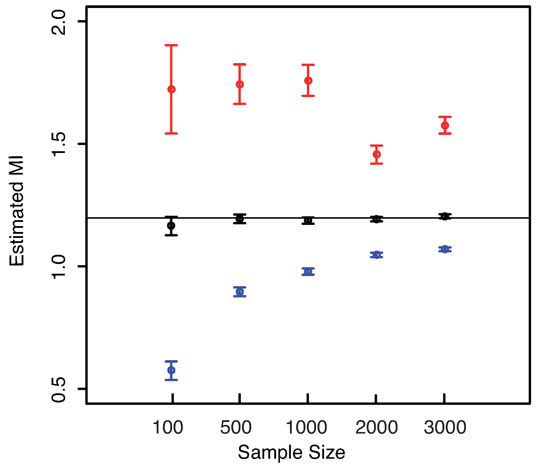
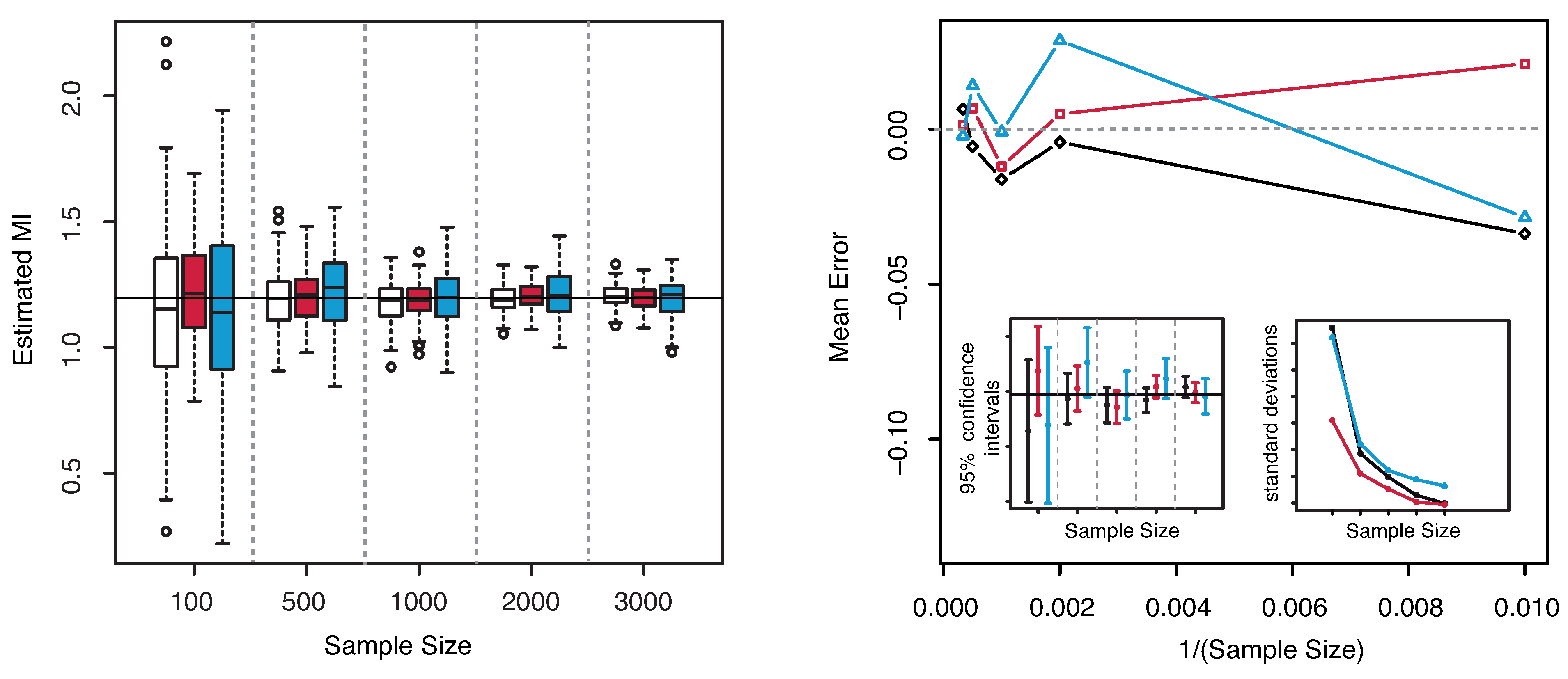
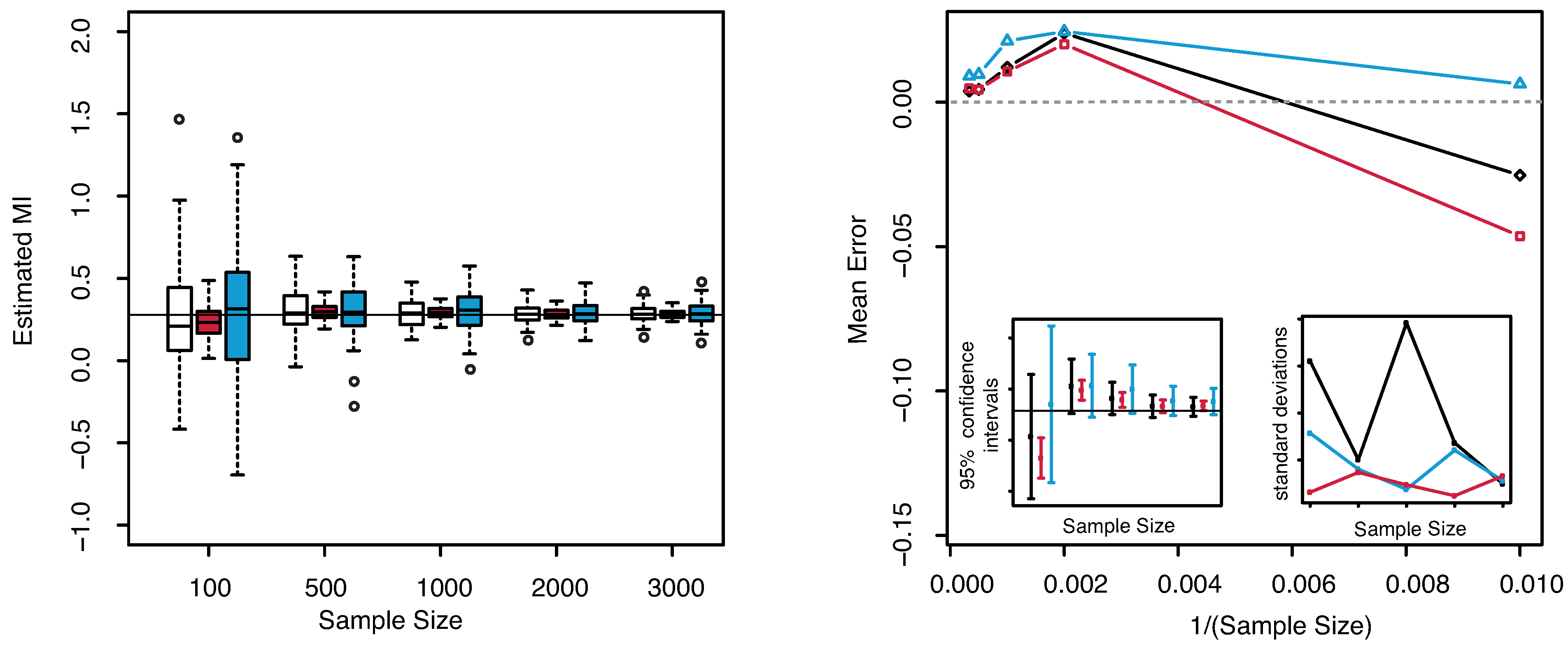
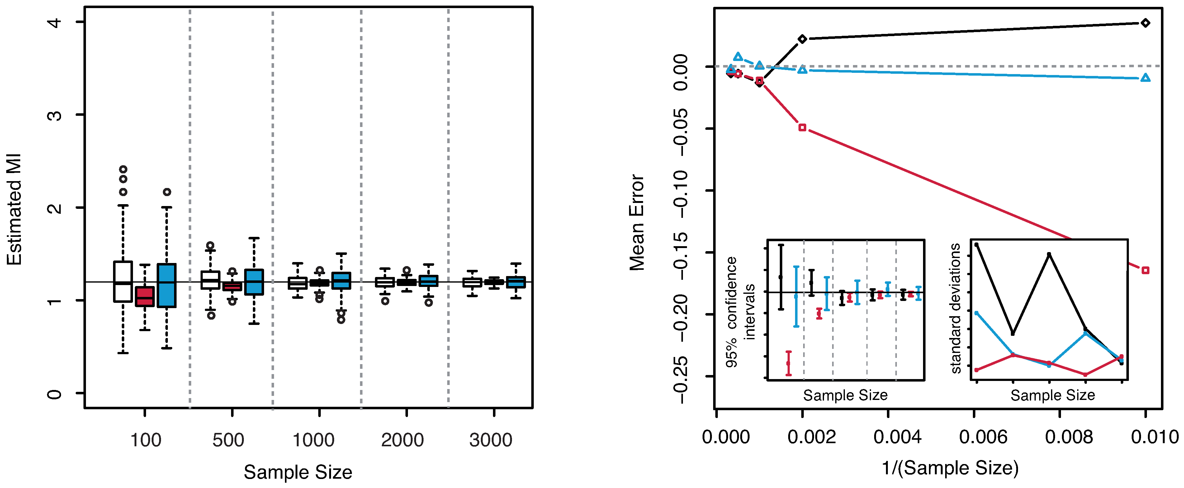
The numerical results are illustrated in Figure 3. The horizontal line indicates the exact value $MI=1.1980$. Both plots reveal that our estimator of the MI is centered around its true value. The interquartile range considerably decreases with increasing sample size, becoming minimal for $n=3000$. The comparison of the performances with the KSG and “plain entropy” estimators shows that our method performs comparably with KSG except for very small sample sizes ($n=100$), where it has a larger dispersion, see Figure 3—right panel—bottom right inset. It results even better for the highest sample sizes. However its variance quickly decreases to the values attained by the KSG estimator that are sensibly smaller that the variances of the “plain entropy” method. Actually, the “plain entropy” estimator leads to poorer performances such as larger interquartile range and less marked centering of the confidence interval around the true value.

Figure 3. (Example 1) Left panel: Boxplots of the estimated MI grouped according to different sample sizes. Right panel: mean error as a function of $1/$(Sample Size). Insets to the right panel: 95% confidence interval for the estimated MI (bottom left) and standard deviations (bottom right) versus Sample Size. Color map: black and white for the estimator we propose in Section 3.2, red for KSG and blue for “plain entropy”.

Figure 3. (Example 1) Left panel: Boxplots of the estimated MI grouped according to different sample sizes. Right panel: mean error as a function of $1/$(Sample Size). Insets to the right panel: 95% confidence interval for the estimated MI (bottom left) and standard deviations (bottom right) versus Sample Size. Color map: black and white for the estimator we propose in Section 3.2, red for KSG and blue for “plain entropy”.

• Example 2. Let $X_1$ and $X_2$ be linearly dependent random variables, related through the following equation

  $$X_2=5X_1+X_3$$

  where $X_1$ is uniformly distributed on the interval $[0,1]$ and $X_3$ is a standard gaussian random variable. In this case the mutual information is proved to be $MI=0.7961$ bit, see [33].

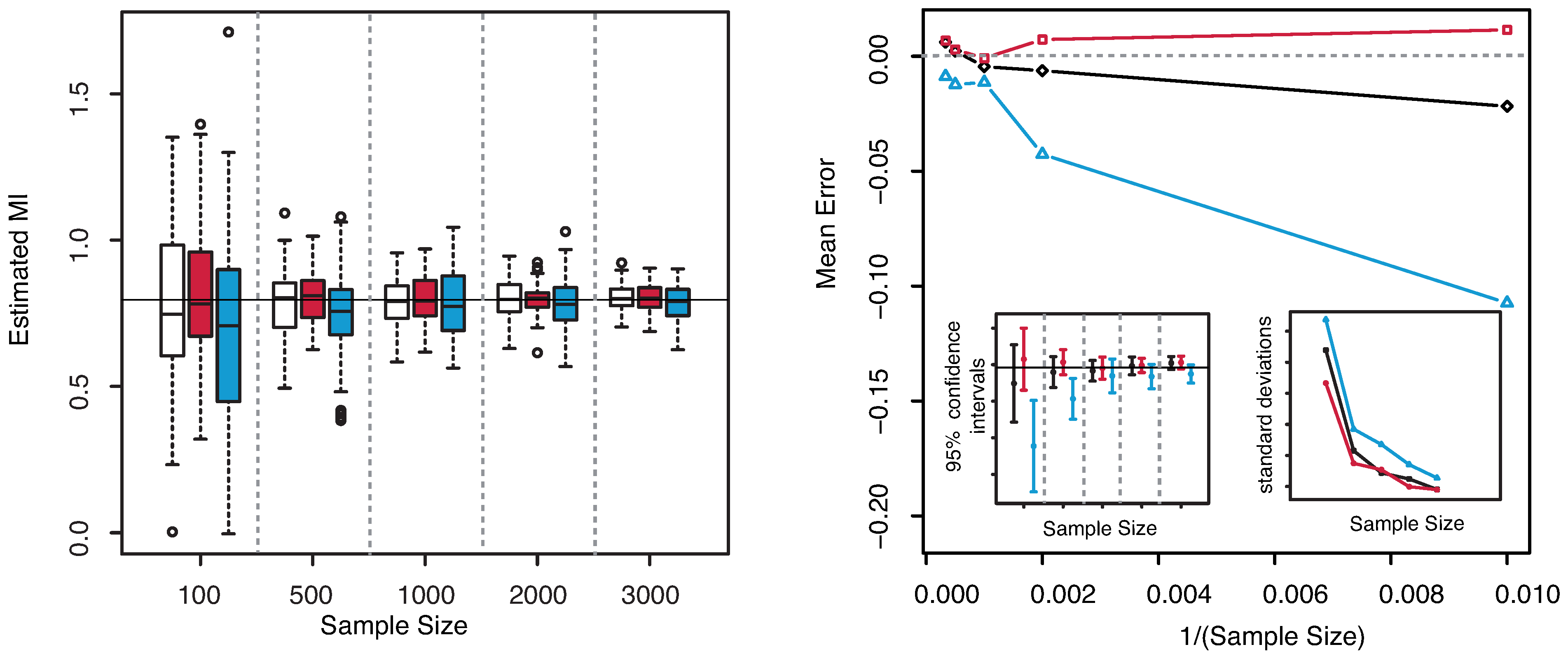
The numerical results are illustrated in Figure 4. Similar observations as for the previous example can be deduced for this case. The dispersion is clearly highly reduced as the sample size increases, but the estimated MI is always centered with respect to the true value. The “plain entropy” method is again less performing with respect to the others both in terms of dispersion and of centering the true value. The standard deviations of the estimates obtained with our method appear always lower than the ones obtained with the “plain entropy” method and comparable with those obtained by KSG method except for very small sample sizes $N=100$.

Figure 4. (Example 2) Left panel: Boxplots of the estimated MI grouped according to different sample sizes. Right panel: mean error as a function of $1/$(Sample Size). Insets to the right panel: 95% confidence interval for the estimated MI (bottom left) and standard deviations (bottom right) versus Sample Size. Color map: black and white for the estimator we propose in Section 3.2, red for KSG and blue for “plain entropy”.

Figure 4. (Example 2) Left panel: Boxplots of the estimated MI grouped according to different sample sizes. Right panel: mean error as a function of $1/$(Sample Size). Insets to the right panel: 95% confidence interval for the estimated MI (bottom left) and standard deviations (bottom right) versus Sample Size. Color map: black and white for the estimator we propose in Section 3.2, red for KSG and blue for “plain entropy”.

• Example 3. Let $X_1$,$X_2$ have joint c.d.f. given in the following equation

  $$F_{1,2}(x_1,x_2)=\left\{\begin{array}{c}\frac{(x_1+1)(e_2^x-1)}{x_1+2e_2^x-1}(x_1,x_2)\in [-1,1]\times [0,\infty ]\\ 1-e^{-x_2}(x_1,x_2)\in (1,\infty ]\times [0,\infty ]\end{array}\right.$$

  with components that are respectively a uniform random variable on the interval $[-1,1]$ and an exponential random variable with unitary parameter. In this case the copula function can be obtained in closed form (see [20])

  $$C(u_1,u_2)=\frac{u_1{u}_2}{u_1+u_2-u_1{u}_2}$$

  (40)

  which corresponds to the copula density function

  $$c(u_1,u_2)=\frac{2u_1{u}_2}{{(u_1+u_2-u_1{u}_2)}^3}$$

  A numerical integration then allows to obtain the mutual information $MI=0.2787$ bit.

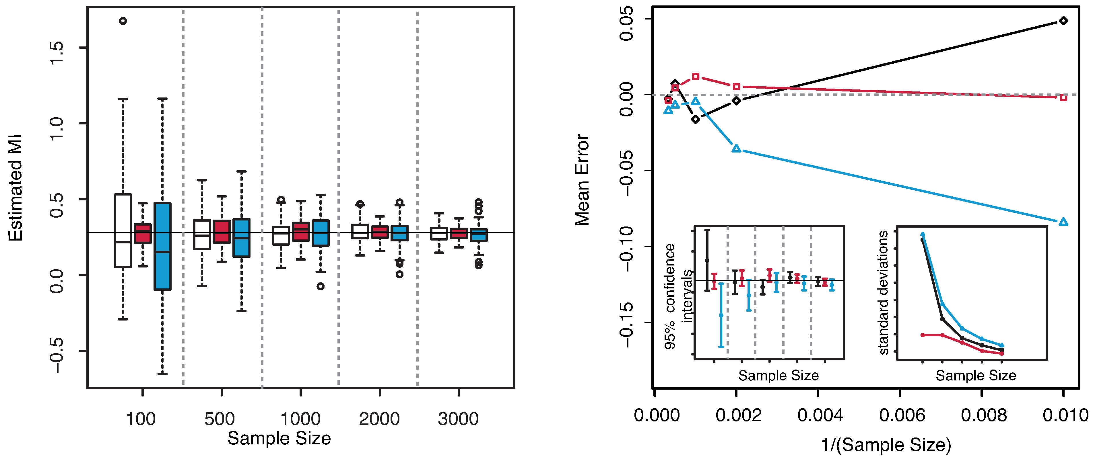
Both the boxplots and the confidence intervals in Figure 5 show that the values of MI obtained with our estimator are centered around the true value even for the smallest sample sizes $n=100$ and $n=500$. The comparison with KSG and “plain entropy” methods in Figure 5—right panel shows that the method proposed allows to obtain results that are comparable with the first one apart only for $n=100$ and is always better performing than the second one. This last method produces not centered estimates for small sample sizes such as $n=100$ and $n=500$. The standard deviations behave as in the previous example.

Figure 5. (Example 3) Left panel: Boxplots of the estimated MI grouped according to different sample sizes. Right panel: mean error as a function of $1/$(Sample Size). Insets to the right panel: 95% confidence interval for the estimated MI (bottom left) and standard deviations (bottom right) versus Sample Size. Color map: black and white for the estimator we propose in Section 3.2, red for KSG and blue for “plain entropy”.

Figure 5. (Example 3) Left panel: Boxplots of the estimated MI grouped according to different sample sizes. Right panel: mean error as a function of $1/$(Sample Size). Insets to the right panel: 95% confidence interval for the estimated MI (bottom left) and standard deviations (bottom right) versus Sample Size. Color map: black and white for the estimator we propose in Section 3.2, red for KSG and blue for “plain entropy”.

• Example 4. Let $(X_1,X_2)$ be a bivariate lognormal random vector with zero mean and covariance matrix given by

  $$Cov(X_1,X_2)=\frac{1-e^{-2\beta T}}{2\beta }\Sigma =\frac{1-e^{-2\beta T}}{2\beta }\left(\begin{array}{cc}1& 0.9\\ 0.9& 1\end{array}\right)$$

  with $\beta =0.1$ and $T=2$. Let us notice that the random vector $(X_1,X_2)$ can be interpreted as a two–dimensional geometric Ornstein–Uhlenbeck (OU) process at the time $T=2$, see [34]. The numerical value of the mutual information in this case is again $MI(X_1,X_2)=1.1980$ bit, as in the Example 1. Indeed the random vector $(X_1,X_2)$ can be obtained as the exponential of the bivariate OU process at time $T=2$, that is a Gaussian random vector. As MI is invariant under reparametrization of the marginal distributions and in the Gaussian case (with components with equal variances) depends only on the covariance structure, we get the same value as in the previous example.

The results are illustrated in Figure 6. The methods are applied to samples drawn from the joint distribution of $(X_1,X_2)$ with no pre–processing. Our approach gives good results both in terms of centered confidence intervals and standard deviations. Hence the method is robust to this kind of heavy–tailed distributions. The KSG estimator gives bad results for smaller sample sizes ($N=100,500,1000$) as the corresponding confidence intervals do not include the true value of MI. The “plain entropy” method seems to behave perfectly in this case.

Figure 6. (Example 4) Left panel: Boxplots of the estimated MI grouped according to different sample sizes. Right panel: mean error as a function of $1/$(Sample Size). Insets to the right panel: 95% confidence interval for the estimated MI (bottom left) and standard deviations (bottom right) versus Sample Size. Color map: black and white for the estimator we propose in Section 3.2, red for KSG and blue for “plain entropy”.

Figure 6. (Example 4) Left panel: Boxplots of the estimated MI grouped according to different sample sizes. Right panel: mean error as a function of $1/$(Sample Size). Insets to the right panel: 95% confidence interval for the estimated MI (bottom left) and standard deviations (bottom right) versus Sample Size. Color map: black and white for the estimator we propose in Section 3.2, red for KSG and blue for “plain entropy”.

• Example 5. Let $(X_1,X_2)$ be a random vector with Levy distributed margins, i.e., with p.d.f. given by

  $$f(x,\mu ,c)=\sqrt{\frac{c}{2\pi }}\frac{e^{-\frac{c}{2(x-\mu )}}}{{(x-\mu )}^{3/2}}$$

  with $\mu =0$ and $c=0.5$ and coupled by the same copula function introduced in Equation (40). Hence the mutual information is again $MI=0.2787$ bit.

All the three methods fail in estimating MI in this case. The results are totally unreliable. The errors are very large even for larger sample sizes. Concerning our method the problem relies in the estimation of the density of the margins when the tail has strongly power law behavior. In this very ill–served example, the tails are so heavy that it is frequent to have values very far from those corresponding to the largest part of the probability mass and the kernel estimate is poor as it would need too many points. The kernel method fails and so the estimation of MI.

However we propose here to exploit the property of MI of being invariant under reparametrization of the margins. This trick allows to get rid of the heavy tail problems at least in some cases. For example, when the random variables are positive valued, we could apply a sufficiently good transformation of the values in order to improve the estimates. Such a transformation should be strictly monotone and differentiable and able to lighten and shorten the tails of the distribution, as the logarithm function. In Figure 7 we illustrate the results obtained on samples drawn from the couple $(X_1,X_2)$ with Levy margins and pre–processed applying a log–transformation to the values. Such a procedure will not affect the estimated value, as it can be seen in the figure. All the three methods now give correctly estimated values.

Figure 7. (Example 5) Left panel: Boxplots of the estimated MI grouped according to different sample sizes. Right panel: mean error as a function of $1/$(Sample Size). Insets to the right panel: 95% confidence interval for the estimated MI (bottom left) and standard deviations (bottom right) versus Sample Size. Color map: black and white for the estimator we propose in Section 3.2, red for KSG and blue for “plain entropy”.

Figure 7. (Example 5) Left panel: Boxplots of the estimated MI grouped according to different sample sizes. Right panel: mean error as a function of $1/$(Sample Size). Insets to the right panel: 95% confidence interval for the estimated MI (bottom left) and standard deviations (bottom right) versus Sample Size. Color map: black and white for the estimator we propose in Section 3.2, red for KSG and blue for “plain entropy”.

Hence the method is shown to be only partly robust to heavy–tailed distributions, as KSG and “plain entropy”. In particular it succeeds when applied to distributions with tail behavior as in the log–normal case and fails on strong power law tailed distributions as the Levy one. However, in the latter case, our proposal is to take advantage of the invariance property of MI and to pre–process data in order to reduce the importance of the tails. This comment holds good for any dimension $d>2$, as the examples shown in the next section.

4.2. Three-Dimensional Vectors

We tested our estimator also in the case $d=3$, considering the multi–indices given in Equation (31). Let $X=(X_1,X_2,X_3)$ be a gaussian random vector with standard normal components and pair correlation coefficients ${\rho }_{X_1,X_2}={\rho }_{X_2,X_3}={\rho }_{X_1,X_3}=0.9$. The exact MI can be evaluated by means of the following equation

$$MI=\frac{1}{2}{log}_2\left(\frac{det\left({\sigma }_{(X_2,X_3)}\right)}{det\left({\sigma }_X\right)}\right)$$

where ${\sigma }_Y$ denotes the covariance matrix of the random vector Y. In the specific case we get $MI=1.3812$ bit.

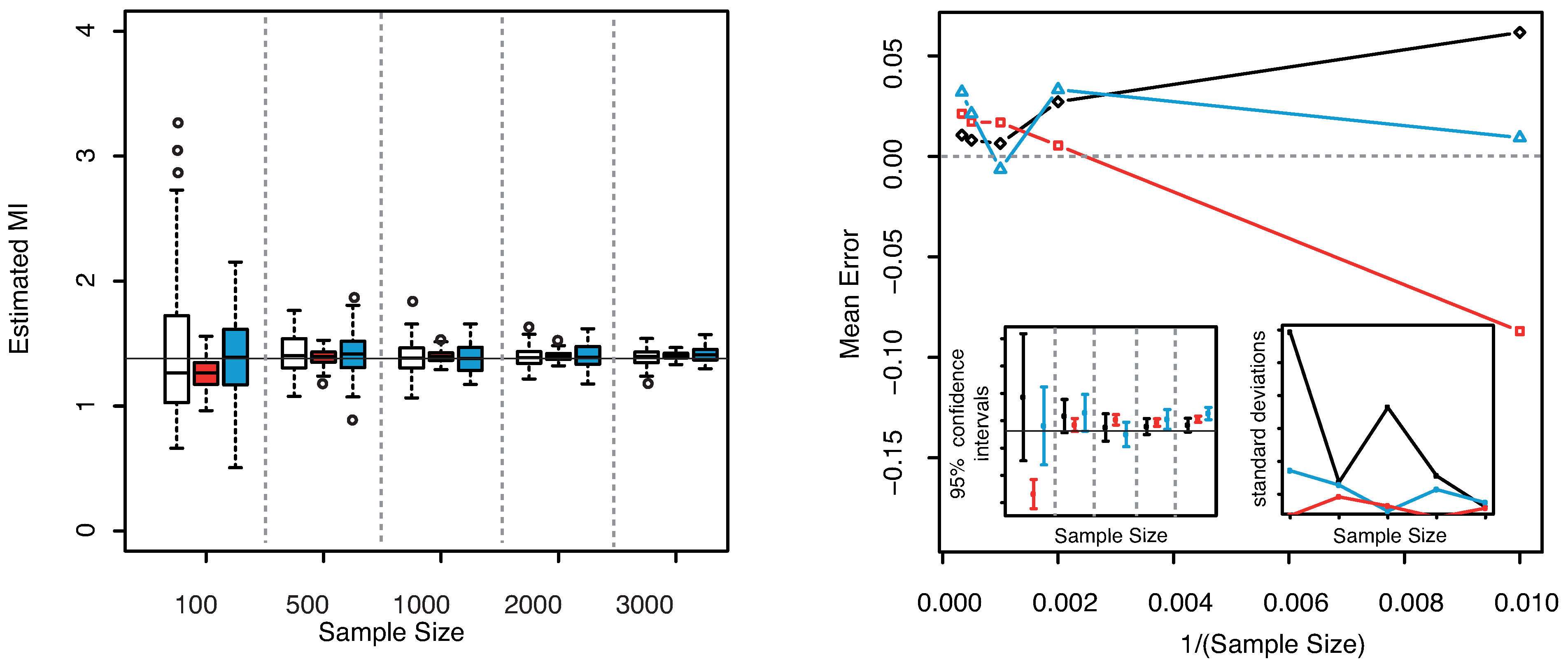
In Figure 8—left panel we show the boxplots of the estimated MI values as the sample size increases. From both plots the unbiasedness of the estimator even for small sample sizes can be clearly detected. Our estimator always leads to better results than the others both for unbiasedness and for the dispersion, cf. Figure 8—right panel. Both the KSG and the “plain entropy” estimator do not center the exact value of the MI for the largest sample sizes ($n=2000$ and $n=3000$), even though the standard deviations are comparable with the ones obtained with our method.

Figure 8. (Gaussian $d=3$) Left panel: Boxplots of the estimated MI grouped according to different sample sizes. Right panel: mean error as a function of $1/$(Sample Size). Insets to the right panel: 95% confidence interval for the estimated MI (bottom left) and standard deviations (bottom right) versus Sample Size. Color map: black and white for the estimator we propose in Section 3.2, red for KSG and blue for “plain entropy”.

Figure 8. (Gaussian $d=3$) Left panel: Boxplots of the estimated MI grouped according to different sample sizes. Right panel: mean error as a function of $1/$(Sample Size). Insets to the right panel: 95% confidence interval for the estimated MI (bottom left) and standard deviations (bottom right) versus Sample Size. Color map: black and white for the estimator we propose in Section 3.2, red for KSG and blue for “plain entropy”.

4.3. Four-Dimensional Vectors

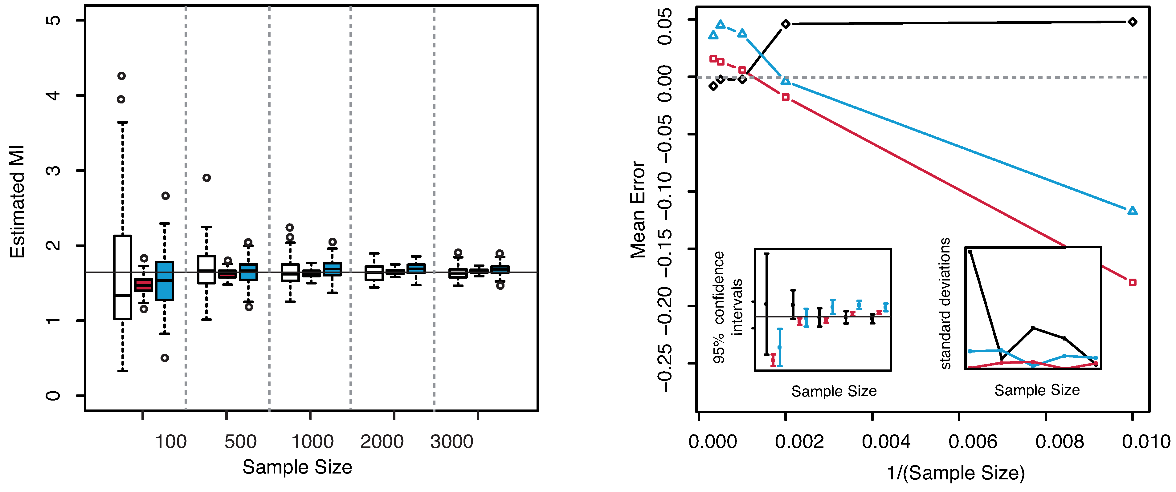
For the case $d=4$ we considered a multivariate Gaussian random vector with mean and covariance matrix given as

$$\begin{array}{c}\hfill \mu =(0,0,0,0)\Sigma =\left(\begin{array}{cccc}1& 0.9& 0.9& 0.9\\ 0.9& 1& 0.9& 0.9\\ 0.9& 0.9& 1& 0.9\\ 0.9& 0.9& 0.9& 1\end{array}\right)\end{array}$$

We chose the following multi–indices to group the components: ${\alpha }^1=(1,2)$ and ${\alpha }^2=(3,4)$. The results are illustrated in Figure 9. As already noticed for the three dimensional Gaussian case, the KSG and “plain entropy” estimators seems biased while the estimator here presented centers the true value for all the explored sample sizes.

Figure 9. (Gaussian $d=4$) Left panel: Boxplots of the estimated MI grouped according to different sample sizes. Right panel: mean error as a function of $1/$(Sample Size). Insets to the right panel: 95% confidence interval for the estimated MI (bottom left) and standard deviations (bottom right) versus Sample Size. Color map: black and white for the estimator we propose in Section 3.2, red for KSG and blue for “plain entropy”.

Figure 9. (Gaussian $d=4$) Left panel: Boxplots of the estimated MI grouped according to different sample sizes. Right panel: mean error as a function of $1/$(Sample Size). Insets to the right panel: 95% confidence interval for the estimated MI (bottom left) and standard deviations (bottom right) versus Sample Size. Color map: black and white for the estimator we propose in Section 3.2, red for KSG and blue for “plain entropy”.

5. Conclusions

In this paper, we have presented a new estimator for the mutual information between subsets of components of d-dimensional random vectors. It exploits the link between the mutual information and the entropy of the linkage function here proved. Hence the problem of estimating mutual information is reduced to the computation of the entropy of a suitably transformed sample of uniformly distributed random variables on the interval $[0,1]$, that can be easily performed by the k–nearest neighbor technique illustrated in [10].

The method gives very good performances in terms both of unbiasedness and variance of the estimates. For the 2–dimensional case, the results are comparable to the KSG and “plain entropy” estimates. However, for higher dimensions (we tested on examples up to dimension 4), our method is preferable as it keeps being centered while KSG and “plain entropy” both show a bias. All the tested estimators are shown to be robust for mild heavy tailed distributions, such as the lognormal distribution, but they fail on distributions with power law tail probabilities and no finite moments, such as the Levy distribution. However, we suggest to overcome the problem using the invariance property of MI under reparametrization of the margins and hence pre–processing the data with a suitable transformation of the univariate components before estimation.

The fact that the estimator gives unbiased results for small sample sizes and larger dimensions allows a wide use, also in applications where the availability of big data sets from real experiments is extremely rare.