Article

Core-Based Dynamic Community Detection in Mobile Social Networks

Science and Technology on Information Systems Engineering Laboratory, National University of Defense Technology, Changsha 410073, Hunan, China
*
Author to whom correspondence should be addressed.
Entropy 2013, 15(12), 5419-5438; https://doi.org/10.3390/e15125419
Submission received: 12 September 2013 / Revised: 21 November 2013 / Accepted: 21 November 2013 / Published: 6 December 2013
(This article belongs to the Special Issue Social Networks and Information Diffusion)

Abstract

:
The topic of community detection in social networks has attracted a lot of attention in recent years. Existing methods always depict the relationship of two nodes using the snapshot of the network, but these snapshots cannot reveal the real relationships, especially when the connection history among nodes is considered. The problem of detecting the stable community in mobile social networks has been studied in this paper. Community cores are considered as stable subsets of the network in previous work. Based on these observations, this paper divides all nodes into a few of communities due to the community cores. Meanwhile, communities can be tracked through incremental computing. Experimental results based on real-world social networks demonstrate that our proposed method performs better than the well-known static community detection algorithm in mobile social networks.

Graphical Abstract

1. Introduction

In recent years, the way people communicate has experienced dramatic changes. Thanks to the development of mobile communication technology, the relative geographical topology of people can be easily determined. Hence, clustering people in such mobile social network, which can be further used in information recommendation and other social services, has attracted more and more research interest.
There is a lot of literature concerning the topic of community detection in social networks, including static and dynamic approaches. Nodes are usually depicted as people in the real world, and links are denoted to the contacts among nodes. The static approaches focus on high aggregation of nodes which have same features [1,2], while the dynamic approaches divide the network's evolving process into a few of timestamps, not only paying attention to the degree of aggregation, but also to the computational complexity at each timestamp [3,4]. However, few of these methods consider the stability of communities between two timestamps. Intuitively, in our real world, the relationship among people will not change sharply. Seifi [5] considered the stability in community detection, but tried to obtain a community partition in a stable modularity scenario, rather than stable contact.
Moreover, Pan [6] has pointed out that inter-contact time among people follows the power-law distribution, which means: (1) we spend most of our time contacting with the “community” people; (2) there are a few temporary contacts between “strangers”. If all of links are considered when detecting a community, some “temporary links” among “strangers” will influence the effect. In order to eliminate the negative influence, only “familiar links” should be concerned. Then, the key problem is: how to find the stable communities through “familiar links” in mobile social networks?
The biggest feature of mobile social networks is that nodes and links are always changing. Researchers [3,7] have classified all of the situations that occur at each timestamp into several events, including node addition/removal and link addition/removal. Their experiment results demonstrate that discretization of the continuous time is a useful way to model the evolution of a network. In this paper, the discretization of the continuous time is still adopted when modeling the evolution process, but the prominent difference of our method compared with others is the discrimination between “familiar link” and “temporary link”.
Based on previous works [8], the number of “familiar links” is higher than that of “temporary links”. In other words, people who come from the same community have higher contact frequency than those who come from different communities. The frequency of change of “familiar links” is lower than that of “temporary links”, that is to say, the people coming from the same community always maintain relatively stable contacts, while contacts among people who come from different communities seem to be uncertain.
This paper uses the concept of “community core” to solve the problem above, which is based on the previous work described in [9]. Community cores are subsets of nodes in the network. On the one hand, nodes in community cores have more stable links than outside. On the other hand, the number of community cores is stable. Based on community cores, all nodes in the network can be divided into a few communities, then the community partition can be obtained.
Due to the dynamic features of many social networks [10], community evolution has attracted much research attention in recent years. Current research on community evolution involves the following categories: evolutionary clustering [11,12,13] usually aims to find an optimal cluster sequence by finding a clustering at each timestamp that optimizes the incremental quality. Meanwhile, probabilistic models and parameter estimation methods have also been proposed [14,15]. Non-negative matrix factorization was introduced to evolution analysis [16] as well. Besides these algorithms concerned with the evolution procedures of communities, community detection in dynamic social networks aims to detect the optimal community partition at each timestamp [4,7,17,18,19]. Moreover, in order to describe the change of communities at different timestamps, tracking algorithms [20,21] based on similarity comparison have also been studied.
In this paper, we study the characteristics of human contacts first, especially the cumulative contact. Then, a novel approach for community detection in mobile social networks is proposed. Moreover, in order to recognize the changes of communities at each timestamp, the tracking mechanism is also discussed. To the best of our knowledge, we are the first to find the relatively stable community using the cumulative contact history in mobile social networks, and the first to find the power-law distribution of these contacts” changing between consecutive timestamps.
The rest of this paper is organized as follows: we introduce the preliminaries used in this paper in Section 2. In Section 3, we discuss the character of cumulative stable contact. Then, we present our community core detection and tracking algorithm separately in Section 4. We evaluate our algorithms in Section 5, and finally conclude the work in Section 6.

2. Preliminary

In this section, we present the notion and the mobile network model that we will use throughout the paper.
Definition 1 (Mobile Social Network) A mobile social network is denoted as G = (E,V), where V is the vertex set and E the link set. Topologies of mobile social networks are always changing due to the time variation, which is the main difference compared with static networks. Like previous works, we treat the continuous time as a sequence of timestamps. Furthermore, nodes and links may be different in the consecutive timestamps. Hence, we use the following four events to describe the evolution of network: node add, node remove, link add, link remove.
Definition 2 (Cumulative Stable Contact, CSC) The cumulative stable contact is denoted as the historic contact duration which is higher than a threshold (we will discuss this threshold in the following section). As mentioned before, the temporary link cannot depict the relationship between two nodes in the mobile social network. Inversely, two nodes disconnect at T = t cannot demonstrate that they are irrelevant. Considering the history connection among nodes, we use cumulative contact to judge the stability of links.
Definition 3 (Community) A group of nodes in the network which have higher contact frequency. Different from existing definition of community, we aim to find the stable communities in the network, so the contact frequency is considered when detecting communities.
Definition 4 (Community Core) The community cores are the subset of communities. Nodes in community cores have higher contact frequency, and few changes will occur as time changes.

3. Cumulative Stable Link

In this section, we study the character of CSC. First, a well-known mobile social network is introduced. Then a stable link extraction method is proposed to find the CSC. Finally, we discuss the distribution about the Change of CSC (CCSC).

3.1. Dataset

Due to the increasing interest in mobile social networks, various datasets about people’s behavior have been collected. Researchers have separately collected, for example, the traces information about attendees at INFOCOM06 [8] and SIGCOMM09 [22]. The features of these datasets are as follows: (1) these datasets include not only the contact information but also the attributes of attendees. SIGCOMM09 had 76 attendees and INFOCOM06 had 78 attendees; (2) both of these datasets contain several days of traces information, and more than 300,000 timestamps can be used to describe the evolution of the networks.
SIGCOMM09 collects the traces information among attendees at SIGCOMM 2009. The dataset not only records the contact time of each device pair, but also includes the profile of each attendee such as country, city, institution, interests etc. The most important information is the friendship mentioned by attendees at the beginning of the experiment, which is used as the basic friendship graph in this paper. The contact information is recorded in the form of <timestamp; user_id; seen_user_id; device_major_cod; device_minor_cod>, and the cumulative contact pair at each timestamp is easier to obtain.
Like SIGCOMM09, INFOCOM06 collects the contact traces among attendees at INFOCOM 2006. Each participant was asked to fill a questionnaire including name, nationality, affiliation, country, etc. The contact information is also well refined by the author so that it is in the form of <user_id, seen_user_id, start time, end time, ...>. Only the front four columns are used in this paper.

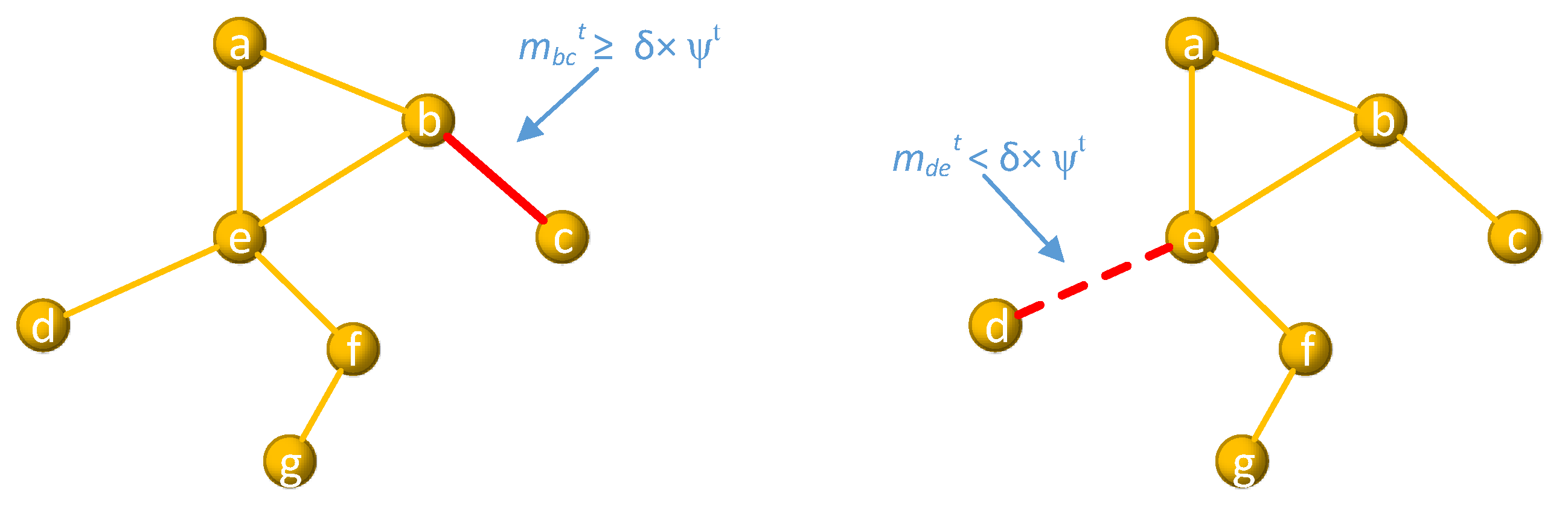
3.2. Stable Link Extraction

Both the SIGCOMM09 and INFOCOM06 datasets contain connection duration between each pair of nodes. We use a contact matrix M denoting the contact among nodes. m i , j t is the cumulative contact duration between vi and vj from T = 0 to T = t. We use ψt denoting the maximum elements of M at T = t.
Pan [8] has studied the correlation between regularity and familiarity on Cambridge students, and it was observed that most of contacts among nodes reveal a short duration, while few of them have long duration, which is denoted as “community”. In this paper, we use M' = [m'i,j] to denote whether vi and vj have a contact duration higher than a threshold δ·ψt. Then we cluster the attendees into several groups by their friendship graphs which are extracted from the two datasets:
m i j = { m i j t   ,   m i j t δ · ψ t   0   ,   m i j t < δ · ψ t

3.3. Distribution of CCSC

We first construct a contact duration matrix M = [mi,j], where mi,j presents the history of the contact duration between vi and vj during the whole lifetime of the network (INFOCOM06: T [6207, 340927], SIGCOMM09: T [21, 349811]). Without loss of generality, we denote X and Y as two consecutive M, then compute the Change of History Contact (CHC), which is depicted as the distance of X and Y using:
D i s t a n c e ( X , Y ) = j i s ( i , j ) ,   s ( i , j ) = { 0   ,   X i j = Y i j 1   ,   X i j Y i j
In order to avoid the mismatching caused by different sizes of X and Y, all of nodes in the networks are included in contact duration matrix. The distribution of the distance is plotted on a log-log scale (Figure 1). The power-law distribution of inter-contact time in the mobile social network is fully discussed in existing literatures, however, the change of contacts at consecutive timestamps does not follow the power-law distribution. Then, we use M', where m'i,j denotes wether a link between vi and vj is a CSC or not, and compute the distance of two consecutive M', then the CCSC at different timestamps is obtained (Figure 1). It is clear that the CCSC extracted from SIGCOMM09 follows the power-law distribution, and ranges from two changes to six changes. In INFOCOM06, when the changes range from two to seven, the CCSC also follows the power-law distribution. The diversity of distribution between historic contact duration and cumulative stable contact changes might be caused by removal of the temporary contact. Considering two people in the real world, the more familiar, the more stable their relationship is. Moreover, people denoted as “familiar” have longer contact duration and contact time, which has been proven in previous works. According to the discussion above, the CSC removes the temporary links among nodes, which can be used in the community detection.
Figure 1. (a) Distribution of Contact Duration History; (b) Distribution of CCSC.
Entropy 15 05419 g001

4. Core-based Community Evolution

In this section, a core-based community evolution mechanism named CoCE is presented. We first introduce the community detection algorithm, then discuss the community tracking mechanism in mobile social networks.

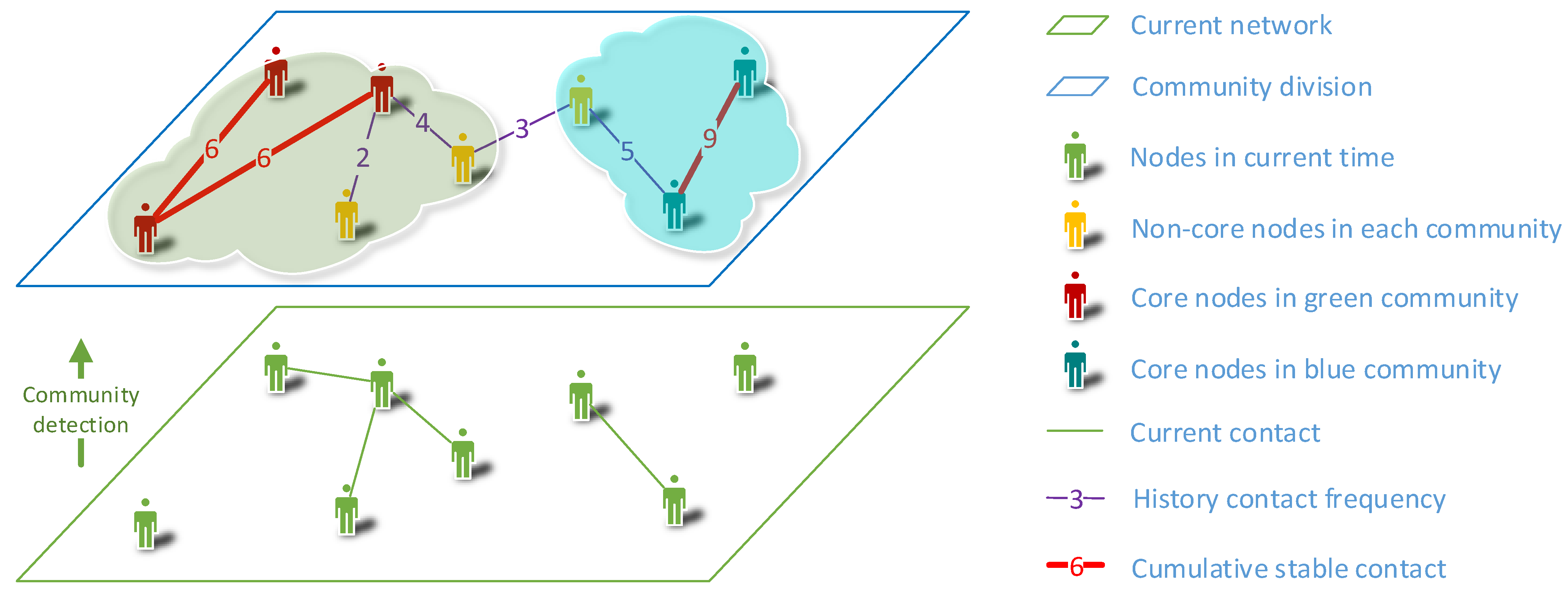
4.1. Core based Community Detection

In order to find the stable communities in the networks, the community detection algorithm will start when it detects the community core using the cumulative stable link. The community cores can be seen as the most stable subsets of communities. After that, the remaining nodes outside the community cores will join into community cores by the shortest distance [23]. Then the initial community division can be obtained. An example of this procedure is depicted in Figure 2.
Let’s first discuss the network topology change, which is constantly updated as nodes and links change through different timestamps. The increasing nodes or links can be decomposed as a sequence of node or link insertions, while the decreasing nodes or links can be decomposed as a sequence of node or link removals. We define four events that may cause the network evolution: node add, node remove, link add, link remove. However, the community core is based on links between two nodes. Hence, a single node which links to no CSC cannot exist in the community core. Then, we refine the events as follows (Figure 3).
Figure 2. Community detection procedure. Firstly, the cumulative stable contacts are extracted from the contact information history. Then the community cores are constructed from the cumulative stable contacts. Finally, nodes in the network join into cores, respectively. Because the cumulative contacts reveal the relationship among nodes during the long-term, while the current contacts reveal the relationship at the current timestamp. The community structure is different from the current network topology.
Entropy 15 05419 g002
Figure 3. Two events cause the structure variation of network. Left: a link between node b and c is added into the network because m b c t δ · ψ t . Right: a link between node d and e is removed from the network because m d e t < δ · ψ t .
Entropy 15 05419 g003
Link Add: the cumulative contact between vi and vj is higher than current threshold, then link ei,j associated with two nodes vi and vj adds to a community core. Both vi and vj will be added to the community core, even if none of them belong to community cores.
Link Remove: the cumulative contact between vi and vj is lower than the current threshold, then the link ei,j associated with two nodes vi and vj is removed from a community core. If vi or vj has no link associated with other nodes in the community core, then the corresponding node will be removed from the community core.
In order to detect communities at different timestamps, the CoCE adopts the incremental computation paradigm. At each timestamp, the variation of cumulative stable links will firstly be divided into two parts: the added link set and removed link set. Then, nodes in these two sets will be clustered into community cores, respectively. Finally, the remaining nodes in remaining node set will join into communities according to the shortest distance to each community core. The construction of communities is depicted in Figure 4, Figure 5 and Figure 6.
Figure 4. Link removing procedure.

Algorithm 1: Link Removal
While link removal set ≠ Ø
 Extract linkij from link removal set.
If vi and vj in the same core Then
  If vi and vj have a stable cumulative contact Then
   Remove linkij from existing community cores.
   If vi and vj connect with any other nodes Then
    If there is a path connects vi and vj Then
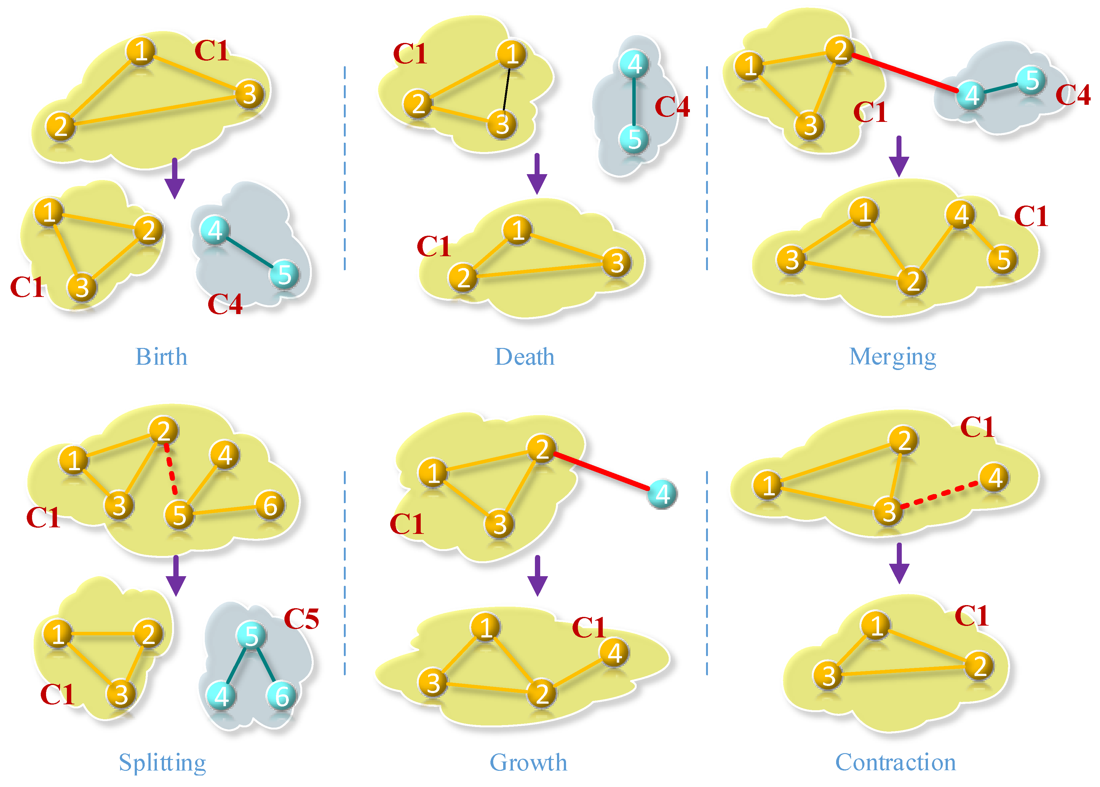
     Split the core into two parts, including vi and vj separately. (Splitting)
   Else If vi and vj don’t connect with any other nodes Then
    Remove vi and vj from cores. (Contraction or Death)
   Else If vi or vj doesn’t connect with any nodes Then
    Remove vi or vj which doesn’t connect with any nodes. (Contraction)
Figure 5. Link addition procedure.

Algorithm 2: Link Addition
While link addition set ≠ Ø
 Extract linkij from link addition set.
If vi and vj have a stable cumulative contact Then
  If vi and vj not in the same core Then
   If vi and vj have only one neighbor Then
    Create a new community core. (Birth)
   Else If vi or vj have one neighbor Then
    Merge the two cores. (Merging)
  Else
   Add linkij from existing community cores. (Growth)
Figure 6. Remaining nodes addition procedure.

Algorithm 3: Remaining Node Addition
While remaining node set ≠ Ø
 Extract vi from remaining node set.
If there is only one path from vi to any cores Then
  vi join into the connected core.
Else If there are multiple paths from vi to any cores Then
  vi join into the core which has the shortest distance to it.
Else
  A community is created including vi and nodes connected with vi.
The connectivity among nodes will be judged in the link removing algorithm, which operates in O(p+q) time, where p denotes the number of current vertexes and q denotes the number of current links. Supposing the worst situation in networks, the time complexity of the link removal algorithm at each time is O(u(p+q)), where u is the length of the link removal set. The complexity of the link addition algorithm is O(w), where w is the length of the link addition set. Finally, the remaining nodes addition algorithm needs to detect the shortest distance among nodes. Despite the optimal methods, the time complexity of the shortest distance detection algorithm is O(r3), where r is the number of nodes in the network. Hence, the total time complexity of our algorithms in the worst case are O(max{u(p+q), w, r3}) ~ O(r3). However, the complexity can be reduced through the optimal methods in shortest distance detection algorithms, which can be seen as a further improvement and will not be discussed in this paper.

4.2. Community Evolution

In order to study the ecommunity evolution process, we should track the communities at each timestamp. How to distinguish two communities in the consecutive timestamps is the biggest problem in this tracking.

4.2.1. Model

In previous literatures a broad consensus on the basic events that can be used to describe the evolution of dynamic communities can be seen [3,7,24]. We extend and specify these events-based cumulative stable contacts as follows (Figure 7):
Figure 7. Six community variation events. The red solid/dash line denotes the link addition and link removal separately, and different colors mean different communities. The community IDs are denoted as C1, C4, C5.
Entropy 15 05419 g007
Birth: There is a cumulative stable contact between two nodes, and the nodes belong to no communities before.
Death: A community is removed from an existing partition, which results from removal of the last cumulative stable contact in this community.
Merging: Two communities merge into one community because of the appearance of cumulative stable contact between nodes in different communities.
Splitting: A community is divided into two separate communities. Two sets of nodes connected by only one cumulative stable contact. Once the cumulative stable contact is removed from the network, nodes in the community will split into two communities.
Growth: A node joins a community, due to the appearance of cumulative stable contact between this node and nodes in communities.
Contraction: A node moves out of a community core, which is caused by the removal of cumulative stable contacts.

4.2.2. Tracking Communities

Community tracking can reveal the evolution procedure of communities. Existing methods usually use similarity measurement to identify communities between continuous timestamps. In order to express the evolution procedure more clearly, the label mechanism is proposed. Different from existing methods which track communities after the community detection using similarity measurement [21,24,25,26,27,28], our tracking algorithm tracks communities during the detection procedure. The goals of tracking algorithms are (Figure 8):
Figure 8. Goals of community tracking. NID denotes the node ID, and CID denotes the community ID. On the one hand, nodes in communities such as node N1 and N7 at each timestamp should be recognized, as well as their community IDs. On the other hand, community partition of the network at each timestamp should be acquired.
Entropy 15 05419 g008
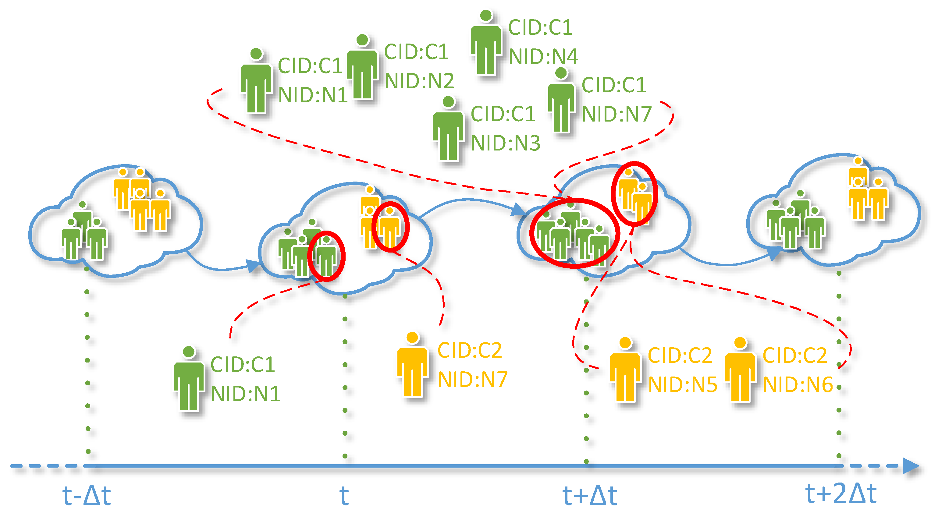
  • Any nodes’ community ID at any timestamps can be retrieved.
  • Members in any communities at any timestamps can be obtained.
Differing from existing methods, we track communities by enhancing our community detection algorithm. When the community detection algorithm runs, the tracking process works simultaneously, which is trigged by the variation of links.
According to the algorithm, only contact frequency between two core nodes lower than δ · ψ t are considered, and there is no other path connecting these two nodes in the original core, the splitting process will be triggered. Hence, vi and vj have their isolated communities separately. We use node ID as the community label when creating a new community. Initially, each node will be labeled a community ID by its node ID. The benefits are as follows: firstly, the finite namespace of community label will not cause naming confusion; secondly, communities can be tracked easier when they are created again. The tracking algorithm uses node ID as initial community ID.
Basic principles of tracking are as follows (which is depicted in Figure 7 as well):
Birth: The new community ID equals one of the member’s node ID.
Death: Members in community change their community ID to their node ID.
Merging: The community with less member changes its ID to the other community ID.
Splitting: Two communities change the IDs to one of their member’s node ID separately.
Growth: Increasing nodes change their community ID to an existing community ID.
Contraction: Reduced nodes change their community ID as their node ID.

5. Evaluation

In this section, we firstly discuss the stability of community cores which are detected by our algorithms (5.1–5.4). Then a comparison between our algorithms and a well-known algorithm named “COPRA” [27] is conducted (5.5–5.6).

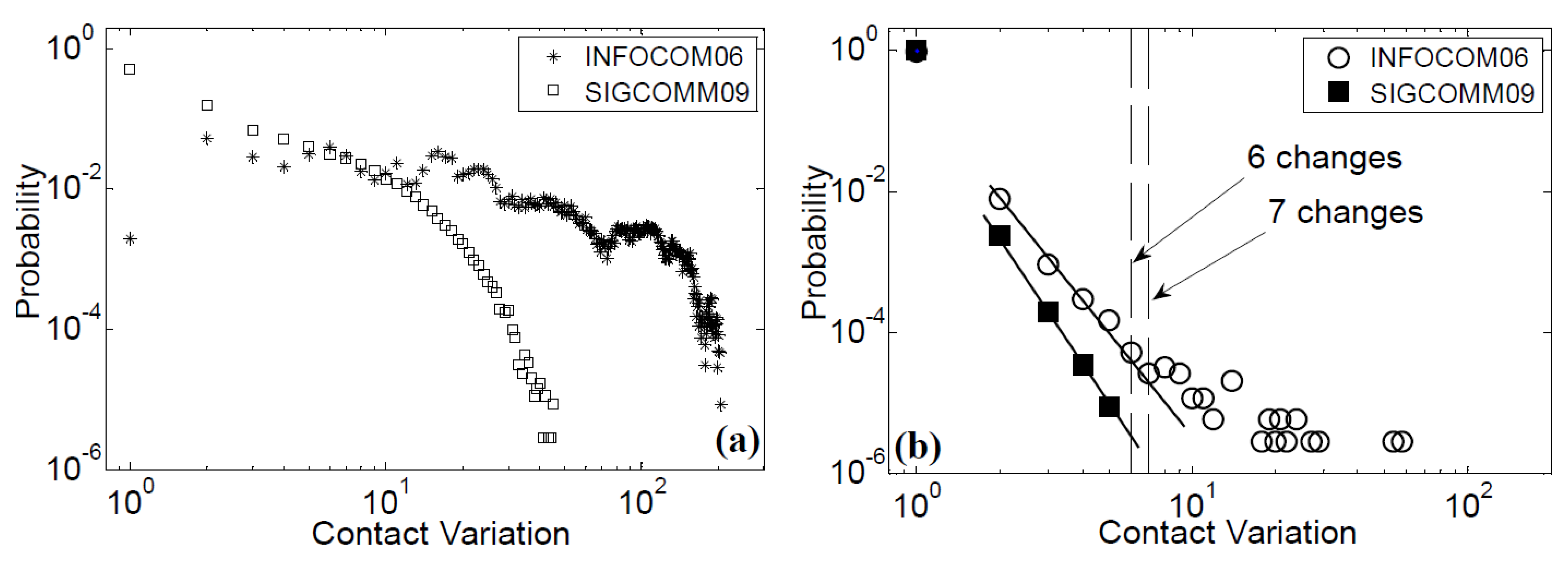
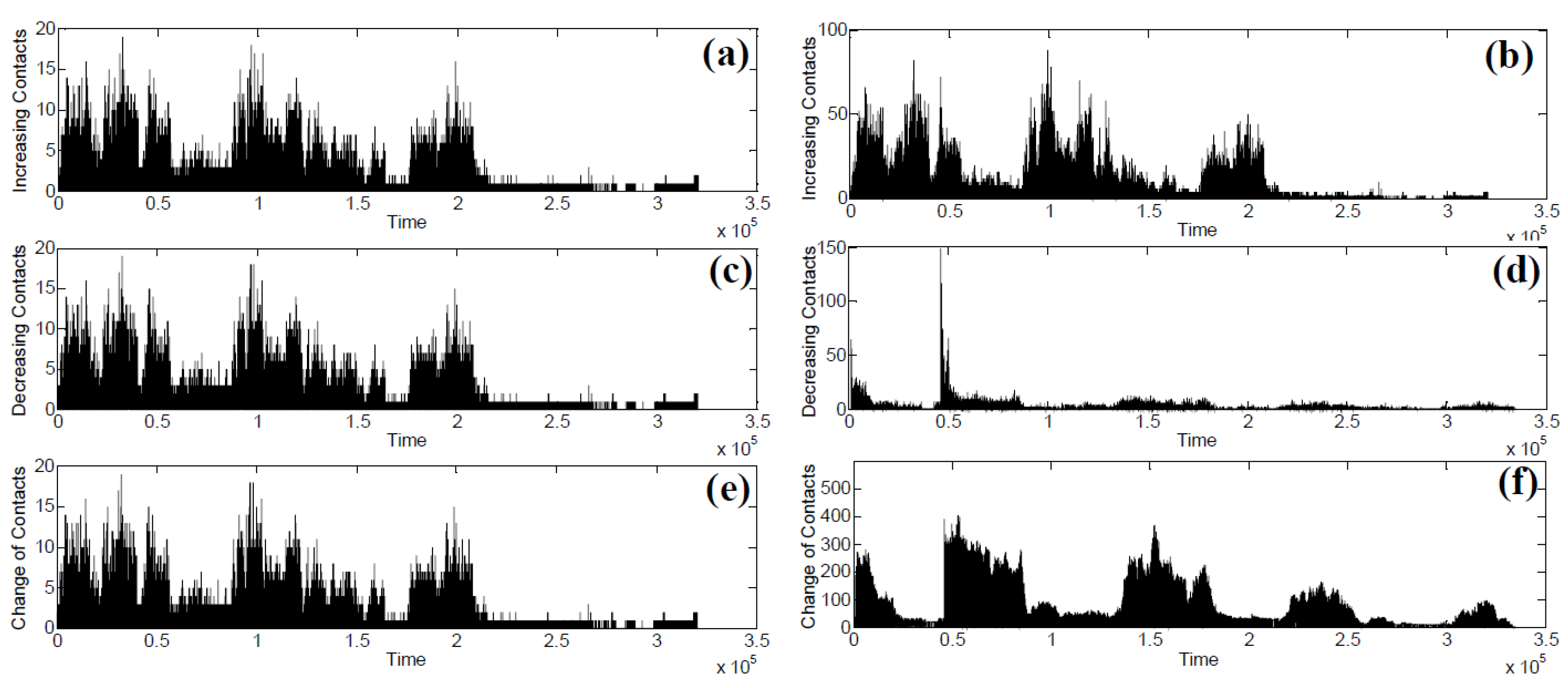
5.1. Contact Variation

In order to reveal the community core evolution briefly, we first show the contact variation of both SIGCOMM09 and INFOCOM06 over the whole lifetime (Figure 9). It is clear that the contact variation has a periodic feature. On the one hand, attendees have higher frequency of communication with each other during the daytime, this results in highly increasing and decreasing contacts. On the other hand, in the evening, the contact will not change as frequent as during the daytime. An interesting observation is that after about 60 hours (the third night), both of datasets have a low level of increasing and decreasing contacts, which means the positions of participants are relatively fixed.

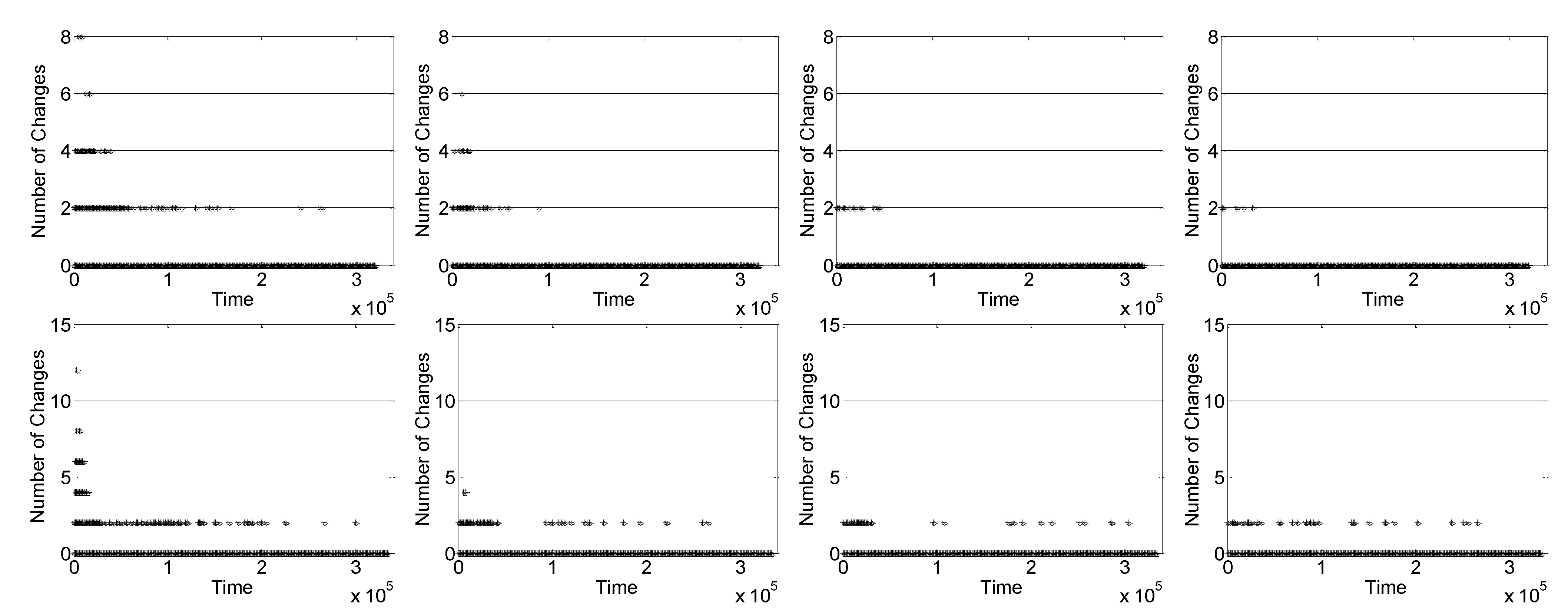
5.2. Change of 0–1 Contact Matrix

According to M', the 0-1 contact matrix B = [bi,j] can be obtained. M' changes as the time increases, and the maximum contact duration among nodes may be changed, which results to the variation of B: The change of B during the whole collection procedure is plotted in Figure 10:
b i j = { 1   ,   m i j t δ · ψ t   0   ,   m i j t = δ · ψ t
Figure 9. Description about two datasets. Left: link variation of SIGCOMM09, including (a) link add, (c) link remove and (e) total link change. Right: link variation of INFOCOM06, including (b) link add, (d) link remove and (f) total link change.
Entropy 15 05419 g009
Figure 10. Number of changes in 0-1 matrix between two consecutive timestamps. Above: number of changes in SIGCOMM09 under δ = 0.2, 0.4, 0.6, 0.8 (from left to right). Below: number of changes in INFOCOM06 under δ = 0.2, 0.4, 0.6, 0.8 (from left to right).
Entropy 15 05419 g010
The change of B during the whole collection procedure is plotted in Figure 10, where most of the changes occur at the beginning of collection, then gradually diminish over time. The number of changes reduces with increasing δ. Meanwhile, in SIGCOMM09, the maximum changes of the 0-1 contact matrix under δ = 0.2, 0.4, 0.6, 0.8 are 8, 6, 4 and 2 respectively, while in INFOCOM06, the values are 12, 4, 2 and 2. As δ increases, the maximum changes of the 0–1 contact matrix are reduced. The higher δ is, the more stable the contact matrix will be.

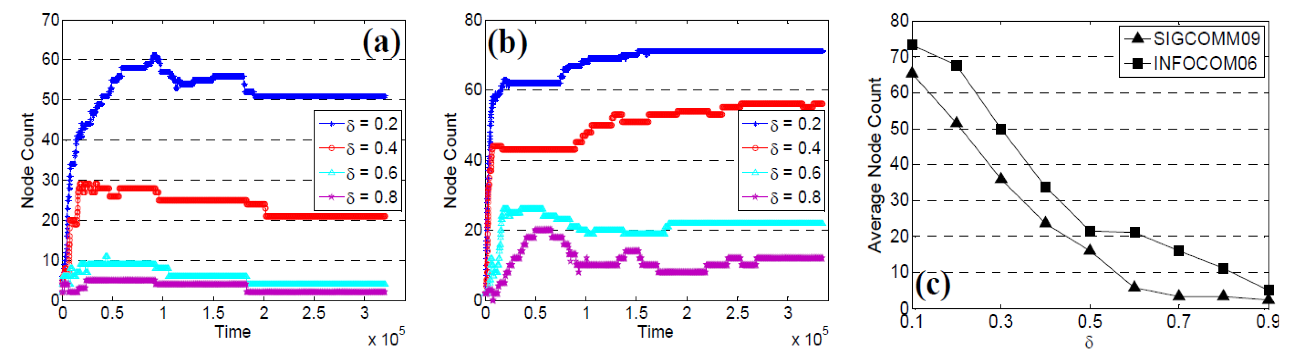
5.3. Selected Node Count

One of the biggest differences between communities and community cores is the number of clustered nodes. In other words, the community core of a mobile social network is a subset of the whole community. According to previous works [8], some nodes can be classified as “familiar strangers” and “friends”, and then the number of nodes in the “community” is even less. Hence, only the node pairs which have high contact frequency can be selected to the community core. Moreover, the variation of selected nodes between different timestamps depicts the stability of the community core.
Intuitively, improving δ will result in fewer selected contacts and nodes, which is illustrated in Figure 11. Let’s first consider SIGCOMM09, with time goes by, the selected nodes become more and more stable. In the first day of data collection, the selected node changes dramatically, especially under the low δ. Then the stable duration of selected nodes prolonged, and the selected nodes have no longer change after about 2 × 10⁵ seconds.
Figure 11. Number of nodes in community core. (a) Average about number of nodes in community core in SIGCOMM09. (b) Average about number of nodes in community core in INFOCOM06. (c) Average number of nodes in community core about the two datasets under different δ.
Entropy 15 05419 g011
Comparing different δ values, a lower δ will result in a higher number of selected nodes, which is meaningless for community cores (when δ = 0.2, during the data collection, the maximum selected nodes in SIGCOMM09 is 61 and maximum selected nodes in INFOCOM06 is 71), while the higher δ is, the fewer nodes are selected to construct the community core. A brief comparison of average selected nodes under different δ value scenarios is depicted in Figure 11c. As discussed above, the average of selected nodes decreases as δ increases. Although the selected nodes increase with the decreasing δ, the variation of selected nodes in INFOCOM06 still shows little difference. Unlike in SIGCOMM09, the selected nodes in INFOCOM06 change frequently, even at the end of the data collection. This phenomenon can reflect the fact that in SIGCOMM09, the “friends” of attendees are relatively stable and participants usually contact with familiar people, while in INFOCOM06, contacts among strangers are more frequent than in SIGCOMM09, hence the selected nodes change more often. Nevertheless, the variation of selected nodes in SIGCOMM09 and INFOCOM06 are relatively stable after 2 × 10⁵ seconds, which is important according to the features of the community cores.

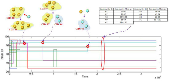
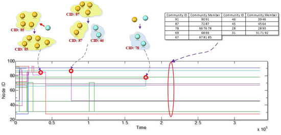
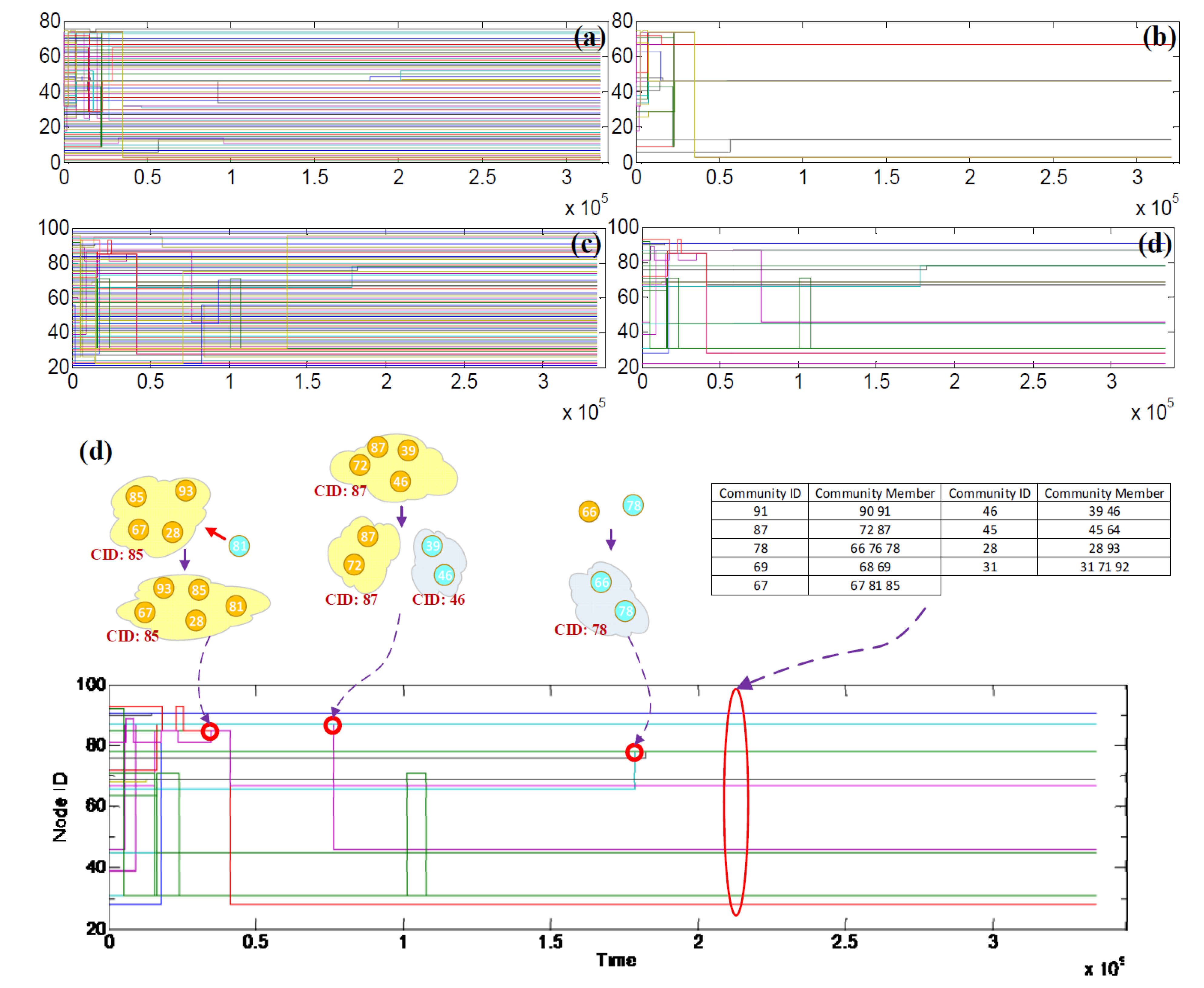
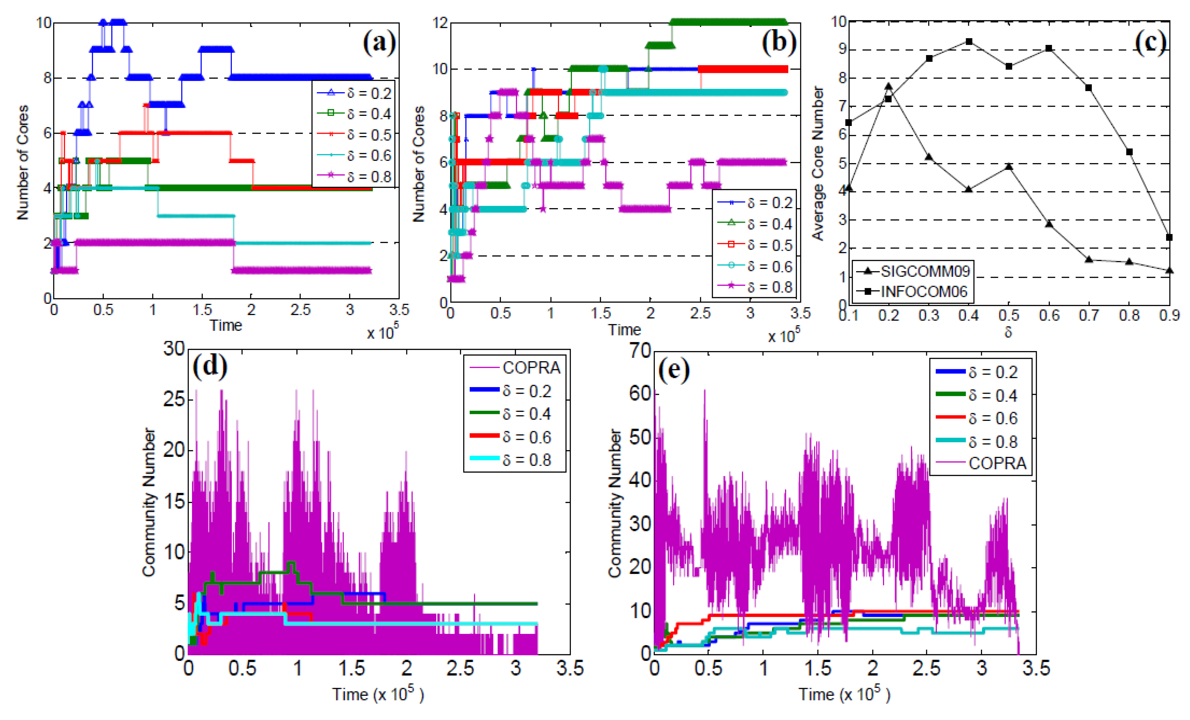
5.4. Community Core Tracking

In this part, we focus on the visualization of community core evolution to depict the stability of community cores. Firstly, we extract the community ID of each node. If a node doesn’t belong to any core, it is labeled with its node ID. Then we get the community core at each timestamp. Finally, the ID which is labeled by only one node is removed. The community core set extracted from the two datasets is presented in Figure 12. According to the selected node and the core number under the different δ scenarios, we choose δ = 0.4 in SIGCOMM09 and δ = 0.6 in INFOCOM06 to display the evolution of community cores. In Figure 12a,c a node does not belong to any community core, so its ID will be a straight line. Besides, if a node is selected as the community core, the ID will change to the core ID. Figure 12b,d show the refined core trace, including nodes belonging to the community cores only.
Figure 12. Tracking community cores; (a) Original community core evolution in SIGCOMM09 with δ = 0.4; (b) Refined community core evolution in SIGCOMM09 with δ = 0.4; (c) Original community core evolution in INFOCOM06 with δ = 0.6; (d) Refined community core evolution in INFOCOM06 with δ = 0.6; (e) Community evolution in INFOCOM06 with δ = 0.6. A few events such as merging, splitting and birth are indicated in the picture. Meanwhile, the community core partition including community IDs and community members can be tracked.
Entropy 15 05419 g012

5.5. Number of Communities

Firstly, let’s consider the variation of community cores, which is the basis of our detected communities. As shown in Figure 13, the variation of the core matrix remains at a low level. As δ increases, few changes will occur. This is due to the more stable relationship among nodes extracted by the cumulative stable contact.
Figure 13. Number of changes in core matrix between two consecutive timestamps. Above: number of changes in SIGCOMM09 under δ = 0.2, 0.4, 0.6, 0.8 (from left to right). Below: number of changes in INFOCOM06 under δ = 0.2, 0.4, 0.6, 0.8 (from left to right).
Entropy 15 05419 g013
As depicted in Figure 14a,b, after about 2 × 10⁵ seconds, the community count under each different case become fixed, which is same as the selected nodes. However, the core number in INFOCOM06 is more complicated. Like the variation of selected nodes, the number of community cores fluctuates as time changes (Figure 14a).
As mentioned before, this is due to the frequent contact among strangers. In other words, attendees at SIGCOMM09 have a more fixed social circle than at INFOCOM06. The last but most important feature of the community core count is that the core number does not change monotonically with the changes. We can see in Figure 14c, the maximum average core count (≈ 7.71) in SIGCOMM09 appears when δ = 0.2. After a reduction to δ = 0.4, the average core count rises to approximately 4.87 when δ = 0.5. The same phenomenon appears in INFOCOM06, where the core count reaches the max value at δ = 0.4 (≈ 9.31). Then it declines to approximately 8.4 at δ = 0.5, and grows to approximately 9.05 at δ = 0.6. The reason for this situation can be explained from two sides. On the one hand, the higher will filter out more contacts, which fragments the mobile network more and increases the number of community cores. On the other hand, some network fragments with low contact frequency will be moved out of the community core set entirely, which result in a reduction of the number of cores. Hence, the number of cores fluctuates under the different scenarios.
Figure 14d,e depict the comparison of community number using two datasets. The community number in SIGCOMM09 is dramatically changed. Because the contact information is less than in INFOCOM06, there are no links in a few of the timestamps. Hence, there are no communities detected by COPRA, which leads to the empty partition. Moreover, the variation of community number using CoCE is smaller than with COPRA.
Figure 14. Number of community cores. (a) Variation of community core number in SIGCOMM09; (b) variation about community core number in INFOCOM06; (c) average number of community cores in the two datasets with different δ values; (d) number of communities in SIGCOMM09; (e) number of communities in INFOCOM06.
Entropy 15 05419 g014

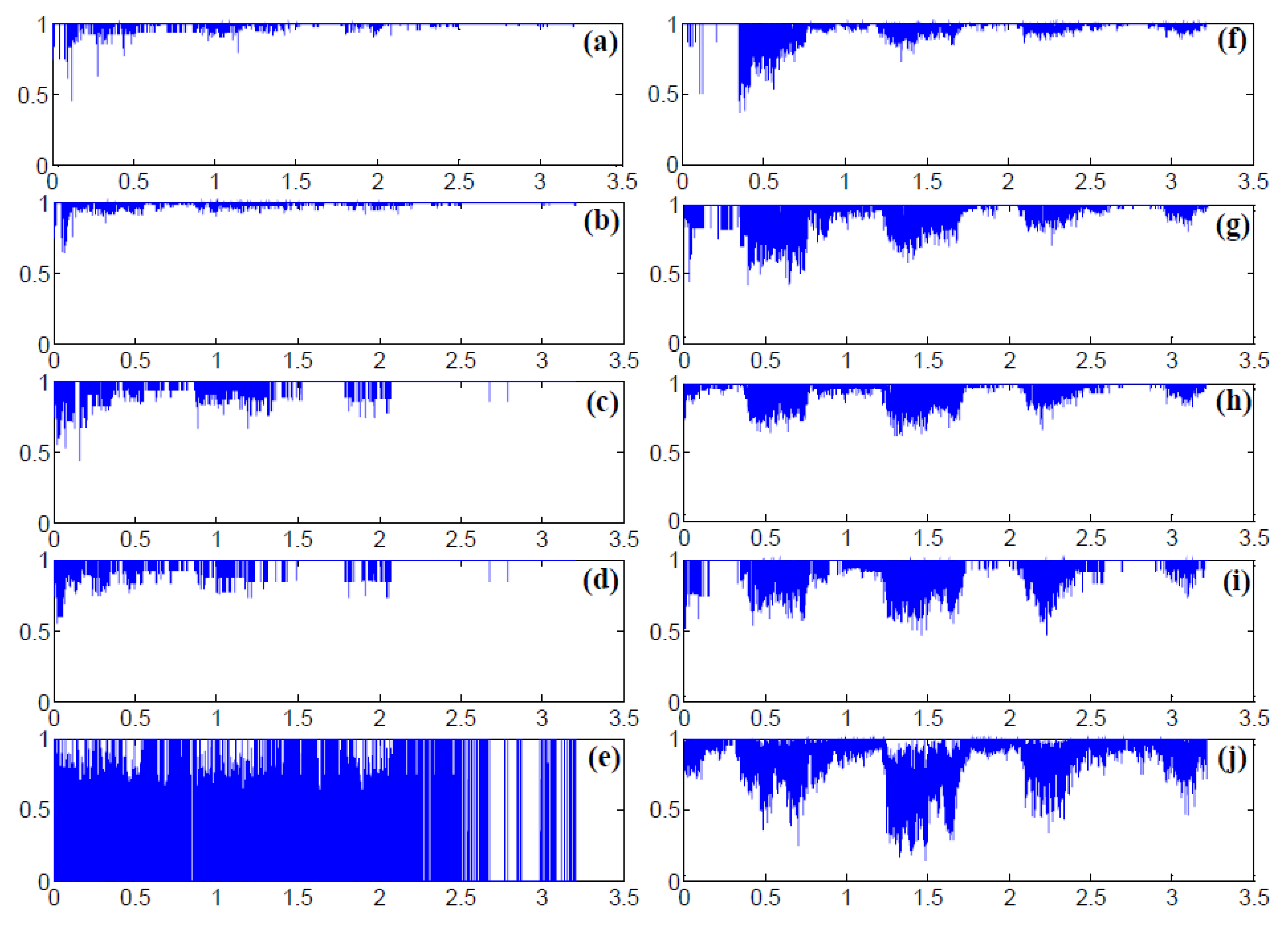
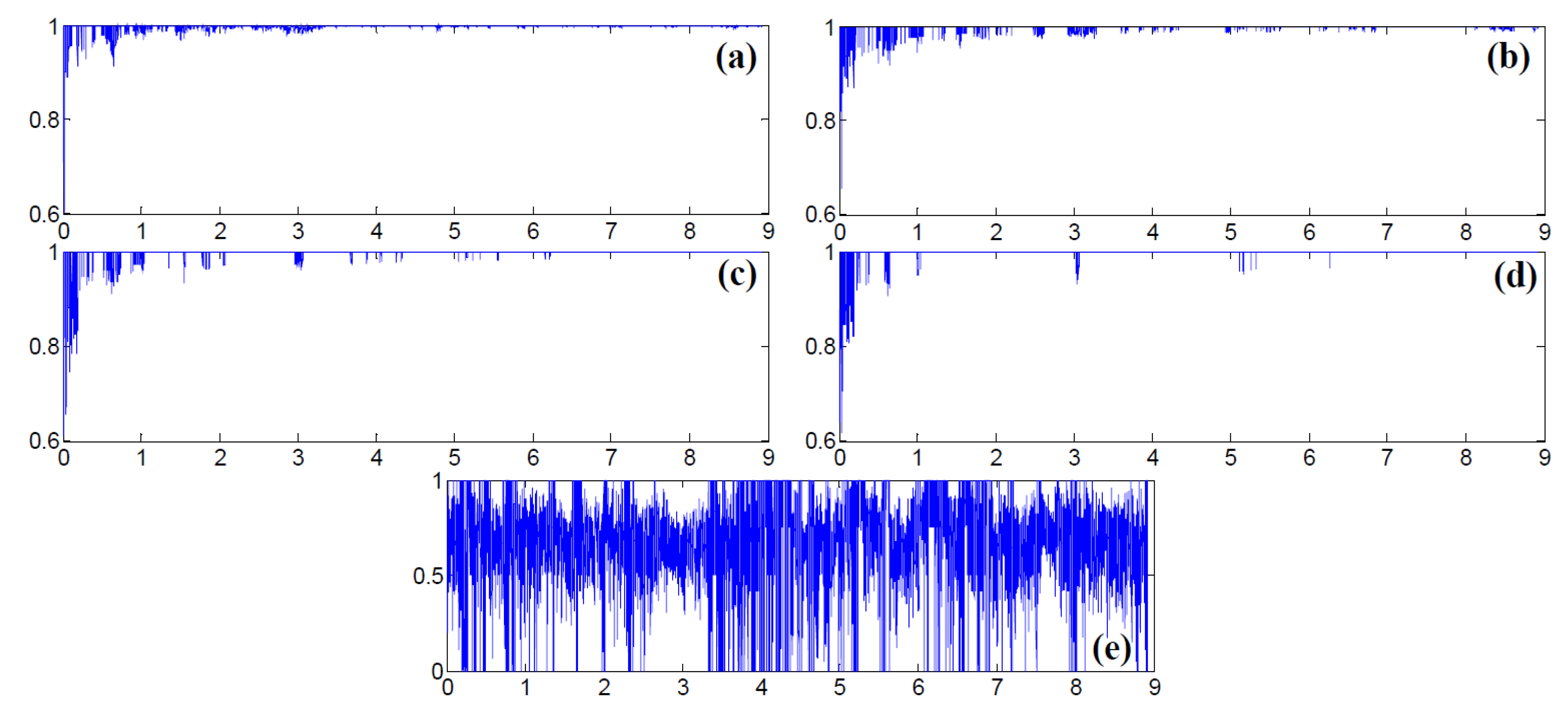
5.6. Normalized Mutual Information
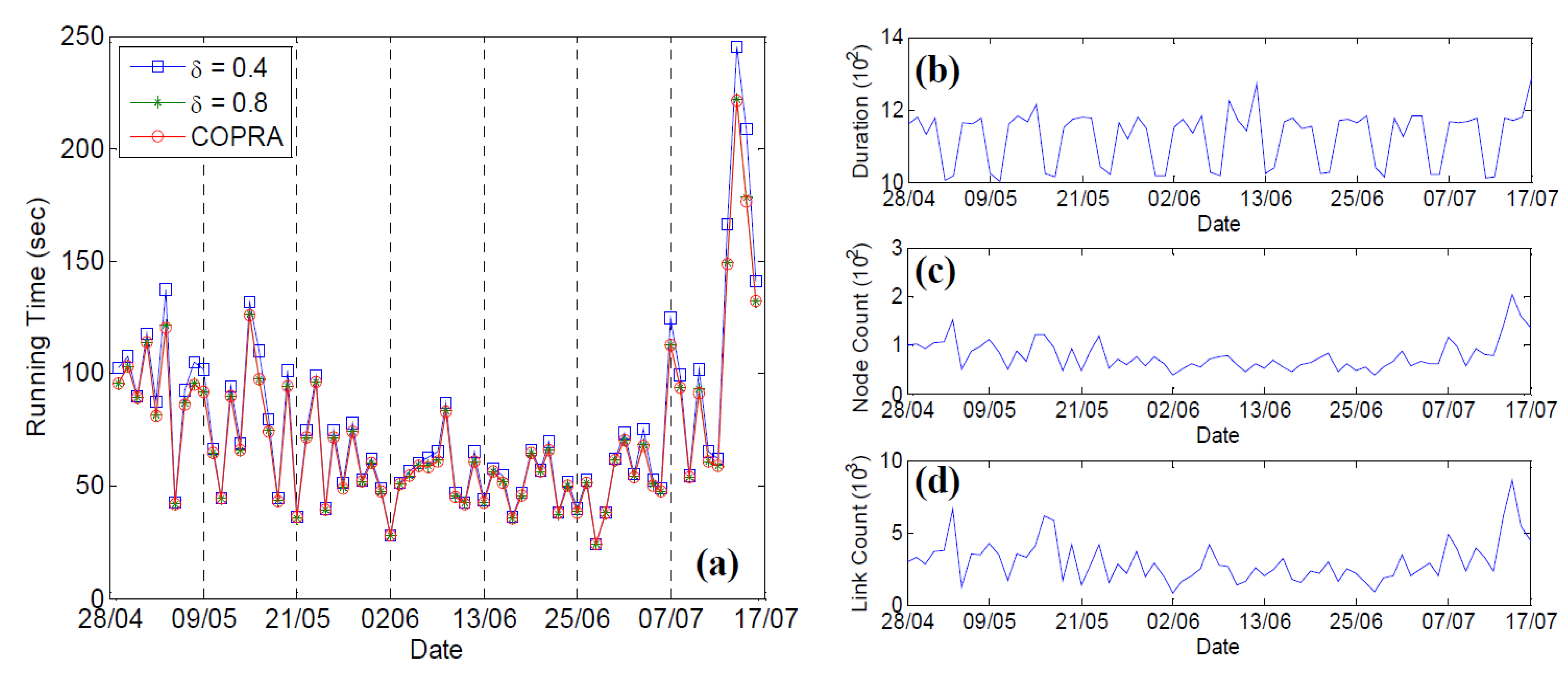
In order to quantify the stability of the identified community structure, we adapt the Normalized Mutual Information (NMI) [28] to denote the similarity between two community partitions. NMI is a reliable measurement which can be used in evaluating community detection algorithms [29]. We use COPRA for our comparison experiment.
Figure 15 depicts that the NMI value of communities detected by CoCE is higher than COPRA, which means that number of communities detected by CoCE is more stable than with COPRA. With increasing δ, a few nodes will be clustered as community core nodes, and many nodes become non-core nodes. Hence, although CoCE detects communities based on the stable community cores, the topology of communities is sensitive to the temporary links, which causes the variation of NMI value. Furthermore, an interesting observation can be made about the NMI values computed from SIGCOMM09 by COPRA. The NMI values are changing dramatically between consecutive timestamps. According to the discusseion above, there are no links in a few of timestamps in SIGCOMM09. Hence, there are no communities detected by COPRA, which uses temporary links. This phenomenon also demonstrates that the CoCE is more suitable for detecting the stable communities in dynamic networks.
Figure 15. NMI comparison between CoCE and COPRA. (ad) the NMI score computed by CoCE from δ = 0.2, 0.4, 0.6, 0.8 (SIGCOMM09); (e) the NMI score computed by COPRA in SIGCOMM09; (f–i) the NMI score computed by CoCE from δ = 0.2, 0.4, 0.6, 0.8 (INFOCOM06); (j) the NMI score computed by COPRA in INFOCOM06.
Entropy 15 05419 g015

5.7. Scalability

Besides the datasets which contain only no more than 100 nodes, we have validated the availability of CoCE in a larger dataset. INFECTIOUS contains the daily dynamic contact networks collected during the Infectious SocioPatterns event that took place at the Science Gallery in Dublin, Ireland [30]. From 28th April to 17th July, all contact information was recorded, including 10,972 nodes and 415,912 contacts. The contact interval is 20 seconds.
In this section, contacts from 1st May to 10th May are adopted. Figure 16 depicts the NMI value of communities detected by CoCE and COPRA. From Figure 16a–d, as time goes on, it can be seen that NMI scores increase as well, which means that the communities detected by CoCE are more and more stable. Moreover, as it shows that in SIGCOMM09 and INFOCOM06, few of nodes will be selected to be community core nodes with increasing δ. This will result in an increase of the non-core nodes. However, different from SIGCOMM09 and INFOCOM06, nodes in INFECTIOUS are uncertain on different days, and have high population mobility. In other words, a large proportion of nodes will change each day, while in SIGCOMM09 and INFOCOM06, people are in the conference region and their activity ranges are relatively fixed. Hence, the difference of nodes’ contact frequency between different days in INFECTIOUS are small, and the selected core nodes are insensitive to the changes of δ. It can be seen that there is no big difference among Figure 16a–d.
Figure 16. NMI comparison between CoCE and COPRA. INFECTIOUS. X-axis: timestamps, 103; Y-axis: NMI score. (ad) the NMI score computed by CoCE from δ = 0.2, 0.4, 0.6, 0.8; (e) the NMI score computed by COPRA.
Entropy 15 05419 g016
Comparing the experimental results between CoCE and COPRA, the NMI value of communities detected by CoCE is higher than with COPRA. Furthermore, in the large scale social networks, communities detected by CoCE are also more stable than with COPRA as shown in SIGCOMM09 and INFOCOM06.
Running time is an important factor in performance evaluation, especially in large scale social networks. COPRA is a very fast community detection algorithm. Figure 17 depicts the running time of CoCE and COPRA. In order to understand the performance of the algorithms, the collection duration of each day is shown in Figure 17b, as well as the node count and link count in each day (Figure 17c, d).
Figure 17. Running time of CoCE and COPRA in INFECTIOUS. (a) Comparison between CoCE and COPRA; (b) the collecting duration of each day; (c) the node count in each day; (d) the link count in each day.
Entropy 15 05419 g017
Figure 17b reveals a periodic collection time variation. There are about 1,200 sampling timestamps per day from Monday to Friday, and then it is reduced to about 1,000 per day on the weekend. Due to the cyclic feature of the collection time, the number of nodes and links each day reveal the periodic variation as well. The node and link count on normal days are higher than on the weekend. It is interesting that the number of collected nodes on Monday is higher than on other days.
The running times of CoCE and COPRA are depicted in Figure 17a. On the one hand, the running times of both algorithms are influenced by the number of nodes and links. Comparing Figure 17a,c and d, the running time will increase with the increasing number of nodes and links, and vice versa. On the other hand, the running time of CoCE in δ = 0.4 and 0.8 are similar to COPRA, which means that our algorithm performs as well as COPRA in running time.

6. Conclusions

In this paper, a dynamic community detection algorithm in mobile social networks is proposed. Firstly, the change of cumulative stable contact is discussed. We find this change follows the power-law distribution, and then propose the CoCE algorithm to extract communities from two experimental mobile social networks. Finally, we introduce a label-based community tracking algorithm, which can briefly display the evolution of communities. Based on the community cores extracted through cumulative contact histories, the communities detected by CoCE are much more stable than existing algorithms, including the number of communities and NMI. Moreover, the stable community partition is less influenced by the temporal topologies of the network than in existing methods. Furthermore, based on the experiment scalability results, we show that the communities extracted by CoCE are stable and can be further used in network analysis in large mobile social networks.

Conflict of Interest

The authors declare no conflict of interest.

Acknowledgments

This project is being jointly supported in part by the National Natural Science Foundation of China under Grant Nos. 61302144 and 61303062.

References

  1. Zhang, Y.; Yeung, D-.Y. Overlapping Community Detection via Bounded Nonnegative Matrix Tri-factorization. In Proceedings of the ACM SIGKDD International Conference on Knowledge Discovery and Data Mining, Beijing, China, 12–16 August 2012; pp. 606–614.
  2. Lin, W.; Kong, X.; Yu, P.S.; Wu, Q.; Jia, Y.; Li, C. Community Detection in Incomplete Information Networks. In Proceedings of International Conference on World Wide Web (WWW), Lyon, France, 16–20 April 2012; pp. 341–350.
  3. Bródka, P.; Saganowski, S.; Kazienko, P. Group Evolution Discovery in Social Networks. In Proceedings of the International Conference on Advances in Social Networks Analysis and Mining (ASONAM), Kaohsiung, Taiwan, 25–27 July 2011; pp. 247–253.
  4. Cazabet, R.; Amblard, F.; Hanachi, C. Detection of Overlapping Communities in Dynamical Social Networks. In Proceedings of IEEE International Conference on Social Computing (SocialCom), Minneapolis, MN, USA, 20–22 August 2010; pp. 309–314.
  5. Seifi, M.; Guillaume, J.-L. Community Cores in Evolving Networks. In Proceedings of International Conference companion on World Wide Web (MSND), Lyon, France, 16–20 April 2012.
  6. Hui, P.; Crowcroft, J.; Diot, C.; Gass, R.; Scott, J. Impact of human mobility on opportunistic forwarding algorithms. IEEE Trans. Mobile Comput. 2007, 6, 606–620. [Google Scholar]
  7. Nguyen, N.P.; Dinh, T.N.; Xuan, Y.; Thai, M.T. Adaptive Algorithms for Detecting Community Structure in Dynamic Social Networks. In Proceedings of the IEEE Conference on Computer Communications (INFOCOM), Shanghai, China, 10–15 April 2011; pp. 2282–2290.
  8. Hui, P. People are the Network: Experimental Design and Evaluation of Social-Based Forwarding Algorithms. Technical Report UCAM-CL-TR-713; University of Cambridge Computer Laboratory: Cambridge, UK, 2008. [Google Scholar]
  9. Xu, H.; Xiao, W.; Tang, D.; Tang, J.; Wang, Z. Community core evolution in mobile social networks. Sci. World J. 2013, 2013, 781281. [Google Scholar] [CrossRef] [PubMed]
  10. Holme, P.; Saramaki, J. Temporal Networks. Phys. Rep. 2012, 519, 97–125. [Google Scholar] [CrossRef]
  11. Chakrabarti, D.; Kumar, R.; Tomkins, A. Evolutionary Clustering. In Proceedings of 12th ACM SIGKDD International Conference on Knowledge Discovery and Data Mining, Philadelphia, Pennsylvania, PA, USA, 20–23 August 2006.
  12. Kim, M.-S.; Han, J. A Particle-and-Density Clustering Method for Dynamic Networks. In Proceedings of VLDB, Lyon, France, 24–28 August 2009.
  13. Chi, Y.; Song, X.; Zhou, D.; Hino, K.; Tseng, B.L. Evolutionary Spectral Clustering by Incorporating Temporal Smoothness. In Proceedings of 13th ACM SIGKDD International Conference on Knowledge Discovery and Data Mining, San Jose, CA, USA, 12–15 August 2007.
  14. Yang, T.; Chi, Y.; Zhu, S.; Gong, Y.; Rong, J. Detecting communities and their evolutions in dynamic social networks—a Bayesian approach. Mach. Learn. 2011, 82, 157–189. [Google Scholar] [CrossRef]
  15. Tang, X.; Yang, C.C. Dynamic Community Detection with Temporal Dirichlet Process. In Proceedings of 3rd International Conference on Social Computing (SocialCom), Boston, MA, USA, 9–11 October 2011.
  16. Lin, Y.-R.; Chi, Y.; Zhu, S.; Sundaram, H.; Tseng, B.L. FacetNet: A Framework for Analyzing Communities and Their Evolutions in Dynamic Networks. In Proceedings of the 23rd International World Wide Web Conference, Beijing, China, 21–25 April 2008.
  17. Nguyen, N.P.; Dinh, T.N.; Tokala, S.; Thai, M.T. Overlapping Communities in Dynamic Networks: Their Detection and Mobile Applications. In Proceedings of the 17th Annual International Conference on Mobile Computing and Networking (MobiCom), Las Vegas, CA, USA, 19–23 September 2011.
  18. Hui, P.; Yoneki, E.; Chan, S.-Y.; Crowcroft, J. Distributed Community Detection in Delay Tolerant Networks. In Proceedings of 2nd ACM/IEEE International Workshop on Mobility in the Evolving Internet Architecture (MobiArch), Kyoto, Japan, 27 August 2007.
  19. Chan, S.-Y.; Hui, P.; Xu, K. Community Detection of Time-Varying Mobile Social Networks. In Proceedings of The 1st International Conference on Complex Sciences: Theory and Applications (Complex), Shanghai, China, 23–25 February 2009.
  20. Greene, D.; Doyle, D.; Cunningham, P. Tracking the Evolution of Communities in Dynamic Social Networks. In Proceedings of International Conference on Advances in Social Networks Analysis and Mining (ASONAM), Odense, Denmark, 9–11 August 2010.
  21. Bródka, P.; Saganowski, S.; Kazienko, P. Group Evolution Discovery in Social Networks. In Proceedings of International Conference on Advances in Social Networks Analysis and Mining (ASONAM), Kaohsiung, Taiwan, 25–27 July 2011.
  22. Pietiläinen, A.-K.; Oliver, E.; LeBrun, J.; Varghese, G.; Diot, C. MobiClique: Middleware for Mobile Social Networking. In Proceedings of the 2nd ACM Workshop on Online Social Networks (WOSN), Barcelona, Spain, 17 August 2009; pp. 49–54.
  23. Wang, D.; Pedreschi, D.; Song, C.; Giannotti, F.; Barabási, A.-L. Human Mobility, Social Ties, and Link Prediction. In Proceedings of 17th ACM SIGKDD International Conference on Knowledge Discovery and Data Mining, San Diego, CA, USA, 21–24 August 2011.
  24. Bródka, P.; Saganowski, S.; Kazienko, P. GED: The method for group evolution discovery in social networks. Soc. Netw. Anal. Min. 2013, 3, 1–14. [Google Scholar] [CrossRef]
  25. Gliwa, B.; Bródka, P.; Zygmunt, A.; Saganowski, S.; Kazienko, P.; Koźlak, J. Different Approaches to Community Evolution Prediction in Blogosphere. In Proceedings of SNAA 2013 at ASONAM, Niagara Falls, Canada, 25–28 August 2013.
  26. Gliwa, B.; Saganowski, S.; Zygmunt, A.; Bródka, P.; Kazienko, P.; Koźlak, J. Identification of Group Changes in Blogosphere. In Proceedings of International Conference on Advances in Social Networks Analysis and Mining (ASONAM), Istanbul, Turkey, 26–29 August 2012.
  27. Gregory, S. Finding overlapping communities in networks by label propagation. New J. Phys. 2011, 12, 103018. [Google Scholar] [CrossRef]
  28. Meila, M. Comparing clusterings—An information based distance. J. Multivar. Anal. 2007, 98, 873–895. [Google Scholar] [CrossRef]
  29. Lancichinetti, A.; Fortunato, S.; Kertesz, J. Detecting the overlapping and hierarchical community structure in complex networks. New J. Phys. 2009, 11, 033015. [Google Scholar] [CrossRef]
  30. Isella, L.; Stehle, J.; Barrat, A.; Cattuto, C.; Pinton, J.-F.; vanden Broeck, W. What’s in a crowd? Analysis of face-to-face behavioral networks. J. Theor. Biol. 2011, 271, 166–180. [Google Scholar] [CrossRef] [PubMed] [Green Version]

