Consistency and Generalization Bounds for Maximum Entropy Density Estimation

Abstract

We investigate the statistical properties of maximum entropy density estimation, both for the complete data case and the incomplete data case. We show that under certain assumptions, the generalization error can be bounded in terms of the complexity of the underlying feature functions. This allows us to establish the universal consistency of maximum entropy density estimation.

1. Introduction

The maximum entropy (ME) principle, originally proposed by Jaynes in 1957 [1], is an effective method for combining different sources of evidence from complex, yet structured, natural systems. It has since been widely applied in science, engineering and economics. In machine learning, ME was first popularized by Della Pietra et al. [2], who applied it to induce overlapping features for a Markov random field model of natural language. Later, it was applied to other machine learning areas, such as information fusion [3] and reinforcement learning [4]. It is now well known that for complete data, the ME principle is equivalent to maximum likelihood estimation (MLE) in a Markov random field. In fact, these two problems are exact duals of one another. Recently, Wang et al. [5] proposed the latent maximum entropy (LME) principle to extend Jaynes’ maximum entropy principle to deal with hidden variables, and demonstrated its effectiveness in many statistical models, such as mixture models, Boltzmann machines and language models [6]. We show that LME is different from both Jaynes’ maximum entropy principle and maximum likelihood estimation, but it often yields better estimates in the presence of hidden variables and limited training data. This paper investigates the statistical properties of maximum entropy density estimation for both the complete and incomplete data cases.

Large sample asymptotic convergence results for MLE are typically based on point estimation analysis [7] in parametric models. Although point estimators have been extensively studied in the statistics literature since Fisher, these analyses typically do not consider generalization ability. Vapnik and Chervonenkis famously reformulated the problem of MLE for density estimation in the framework of empirical risk minimization and provided the first necessary and sufficient conditions for consistency [8,9]. However, the model they considered is still in a Fisher–Wald parametric setting. Barron and Sheu [10] considered a density estimation problem very similar to the one we address here, but only restricted to the one-dimensional case within a bounded interval. Their analysis cannot be easily generalized to a high dimensional case. Recently, Dudik et al. [11] analyzed regularized maximum entropy density estimation with inequality constraints and derived generalization bounds for this model. However, once again, their analysis does not easily extend beyond the specific model considered.

Some researchers have studied the consistency of maximum likelihood estimators under the Hellinger divergence [12], which is a particularly convenient measure for studying maximum likelihood estimation in a general distribution-free setting. However, Kullback–Leibler divergence is a more natural measure for probability distributions and is closely related to the perplexity measure used in language modeling and speech recognition research [13,14]. Moreover, convergence in the Kullback–Leibler divergence always establishes consistency in terms of Hellinger divergence [12], but not vice versa. Therefore, we concentrate on using the Kullback–Leibler divergence in our analysis.

In this paper, we investigate consistency and generalization bounds for maximum entropy density estimation with respect to the Kullback–Leibler divergence. The main technique we use in our analysis is Rademacher complexity, first used by Koltchinskii and Panchenko [15] to analyze the generalization error of combined classification methods, such as boosting, support vector machines and neural networks. Since then, the convenience of Rademacher analysis has been exploited by many to analyze various learning problems in classification and regression. For example, Rakhlin et al. [16] have used this technique to derive risk bounds for the density estimation of mixture models, which basically belong to directed graphical models using a conditional parameterization. Here, we use the Rademacher technique to analyze the generalization error of maximum entropy density estimation for general Markov random fields.

2. Maximum Entropy Density Estimation: Complete Data

Let $X\in \mathcal{X}$ be a random variable. Given a set of feature functions $\mathcal{F}\left(x\right)=\{f_1\left(x\right),...,f_N\left(x\right)\}$ specifying properties one would like to match in the data, the maximum entropy principle states that we should select a probability model, $p\left(x\right)$, from the space of all probability distributions, $\mathcal{P}\left(x\right)$, over $\mathcal{X}$, to maximize entropy subject to the constraint that the feature expectations are preserved:

$$\begin{array}{c}\hfill \underset{p\left(x\right)\in \mathcal{P}\left(x\right)}{max}\left[-{\int }_{x\in \mathcal{X}}p\left(x\right)logp\left(x\right)\mu \left(dx\right)\right]\end{array}$$

(1)

$$\begin{array}{ccc}\hfill \mathrm{s}.\mathrm{t}.{\int }_{x\in \mathcal{X}}{f}_i\left(x\right)p\left(x\right)\mu \left(dx\right)& =& {\int }_{x\in \mathcal{X}}{f}_i\left(x\right)p_0\left(x\right)\mu \left(dx\right);i=1...N,\hfill \end{array}$$

(2)

where $p_0\left(x\right)$ denotes the unknown underlying true density and μ denotes a given σ-finite measure on $\mathcal{X}$. If $\mathcal{X}$ is finite or countably infinite, then μ is the counting measure, and integrals reduce to sums. If $\mathcal{X}$ is a subset of a finite dimensional space, μ is the Lebesgue measure. If $\mathcal{X}$ is a combination of both cases, μ will be a combination of both measures. The dual problem is:

$$\begin{array}{c}\hfill \underset{\lambda \in \Omega }{min}\left[-{\int }_{x\in \mathcal{X}}{p}_0\left(x\right)log{p}_{\lambda }\left(x\right)\mu \left(dx\right)\right]\end{array}$$

(3)

where $p_{\lambda }\left(x\right)={\Phi }_{\lambda }^{-1}exp\left({\sum }_{i=1}^N{\lambda }_i{f}_i\left(x\right)\right)$ and ${\Phi }_{\lambda }={\int }_{x\in \mathcal{X}}exp\left({\sum }_{i=1}^N{\lambda }_i{f}_i\left(x\right)\right)\mu \left(dx\right)$ is a normalizing constant that ensures ${\int }_{x\in \mathcal{X}}{p}_{\lambda }\left(x\right)\mu \left(dx\right)=1$.

We will use the following notation and terminology throughout the analysis below. Define:

$$\Omega =\left\{\lambda \in {\Re }^N:{\int }_{x\in \mathcal{X}}exp\left(\sum _{i=1}^N{\lambda }_i{f}_i\left(x\right)\right)\mu \left(dx\right)<\infty \right\}$$

and let:

$$\mathcal{E}\left(x\right)=\left\{p_{\lambda }\left(x\right)\in \mathcal{P}\left(x\right):p_{\lambda }\left(x\right)=\frac{1}{{\Phi }_{\lambda }}exp\left(\sum _{i=1}^N{\lambda }_i{f}_i\left(x\right)\right),\lambda \in \Omega \right\}$$

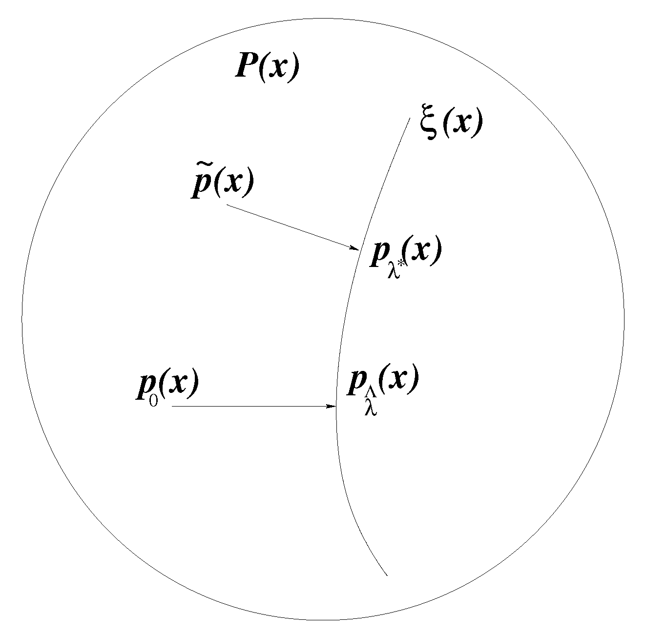
denote the exponential family induced by the set of feature functions. The restriction, $\lambda \in \Omega$, will guarantee that the maximum likelihood estimate is an interior point of the set of λ’s for which $p_{\lambda }\left(x\right)$ is defined. The optimal solution, $p_{\widehat{\lambda }}\left(x\right)$, of Equation (1) or Equation (3) is called the information projection [10,17] of $p_0\left(x\right)$ to the exponential family, $\mathcal{E}\left(x\right)$.

In practice, the true distribution, $p_0\left(x\right)$, is not known, but instead, a collection of data $\tilde{\mathcal{X}}=(x_1,\cdots ,x_M)$ sampled from $p_0\left(x\right)$ is given. Therefore, instead of using the true distribution, $p_0\left(x\right)$, we use the empirical distribution, $\tilde{p}\left(x\right)$, to calculate the feature expectations. The ME principle then becomes:

$$\begin{array}{c}\hfill \underset{p\left(x\right)\in \mathcal{P}}{max}\left[-{\int }_{x\in \mathcal{X}}p\left(x\right)logp\left(x\right)\mu \left(dx\right)\right]\end{array}$$

(4)

$$\begin{array}{ccc}\hfill \mathrm{s}.\mathrm{t}.{\int }_{x\in \mathcal{X}}{f}_i\left(x\right)p\left(x\right)\mu \left(dx\right)& =& \sum _{x\in \tilde{\mathcal{X}}}\tilde{p}\left(x\right)f_i\left(x\right);i=1...N,\hfill \end{array}$$

(5)

and the dual problem using these constraints becomes:

$$\begin{array}{c}\hfill \underset{\lambda \in \Omega }{min}\left[-\frac{1}{M}\sum _{j=1}^{M}log{p}_{\lambda }\left(x_j\right)\right]\end{array}$$

(6)

The optimal solution, $p_{{\lambda }^{*}}\left(x\right)$, of Equation (4) or Equation (6) is the information projection of $\tilde{p}\left(x\right)$ to the exponential family, $\mathcal{E}\left(x\right)$; see Figure 1.

Figure 1. In the space of all probability distributions, $\mathcal{P}\left(x\right)$ over $\mathcal{X}$, $p_{\widehat{\lambda }}\left(x\right)$ is the information projection of the true (but unknown) distribution, $p_0\left(x\right)$, to the exponential family, $\mathcal{E}$, and $p_{{\lambda }^{*}}\left(x\right)$ is the information projection of the empirical distribution, $\tilde{p}\left(x\right)$, to $\mathcal{E}$.

Figure 1. In the space of all probability distributions, $\mathcal{P}\left(x\right)$ over $\mathcal{X}$, $p_{\widehat{\lambda }}\left(x\right)$ is the information projection of the true (but unknown) distribution, $p_0\left(x\right)$, to the exponential family, $\mathcal{E}$, and $p_{{\lambda }^{*}}\left(x\right)$ is the information projection of the empirical distribution, $\tilde{p}\left(x\right)$, to $\mathcal{E}$.

2.1. Consistency and Generalization Bounds of Estimation Error

There are two standard ways to measure the quality of the estimate, $p_{{\lambda }^{*}}\left(x\right)$.

One approach, based on the Kullback–Leibler divergence, was first considered by Barron and Sheu [10]. Basically, it uses the following well-known Pythagorean property (see Lemma 3 in [10]):

$$\begin{array}{ccc}\hfill D\left(p_0\left(x\right)\parallel p_{\lambda }\left(x\right)\right)& =& D\left(p_0\left(x\right)\parallel p_{\widehat{\lambda }}\left(x\right)\right)+D\left(p_{\widehat{\lambda }}\left(x\right)\parallel p_{\lambda }\left(x\right)\right)\forall p_{\lambda }\left(x\right)\in \mathcal{E}\hfill \end{array}$$

(7)

and, in particular, the decomposition:

$$\begin{array}{ccc}\hfill D\left(p_0\left(x\right)\parallel p_{{\lambda }^{*}}\left(x\right)\right)& =& D\left(p_0\left(x\right)\parallel p_{\widehat{\lambda }}\left(x\right)\right)+D\left(p_{\widehat{\lambda }}\left(x\right)\parallel p_{{\lambda }^{*}}\left(x\right)\right)\hfill \end{array}$$

(8)

Here, the first term, $D(p_0\left(x\right)\parallel p_{\widehat{\lambda }}\left(x\right))$, is the approximation error introduced by the bias of the set of feature functions, $\mathcal{F}$, which measures how closely the feature functions are able to approximate the true probability distribution. The second term, $D(p_{\widehat{\lambda }}\left(x\right)\parallel p_{{\lambda }^{*}}\left(x\right))$, is the estimation error for densities in the exponential family, introduced by the variance of using a finite sample size. These two terms resemble the bias-variance tradeoff in least squares cost estimation [18]. The approximation error always exists unless the set of feature functions, $\mathcal{F}$, is rich enough [19]. In this paper, we assume that the set of feature functions is given and study how close $p_{\widehat{\lambda }}\left(x\right)$ is to $p_{{\lambda }^{*}}\left(x\right)$.

Another way to evaluate the quality of $p_{{\lambda }^{*}}\left(x\right)$ is to measure the difference between the best expected likelihood and the empirical likelihood of the estimate, which is a more desirable approach, because we can directly calculate the empirical likelihood of the estimate from the training data.

Both approaches, in fact, fall under the umbrella of Vapnik’s empirical risk minimization principle [8] for density estimation. Here, we use the first approach to show that the maximum entropy solution converges to the best possible solution, $p_{\widehat{\lambda }}\left(x\right)$, and the second approach to show that the value of empirical likelihood converges to the maximum expected likelihood.

2.1.1. Maximum Entropy Principle

Exploiting tools from empirical process theory, including symmetrization, concentration and contraction inequalities, Koltchinskii and Panchenko [15] were able to give bounds on the generalization error of boosting, support vector machines (SVMs) and neural networks. We show through the following theorem that we can use similar tools to establish generalization bounds for the estimation error of maximum entropy density estimation. All proofs can be found in the Appendix.

Theorem 1. 

Assuming ${sup}_{\lambda \in \Omega }{\parallel \lambda \parallel }_1<\infty$ and ${sup}_{f\in \mathcal{F},x\in \mathcal{X}}{\parallel f\left(x\right)\parallel }_{\infty }<\infty$, then there exist $0<\zeta <\alpha <\infty$, such that, for any $\eta \in (0,1)$, with a probability of at least $1-\eta$,

$$\begin{array}{ccc}\hfill D(p_{\widehat{\lambda }}\left(x\right)\parallel p_{{\lambda }^{*}}\left(x\right))& =& D(p_0\left(x\right)\parallel p_{{\lambda }^{*}}\left(x\right))-D(p_0\left(x\right)\parallel p_{\widehat{\lambda }}\left(x\right))\hfill \\ & \le & \frac{4C_1}{\sqrt{M}}{E}_{\tilde{\mathcal{X}}}\left[{\int }_{\zeta }^{\alpha }\sqrt{log\mathcal{N}(\mathcal{F}\left(x\right),ϵ,d_x)}dϵ\right]+C_2\sqrt{\frac{2log\left(\frac{1}{\eta }\right)}{M}}\hfill \end{array}$$

(9)

where M is the number of instances, $\mathcal{N}(\mathcal{F}\left(x\right),ϵ,d_x)$ is the random covering number [20,21] for linear combinations of functions in $\mathcal{F}\left(x\right)$ at scale ϵ with empirical Euclidean distance $d_x$ on sample $\tilde{\mathcal{X}}$, and $C_1$ and $C_2$ are positive constants that do not depend on the instance.

If the linear combination of feature functions belongs to a VC-subgraph with Vapnik-Chervonenkis (VC) dimension V, it is well known that the Dudley integral is bounded by $\sqrt{V}$ [12,20,22].

Rakhlin et al. [16] first applied a similar technique to derive generalization bounds for the density estimation of mixture models. Here, we apply the technique to derive bounds for maximum entropy density estimation in general Markov random fields. Even though the analysis we use is standard, our results show that the generalization bound is not related to the log partition function, but instead is upper bounded by the covering number of linear combinations of feature functions. This is an important observation, because the log partition function—a fundamental quantity associated with any graph-structured distribution—is NP-hard to compute in general [23].

Although the assumption that ${sup}_{f\in \mathcal{F},x\in \mathcal{X}}{\parallel f\left(x\right)\parallel }_{\infty }<\infty$ seems rather restrictive, most of the graphical models studied in machine learning [23] are, in fact, discrete Markov random fields, which always satisfy this condition.

To eliminate the assumption of boundedness on the parameters and feature functions, we use a result adapted from [24].

Theorem 2. 

Assume that there exists a positive number, $K\left(\mathcal{F}\right)$, such that for all $\tau >0$,

$$\begin{array}{c}\hfill log{E}_{p_0\left(x\right)}\left(p_{{\lambda }^{•}}{\left(x\right)}^{2\tau }-\frac{1}{p_{{\lambda }^{•}}{\left(x\right)}^{2\tau }}\right)\le (\tau K\left(\mathcal{F}\right){)}^2\end{array}$$

(10)

where ${\lambda }^{•}$ are parameters, such that $E_{p_{{\lambda }^{•}}\left(x\right)}\left(f\left(x\right)\right)=f\left(x\right)$. Then, for all $\lambda \in \Omega$, we have, with a probability of at least $1-\eta$,

$$\begin{array}{ccc}& & E_{p_0\left(x\right)}log{p}_{\lambda }\left(x\right)-\frac{1}{M}\sum _{j=1}^{M}log{p}_{\lambda }\left(x_j\right)\hfill \\ & \le & E_{\tilde{\mathcal{X}}}\underset{\lambda \in \Omega ,f\left(x\right)\in \mathcal{F}\left(x\right)}{sup}(E_{p_0\left(x\right)}\langle \lambda ,f\left(x\right)\rangle -E_{\tilde{p}\left(x\right)}\langle \lambda ,f\left(x\right)\rangle )+K\left(\mathcal{F}\right)\sqrt{\frac{2log\left(\frac{1}{\eta }\right)}{M}}\hfill \end{array}$$

(11)

By the above result, Theorem 1 can be proven by replacing $C_2$ with $K\left(\mathcal{F}\right)$. Since the value, $K\left(\mathcal{F}\right)$, is hard to determine in practice, we state our results in terms of the bound on feature functions instead. Nevertheless, the reader should keep in mind that this bound can be replaced by $K\left(\mathcal{F}\right)$ in all our results.

Using the result of [21], the following theorem gives a useful bound on the covering number.

Theorem 3. 

Assume ${sup}_{\lambda \in \Omega }{\parallel \lambda \parallel }_2<a$ and ${sup}_{f\in \mathcal{F},x\in \mathcal{X}}{\parallel f\left(x\right)\parallel }_2<b$, then:

$$\begin{array}{ccc}& & {log}_2\mathcal{N}(\mathcal{F}\left(x\right),ϵ,d_x)\le \lceil \frac{a^2{b}^2}{{ϵ}^2}\rceil (min\left({log}_2(2M+1),{log}_2(2N+1)\right))\hfill \end{array}$$

(12)

We then have the following corollaries. The first is a direct consequence of Theorem 1. The second provides a generalization bound on the expected value of the estimation error, which can be shown using the proof in [16,20].

Corollary 1. 

Universal consistency: If ${\int }_{\zeta }^{\alpha }\sqrt{log\mathcal{N}(\mathcal{F}\left(x\right),ϵ,d_x)}dϵ$ is bounded, then as $M\to \infty$, $p_{{\lambda }^{*}}\left(x\right)$ will converge to $p_{\widehat{\lambda }}\left(x\right)$ in terms of the Kullback–Leibler divergence with rate $\mathcal{O}(\frac{1}{\sqrt{M}})$, independent of the form of the true distribution, $p_0$.

Corollary 2. 

Under the conditions of Theorem 1, the generalization bound of the expected estimation error is:

$$\begin{array}{ccc}\hfill E_{\tilde{\mathcal{X}}}D(p_{\widehat{\lambda }}\left(x\right)\parallel p_{{\lambda }^{*}}\left(x\right))& =& E_{\tilde{\mathcal{X}}}D(p_0\left(x\right)\parallel p_{{\lambda }^{*}}\left(x\right))-D(p_0\left(x\right)\parallel p_{\widehat{\lambda }}\left(x\right))\hfill \\ & \le & \frac{4C_1}{\sqrt{M}}{E}_{\tilde{\mathcal{X}}}\left[{\int }_{\zeta }^{\alpha }\sqrt{log\mathcal{N}(\mathcal{F}\left(x\right),ϵ,d_x)}dϵ\right]+\frac{C_2^2}{M}\hfill \end{array}$$

(13)

Next, we turn to the second approach to evaluating the quality of $p_{{\lambda }^{*}}\left(x\right)$; namely, by measuring the difference between the expected log-likelihood and the empirical log-likelihood. This is the approach used by Dudik et al. [11].

Define ${\mathcal{L}}_0\left(\lambda \right)=-{\int }_{x\in \mathcal{X}}{p}_0\left(x\right)log{p}_{\lambda }\left(x\right)\mu \left(dx\right)$ and $\tilde{\mathcal{L}}\left(\lambda \right)=-\frac{1}{M}{\sum }_{j=1}^{M}log{p}_{\lambda }\left(x_j\right)$. Then, from Theorem 1 and the McDiarmid concentration inequality, we obtain the following result for the sample log-likelihood, which is similar to Dudik et al. [11].

Theorem 4. 

There are $0<\zeta <\alpha <\infty$, such that, with a probability of at least $1-\eta$:

$$\begin{array}{ccc}\hfill |{\mathcal{L}}_0\left(\widehat{\lambda }\right)-\tilde{\mathcal{L}}\left({\lambda }^{*}\right)|& =& |E_{p_0\left(x\right)}log{p}_{\widehat{\lambda }}\left(x\right)-\frac{1}{M}\sum _{j=1}^{M}log{p}_{{\lambda }^{*}}\left(x_j\right)|\hfill \\ & \le & \frac{6C_1}{\sqrt{M}}{E}_{\tilde{\mathcal{X}}}\left[{\int }_{\zeta }^{\alpha }\sqrt{log\mathcal{N}(\mathcal{F}\left(x\right),ϵ,d_x)}dϵ\right]+3C_2\sqrt{\frac{log\left(\frac{1}{\eta }\right)}{2M}}\hfill \end{array}$$

(14)

By the Glivenko–Cantelli theorem [9], we know that the empirical distribution converges to the true distribution. Therefore, under certain conditions, the entropy of empirical distribution will also converge to the entropy of the true distribution. Whenever such convergence holds, we can combine this with Theorem 3 to show that $D(p_0\left(x\right)\parallel p_{\widehat{\lambda }}\left(x\right))-D(\tilde{p}\left(x\right)\parallel p_{{\lambda }^{*}}\left(x\right))\to 0$ as $M\to \infty$, establishing a stronger form of consistency than Corollary 1.

2.1.2. Regularized Maximum Entropy Principle

In many statistical modeling settings, the constraints used in the ME principle are subject to errors from the empirical nature of the data. This is particularly true in domains with sparse, high dimensional data. One way to gain robustness, though, is to relax the constraints and add a penalty to the entropy, leading to the regularized ME (RME) principle [25]:

$$\underset{p\left(x\right),\mathbf{a}}{max}\left[-{\int }_{x\in \mathcal{X}}p\left(x\right)logp\left(x\right)\mu \left(dx\right)-U\left(\mathbf{a}\right)\right]$$

(15)

$$\mathrm{s}.\mathrm{t}.{\int }_{x\in \mathcal{X}}p\left(x\right)f_i\left(x\right)\mu \left(dx\right)=\sum _x\tilde{p}\left(x\right)f_i\left(x\right)+a_i;i=1,...,N$$

(16)

Here, $\mathbf{a}={(a_1,...,a_N)}^T$, $a_i$ is the error for each constraint, and $U:{\Re }^N\to \Re$ is a cost function that has a value of zero at zero. The function penalizes any constraint violations, and can be used to penalize deviations in the more reliably observed constraints to a greater degree than deviations in less reliably observed constraints.

The dual problem of RME becomes:

$$\begin{array}{c}\hfill \underset{\lambda \in \Omega }{min}\left[-\frac{1}{M}\sum _{j=1}^{M}log{p}_{\lambda }\left(x_j\right)+U^{*}\left(\lambda \right)\right]\end{array}$$

(17)

which is equivalent to maximum a posteriori (MAP) estimation with prior $U^{*}\left(\lambda \right)$. Note that the prior, $U^{*}\left(\lambda \right)$, is derived from the penalty function, U, over errors $\mathbf{a}$, by setting $U^{*}$ to the convex (Fenchel) conjugate [26,27] of U, i.e., $U^{*}\left(\lambda \right)={sup}_{\mathbf{a}}\langle \lambda ,\mathbf{a}\rangle -U\left(\mathbf{a}\right)$. This function is always convex, regardless of the convexity of U. Conversely, given the convex conjugate cost function, $U^{*}$, the corresponding penalty function, U, can be derived by using the property of Fenchel biconjugation [26]; that is, the conjugate of the conjugate of a convex function is the original convex function, $U=U^{**}$.

Conventionally, $U\left(\mathbf{a}\right)$ is chosen to be nonnegative and have a minimum of zero at zero. To illustrate, consider a quadratic penalty $U\left(\mathbf{a}\right)={\sum }_{i=1}^N\frac{1}{2}{\sigma }_i^2{a}_i^2$. Here, the convex conjugate $U^{*}\left(\lambda \right)={\sum }_{i=1}^N\frac{{\lambda }_i^2}{2{\sigma }_i^2}$ can be determined by setting $a_i=\frac{{\lambda }_i}{{\sigma }_i^2}$, which specifies a Gaussian prior on λ. A different example can be obtained by considering the Laplacian prior on λ, $U^{*}\left(\lambda \right)={\parallel \lambda \parallel }_1={\sum }_{i=1}^N\left|{\lambda }_i\right|$, which leads to the penalty function:

$$U\left(\mathbf{a}\right)=\left\{\begin{array}{c}{0\parallel \mathbf{a}\parallel }_{\infty }=\underset{i=1}{\overset{N}{max}}\left|a_i\right|\le 1\hfill \\ \infty \text{otherwise}\hfill \end{array}\right.$$

that forces hard inequality constraints.

However, there is an important aspect of the validity of choosing a legal (log) prior, $U^{*}$, which has been ignored in previous studies on the RME principle [11,25,28,29]. To see this, consider the following. By plugging the true distribution, $p_0\left(x\right)$, instead of the empirical distribution into Equation (16), one obtains:

$$\underset{p\left(x\right),\mathbf{a}}{max}\left[-{\int }_{x\in \mathcal{X}}p\left(x\right)logp\left(x\right)\mu \left(dx\right)-U\left(\mathbf{a}\right)\right]$$

(18)

$$\mathrm{s}.\mathrm{t}.{\int }_{x\in \mathcal{X}}p\left(x\right)f_i\left(x\right)\mu \left(dx\right)={\int }_{x\in \mathcal{X}}{p}_0\left(x\right)f_i\left(x\right)+a_i;i=1,...,N$$

(19)

The dual problem is:

$$\begin{array}{c}\hfill \underset{\lambda \in \Omega }{min}\left[-{\int }_{x\in \mathcal{X}}{p}_0\left(x\right)log{p}_{\lambda }\left(x\right)+U^{*}\left(\lambda \right)\right]\end{array}$$

(20)

Since $p_{\widehat{\lambda }}\left(x\right)$ is the information projection of $p_0\left(x\right)$ to the exponential family, $\mathcal{E}\left(x\right)$, we must have $U\left(\widehat{\mathbf{a}}\right)=U^{*}(\widehat{\lambda })=0$ and $\widehat{\mathbf{a}}=0$, where $\widehat{\mathbf{a}}$ denotes the $\mathbf{a}$ corresponding to $\widehat{\lambda }$. Moreover, as a penalty term, the prior, $U^{*}\left(\lambda \right)$, should be nonnegative with a minimum of zero. We call the prior satisfying these conditions a legal prior. Both the standard Gaussian prior $U^{*}\left(\lambda \right)={\sum }_{i=1}^N\frac{{\lambda }_i^2}{2{\sigma }_i^2}$ and standard Laplacian prior $U^{*}\left(\lambda \right)={\parallel \lambda \parallel }_1$ do not satisfy $U^{*}(\widehat{\lambda })=0$. The correct choices for these priors should be $U^{*}(\lambda -\widehat{\lambda })={\sum }_{i=1}^N\frac{{({\lambda }_i-{\widehat{\lambda }}_i)}^2}{2{\sigma }_i^2}$ for a Gaussian prior and $U^{*}(\lambda -\widehat{\lambda })={\parallel \lambda -\widehat{\lambda }\parallel }_1$ for a Laplacian prior, respectively. Consequently, $U\left(\mathbf{a}\right)$ should be chosen as $U\left(\mathbf{a}\right)+\langle \mathbf{a},\widehat{\lambda }\rangle$. Note that $U\left(\mathbf{a}\right)+\langle \mathbf{a},\widehat{\lambda }\rangle$ does have a value of zero at zero, but it is no longer nonnegative.

If we let $p_{{\lambda }^{▵}}$ denote the solution to Equation (17), we then obtain the following generalization bound on estimation error without any restrictions on $U\left(\mathbf{a}\right)$ or $U^{*}\left(\lambda \right)$.

Theorem 5. 

Assume ${sup}_{\lambda \in \Omega }{\parallel \lambda \parallel }_1<\infty$ and ${sup}_{f\in \mathcal{F},x\in \mathcal{X}}{\parallel f\left(x\right)\parallel }_{\infty }<\infty$. Then, there exist $0<\zeta <\alpha <\infty$, such that with a probability of at least $1-\eta$,

$$\begin{array}{ccc}\hfill D(p_{\widehat{\lambda }}\left(x\right)\parallel p_{{\lambda }^{▵}}\left(x\right))& =& D(p_0\left(x\right)\parallel p_{{\lambda }^{▵}}\left(x\right))-D(p_0\left(x\right)\parallel p_{\widehat{\lambda }}\left(x\right))\hfill \\ & \le & \frac{4C_1}{\sqrt{M}}{E}_{\tilde{\mathcal{X}}}\left[{\int }_{\zeta }^{\alpha }\sqrt{log\mathcal{N}(\mathcal{F}\left(x\right),ϵ,d_x)}dϵ\right]+C_2\sqrt{\frac{2log\left(\frac{1}{\eta }\right)}{M}}\hfill \\ & & +U^{*}\left(\widehat{\lambda }\right)-U^{*}\left({\lambda }^{▵}\right)\hfill \end{array}$$

(21)

We then have the following result that guarantees the universal consistency of RME.

Corollary 3. 

Universal consistency: If ${\int }_{\zeta }^{\alpha }\sqrt{log\mathcal{N}(\mathcal{F}\left(x\right),ϵ,d_x)}dϵ$ is bounded and $U^{*}(\widehat{\lambda })\le U^{*}\left({\lambda }^{▵}\right)$, then as $M\to \infty$, $p_{{\lambda }^{▵}}\left(x\right)$ will converge to $p_{\widehat{\lambda }}\left(x\right)$ in terms of their Kullback–Leibler divergence with rate $O\left(\frac{1}{\sqrt{M}}\right)$, for any true distribution, $p_0\left(x\right)$, and prior distribution.

If we choose $U^{*}\left(\lambda \right)$ to be a legal prior, then we also have a further result.

Corollary 4. 

Assume ${sup}_{\lambda \in \Omega }{\parallel \lambda \parallel }_1<\infty$, ${sup}_{f\in \mathcal{F},x\in \mathcal{X}}{\parallel f\left(x\right)\parallel }_{\infty }<\infty$ and that $U^{*}\left(\lambda \right)$ is a legal prior. Then, there exist $0<\zeta <\alpha <\infty$, such that, with a probability of at least $1-\eta$,

$$\begin{array}{ccc}\hfill D(p_{\widehat{\lambda }}\left(x\right)\parallel p_{{\lambda }^{▵}}\left(x\right))& =& D(p_0\left(x\right)\parallel p_{{\lambda }^{▵}}\left(x\right))-D(p_0\left(x\right)\parallel p_{\widehat{\lambda }}\left(x\right))\hfill \\ & & \le \frac{4C_1}{\sqrt{M}}{E}_{\tilde{\mathcal{X}}}\left[{\int }_{\zeta }^{\alpha }\sqrt{log\mathcal{N}(\mathcal{F}\left(x\right),ϵ,d_x)}dϵ\right]+C_2\sqrt{\frac{2log\left(\frac{1}{\eta }\right)}{M}}-U^{*}\left({\lambda }^{▵}\right)\hfill \end{array}$$

(22)

Moreover, as $M\to \infty$, both $U^{*}\left({\lambda }^{▵}\right)\to 0$ and $p_{{\lambda }^{▵}}\left(x\right)$ will converge to $p_{\widehat{\lambda }}\left(x\right)$ in terms of their Kullback–Leibler divergence with rate $O(\frac{1}{\sqrt{M}})$, for any true distribution, $p_0\left(x\right)$, and prior distribution.

The legal prior guarantees RME’s consistency without introducing any regularization parameter, as commonly done in machine learning [9,19]. Since $U^{*}\left({\lambda }^{▵}\right)\ge 0$ for any legal prior, this result shows that RME always obtains a lower generalization bound than ME, even without assuming the truth of the prior.

Using the result of Theorem 5 and the McDiarmid concentration inequality, we are able to derive a generalization bound on the difference between the best expected log-likelihood and the log of the MAP probability. This holds for any regularization cost function, as long as $U^{*}\left(\widehat{\lambda }\right)\le U^{*}\left({\lambda }^{▵}\right)$, without requiring that $U^{*}\left(\lambda \right)$ be convex. We note that Dudik et al. [11] gave a similar result, but only for the special case of using the $l_1$ norm as a penalty in the dual formulation; see Equation (17).

For a broad family of regularization functions, i.e., log priors in Equation (17), such that the Hessian matrices of λ (the prior information matrices) are positive definite, we can improve the convergence rate from $\mathcal{O}\left(\frac{1}{\sqrt{M}}\right)$ to $\mathcal{O}\left(\frac{1}{M}\right)$. The techniques needed to prove the $\mathcal{O}\left(\frac{1}{M}\right)$ convergence rate were first proposed by Zhang [19,30,31] to show the consistency and generalization bounds of various classification methods based on convex risk optimization with the $l_2$-penalty.

Define the convex function:

$$\begin{array}{c}\hfill L_{\lambda }\left(x\right)=-log{p}_{\lambda }\left(x\right)=-log\frac{exp(\langle \lambda ,f(x)\rangle )}{{\int }_{x^{\prime }}exp\left(\langle \lambda ,f\left(x^{\prime }\right)\rangle \right)\mu \left(d{x}^{\prime }\right)}=log{\int }_{x^{\prime }}exp\left(\langle \lambda ,f\left(x^{\prime }\right)-f\left(x\right)\rangle \right)\mu \left(d{x}^{\prime }\right)\end{array}$$

(23)

Consider training samples ${\tilde{\mathcal{X}}}_{M+1}=(x_1,\cdots ,x_{M+1})$. Let $\tilde{\lambda }$ be the solution of Equation (24) with training data ${\tilde{\mathcal{X}}}_{M+1}$.

$$\begin{array}{c}\hfill \underset{\lambda \in \Omega }{min}\left[\frac{1}{M}\sum _{j=1}^{M+1}{L}_{\lambda }\left(x_j\right)+U^{*}\left(\lambda \right)\right]\end{array}$$

(24)

Let ${\tilde{\lambda }}_k$ be the solution of Equation (24) with training sample $x_k$ removed from the set, ${\tilde{\mathcal{X}}}_{M+1}$. We have the following lemma that extends the quadratic case considered in [19,31]. We prove the result in its full generality, though our proof is essentially a variant of the stability results by Zhang [19,30,31].

Lemma 1. 

Assume the Hessian matrix of $U^{*}\left(\lambda \right)$ is positive definite with smallest eigenvalue κ. Then, $\parallel \tilde{\lambda }-{\tilde{\lambda }}_k{\parallel }_2\le \frac{2}{\kappa M}|\nabla L_{\tilde{\lambda }}\left(x_k\right)|$.

Finally, we can obtain the following leave-one-out error bound, which has a convergence rate of $\mathcal{O}\left(\frac{1}{M}\right)$.

Theorem 6. 

Let $C={sup}_{x,x^{\prime }}\parallel f\left(x\right)-f\left(x^{\prime }\right)\parallel$. When the legal prior, $U\left(\lambda \right)$, is chosen, such that its Hessian matrix of λ is positive definite with smallest eigenvalue κ, the expected generalization error can then be bounded as:

$$\begin{array}{ccc}\hfill E_{\tilde{\mathcal{X}}}D(p_{\widehat{\lambda }}\left(x\right)\parallel p_{{\lambda }^{▵}}\left(x\right))& =& E_{\tilde{\mathcal{X}}}D(p_0\left(x\right)\parallel p_{{\lambda }^{▵}}\left(x\right))-D(p_0\left(x\right)\parallel p_{\widehat{\lambda }}\left(x\right))\hfill \\ & \le & \frac{C^2}{\kappa M}(1-exp(-E_X{L}_{\widehat{\lambda }}\left(X\right))\hfill \end{array}$$

(25)

3. Maximum Entropy Density Estimation: Incomplete Data

Here, we consider a variable to be “latent” or “hidden” if it is never observed, but causally effects the observations [6]. In practice, many of the natural patterns we wish to classify are the result of causal processes that have a hidden hierarchical structure, yielding data that does not report the value of latent variables [6]. Obtaining fully labeled data is tedious or impossible in many realistic cases. This motivates us to propose an unsupervised statistical learning technique, the latent maximum entropy (LME) principle, which is still formulated in terms of maximizing entropy, except that we must now change the problem formulation to respect hidden variables.

Following the terminology of the expectation-maximization (EM) algorithm [6], let $Y\in \mathcal{Y}$ be the observed incomplete data, $Z\in \mathcal{Z}$ be the missing data and then $X=(Y,Z)\in \mathcal{X}$ be the random variable denoting the complete data That is, $X=(Y,Z)$. For example, Y might be observed natural language in the form of text and Z might be its missing syntactic and semantic information. If we let $p\left(x\right)$ and $p\left(y\right)$ denote the densities of X and Y, respectively, and let $p\left(z\right|y)$ denote the conditional density of Z given Y, then $p\left(y\right)={\int }_{z\in \mathcal{Z}}p\left(x\right)\mu \left(dz\right)$, and $p\left(x\right)=p\left(y\right)p\left(z\right|y)$. The LME principle can be stated as follows.

Given features $f_1\left(x\right),...,f_N\left(x\right)$, specifying the properties that we would like to match in the data, select a joint probability model, $p\left(x\right)$, from the space of all probability distributions, $\mathcal{P}\left(x\right)$, over $\mathcal{X}$, to maximize the entropy:

$$\begin{array}{c}\hfill \underset{p\left(x\right)\in \mathcal{P}}{max}\left[-{\int }_{x\in \mathcal{X}}p\left(x\right)logp\left(x\right)\mu \left(dx\right)\right]\end{array}$$

(26)

$$\begin{array}{ccc}\hfill \mathrm{s}.\mathrm{t}.{\int }_{x\in \mathcal{X}}{f}_i\left(x\right)p\left(x\right)\mu \left(dx\right)& =& \sum _{y\in \tilde{\mathcal{Y}}}\tilde{p}\left(y\right){\int }_{z\in \mathcal{Z}}{f}_i\left(x\right)p\left(z\right|y)\mu \left(dz\right),i=1,...,N\hfill \end{array}$$

(27)

where $x=(y,z)$ and $\tilde{p}\left(y\right)$ is the empirical distribution of the observed data, $\tilde{\mathcal{Y}}=(y_1,\cdots ,y_M)$ denotes the set of observed Y values and $p\left(z\right|y)$ is the conditional distribution of latent variables given the observed data. Intuitively, the constraints specify that we require the expectations of $f_i\left(X\right)$ in the joint model to match their empirical expectations on the incomplete data, Y, taking into account the structure of the implied dependence of the unobserved component, Z, on Y.

Note that the conditional distribution, $p\left(z\right|y)$, implicitly encodes the latent structure and is a nonlinear mapping of $p\left(x\right)$. That is, $p\left(z\right|y)=\frac{p(y,z)}{{\int }_{z^{\prime }\in \mathcal{Z}}p(y,z^{\prime })\mu \left(dz\right)}=\frac{p\left(x\right)}{{\int }_{z^{\prime }\in \mathcal{Z}}p\left(x^{\prime }\right)\mu \left(d{z}^{\prime }\right)}$, where $x=(y,z)$ and $x^{\prime }=(y,z^{\prime })$ by definition. Clearly, $p\left(z\right|y)$ is a nonlinear function of $p\left(x\right)$ because of the division.

Unfortunately, there is no simple optimal solution for $p\left(x\right)$ in Equation (26) and Equation (27). However, a good approximation can be obtained by restricting the model to $p_{\lambda }\left(x\right)={\Phi }_{\lambda }^{-1}exp\left({\sum }_{i=1}^N{\lambda }_i{f}_i\left(x\right)\right)$ where ${\Phi }_{\lambda }={\int }_{x\in \mathcal{X}}exp\left({\sum }_{i=1}^N{\lambda }_i{f}_i\left(x\right)\right)\mu \left(dx\right)$ is the normalization constant. This restriction provides a free parameter, ${\lambda }_i$, for each feature function, $f_i\left(x\right)$. By adopting such a “log-linear” restriction, it turns out that we can formulate a practical algorithm for approximately satisfying the LME principle.

In [5], we exploited the following connection between LME and maximum likelihood estimation (MLE) to derive a practical training algorithm.

Theorem 7. 

[5] Under the log-linear assumption, maximizing the likelihood of log-linear models on incomplete data is equivalent to satisfying the feasibility constraints of the LME principle. That is, the only distinction between MLE and LME in log-linear models is that, among local maxima (feasible solutions), LME selects the model with the maximum entropy, whereas MLE selects the model with the maximum likelihood.

Define $L_{\lambda }\left(y\right))=-{\sum }_{y\in \tilde{\mathcal{Y}}}\tilde{p}\left(y\right)log{p}_{\lambda }\left(y\right)$ and $H(\lambda ,\lambda )=-{\sum }_{y\in \tilde{\mathcal{Y}}}\tilde{p}\left(y\right){\int }_{z\in \mathcal{Z}}{p}_{\lambda }\left(z\right|y)log{p}_{\lambda }\left(z\right|y)\mu \left(dz\right)$. The latter is the conditional entropy of a hidden variable over observed sample data $\tilde{\mathcal{Y}}$ that measures the uncertainty of the hidden variables. Then, in the case where λ is a feasible log-linear solution according to Equation (27), we have the following relationship between likelihood over observed data and the entropy of the joint model.

Corollary 5. 

[5] If λ is in the set of feasible solutions, then:

$$\begin{array}{c}\hfill L_{\lambda }\left(y\right)=H\left(p_{\lambda }\left(x\right)\right)-H(\lambda ,\lambda )\end{array}$$

(28)

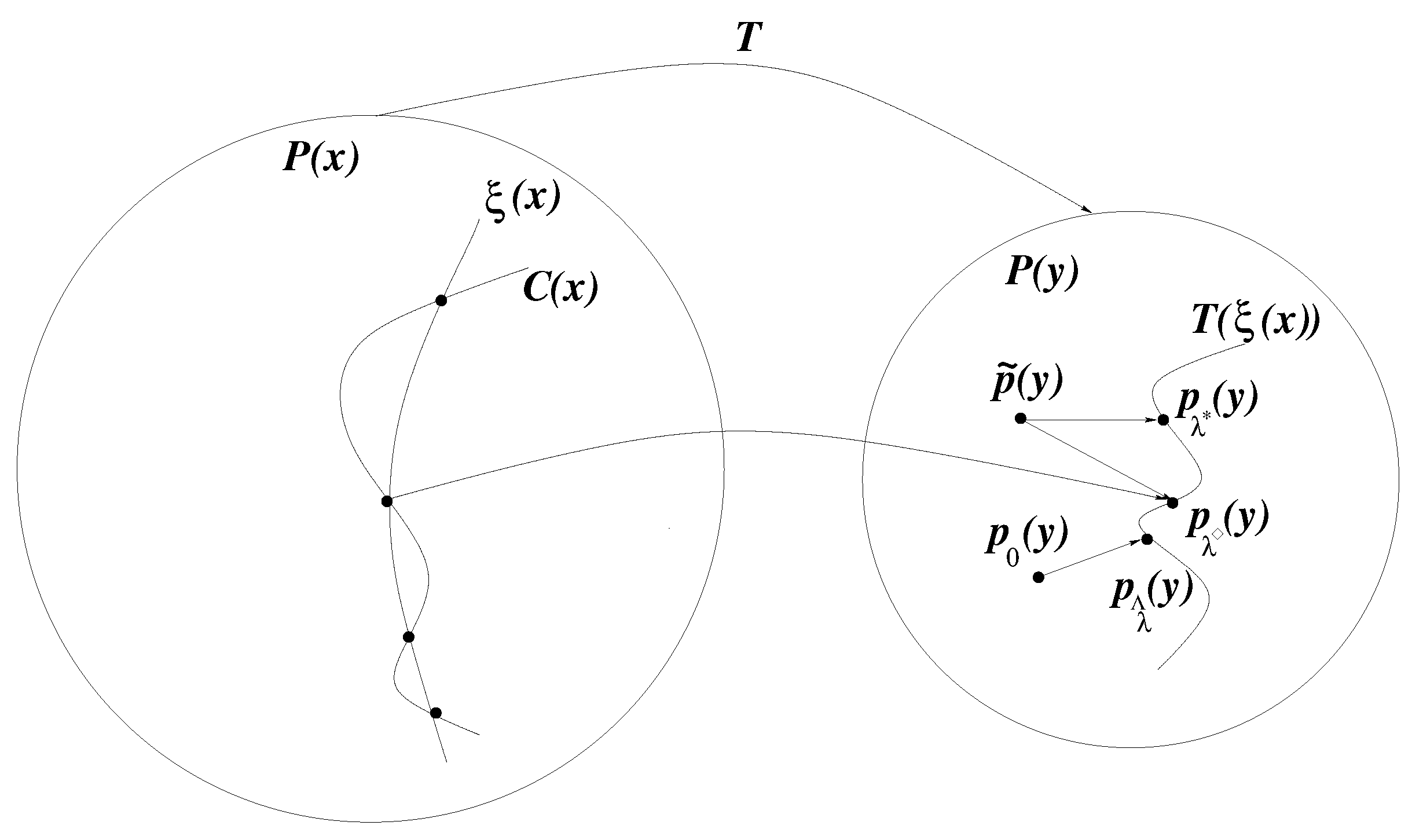
We will use the following notation and terminology throughout the analysis below. Denote the manifold of the nonlinear constraint set in Equation (27) as $\mathcal{C}$. We then define $p_{\widehat{\lambda }}\left(y\right)=arg{max}_{p_{\lambda }\left(x\right)\in \mathcal{E}}{\int }_{y\in \mathcal{Y}}{p}_0\left(y\right)log{p}_{\lambda }\left(y\right)$ as the nearest point in terms of $D\left(p_0\left(y\right)\parallel p_{\lambda }\left(y\right)\right)$ from $p_0\left(y\right)$ to the marginalized exponential family over z, using $p_{\lambda }\left(y\right)={\int }_{z\in \mathcal{Z}}{p}_{\lambda }(y,z)\mu \left(dz\right)$, where $p_{\lambda }\left(x\right)\in \mathcal{E}\left(x\right)$; see Figure 2.

Figure 2. The operator, T, denotes the marginalization of $p\left(x\right)$ over z and maps the entire space of all probability distributions, $\mathcal{P}\left(x\right)$ over $\mathcal{X}$, into the space of all probability distributions, $\mathcal{P}\left(y\right)$ over $\mathcal{Y}$. Here, $p_{\widehat{\lambda }}\left(y\right)$ is the information projection of $p_0\left(y\right)$ to the marginalized exponential family, $\mathcal{E}$; $p_{{\lambda }^{*}}\left(y\right)$ is the information projection of $\tilde{p}\left(y\right)$ to the marginalized exponential family, $\mathcal{E}$; and $p_{{\lambda }^{\diamond }}\left(y\right)$ is the distribution that in joint model space has the highest entropy among the intersection points of the exponential family, $\mathcal{E}$, and the nonlinear constraint set, $\mathcal{C}$.

Figure 2. The operator, T, denotes the marginalization of $p\left(x\right)$ over z and maps the entire space of all probability distributions, $\mathcal{P}\left(x\right)$ over $\mathcal{X}$, into the space of all probability distributions, $\mathcal{P}\left(y\right)$ over $\mathcal{Y}$. Here, $p_{\widehat{\lambda }}\left(y\right)$ is the information projection of $p_0\left(y\right)$ to the marginalized exponential family, $\mathcal{E}$; $p_{{\lambda }^{*}}\left(y\right)$ is the information projection of $\tilde{p}\left(y\right)$ to the marginalized exponential family, $\mathcal{E}$; and $p_{{\lambda }^{\diamond }}\left(y\right)$ is the distribution that in joint model space has the highest entropy among the intersection points of the exponential family, $\mathcal{E}$, and the nonlinear constraint set, $\mathcal{C}$.

In [29,32], we formulate the regularized latent maximum entropy principle (RLME) as the following:

$$\underset{p\left(x\right),\mathbf{a}}{max}\left[-{\int }_{x\in \mathcal{X}}p\left(x\right)logp\left(x\right)\mu \left(dx\right)-U\left(\mathbf{a}\right)\right]$$

(29)

subject to:

$${\int }_{x\in \mathcal{X}}p\left(x\right)f_i\left(x\right)\mu \left(dx\right)=\sum _y\tilde{p}\left(y\right){\int }_{z}p\left(z\right|y)f_i(y,z)\mu \left(dz\right)+a_i;i=1,...,N$$

(30)

Again $\mathbf{a}=(a_1,...,a_N)$, where $a_i$ is the error for each constraint, and $U:{\Re }^N\to \Re$ is a convex function with its minimum at zero.

The standard maximum a posteriori (MAP) estimate minimizes the negative penalized log-likelihood $R\left(\lambda \right)=-{\sum }_y\tilde{p}\left(y\right)log{p}_{\lambda }\left(y\right)+U^{*}\left(\lambda \right)$.

Our key result in [29,32] is that locally minimizing $R\left(\lambda \right)$ is equivalent to satisfying the feasibility constraints in Equation (30) of the RLME principle.

Theorem 8. 

[29,32] Under the log-linear assumption, locally maximizing the posterior probability of log-linear models on incomplete data is equivalent to satisfying the feasibility constraints of the RLME principle. That is, the only distinction between MAP and RLME in log-linear models is that, among local maxima (feasible solutions), RLME selects the model with the maximum regularized entropy, whereas MAP selects the model with the maximum posterior probability

Corollary 6. 

[29,32] If ${\lambda }^{*}$ is in the set of feasible solutions of Equation (30), then $R\left(\lambda \right)=H\left(p_{\lambda }\right)-U\left(\mathbf{a}\right)-H(\lambda ,\lambda )$.

3.1. Consistency and Generalization Bounds for Estimation Error

To measure the quality of the maximum likelihood and maximum entropy estimates, we do not consider the divergence of the models in the original joint space, $\mathcal{P}\left(x\right)$. Instead, we consider the marginalized models in the observed data space, $\mathcal{P}\left(y\right)$. However, to measure the divergence between models in the observed data space, we have to take the difference of $D(p_0\left(y\right)\parallel p_{{\lambda }^{*}}\left(y\right))$ and $D(p_0\left(y\right)\parallel p_{\widehat{\lambda }}\left(y\right))$, even though, technically, the Pythagorean property no longer holds in this case. Nevertheless, this still gives a useful measure of the approximation quality.

3.1.1. Maximum Likelihood Estimate

We first establish consistency and provide generalization bounds for the maximum likelihood density estimate, $p_{{\lambda }^{*}}\left(y\right)$. Note that if we attempt to use a technique similar to the complete data case here, we will obtain a bound that is governed by the covering number of the log of the marginal feature functions $\mathcal{F}\left(y\right)={\int }_{z\in \mathcal{Z}}exp\left(\langle \lambda ,f(y,z)\rangle \right)\mu \left(dz\right)$. Bounding the covering number of log-int-exp$\mathcal{F}\left(x\right)$ is more difficult than bounding it for $\mathcal{F}\left(y\right)$ directly. To cope with this issue, we use the refined version of the Rademacher comparison inequality proposed in [24] to eliminate the log function. This is a slightly different approach than that taken by Rakhlin et al. [16], who, instead, use the contraction technique of [15,20,33] to derive bounds for mixture model density estimation. Here, we pursue a streamlined analysis that avoids working with the likelihood ratio (also, see [34]),hence avoiding the second application of contraction, which results in tighter constants.

Theorem 9. 

Assume for all $\lambda \in \Omega$ and for all $y\in \mathcal{Y}$, we have $0<a\le \mathcal{F}\left(y\right)\le b$. Then, there exist $0<\zeta <\alpha <\infty$ and positive constants, $C_3,C_4\in {\Re }^{+}$, such that, with a probability of at least $1-\eta$, for any dataset of size M drawn from $p_0\left(y\right)$,

$$\begin{array}{ccc}& & D(p_0\left(y\right)\parallel p_{{\lambda }^{*}}\left(y\right))-D(p_0\left(y\right)\parallel p_{\widehat{\lambda }}\left(y\right))\hfill \\ & \le & \frac{4C_3}{\sqrt{M}}{E}_{\tilde{\mathcal{Y}}}\left[{\int }_{\zeta }^{\alpha }\sqrt{log\mathcal{N}(\mathcal{F}\left(y\right),ϵ,d_y)}dϵ\right]+C_4\sqrt{\frac{2log\left(\frac{1}{\eta }\right)}{M}}\hfill \end{array}$$

(31)

where $\mathcal{N}(\mathcal{F}\left(y\right),ϵ,d_y)$ is the random covering number of the marginal feature functions, $\mathcal{F}\left(y\right)={\int }_{z\in \mathcal{Z}}exp\left(\langle \lambda ,f(y,z)\rangle \right)\mu \left(dz\right)$, at scale ϵ with empirical Euclidean distance $d_y$ on sample data $\tilde{\mathcal{Y}}$.

Similarly, we can eliminate the assumption of boundedness on the parameters and feature functions, $\mathcal{F}\left(y\right)$, by using a result adapted from [24].

Theorem 10. 

Assume that there exists a positive number, $K\left(\mathcal{F}\right)$, such that for all $\tau >0$:

$$\begin{array}{c}\hfill log{E}_{p_0\left(y\right)}\left(p_{{\lambda }^{•}}{\left(y\right)}^{2\tau }-\frac{1}{p_{{\lambda }^{•}}{\left(y\right)}^{2\tau }}\right)\le (\tau K\left(\mathcal{F}\right){)}^2\end{array}$$

(32)

where ${\lambda }^{•}$ are the parameters $(p_{{\lambda }^{•}}{\left(y\right)}^{2\tau }-\frac{1}{p_{{\lambda }^{•}}{\left(y\right)}^{2\tau }})$ achieving the maximum subject to $E_{p_{{\lambda }^{•}}\left(x\right)}\left(f\left(x\right)\right)=E_{p_{{\lambda }^{•}}\left(z\right|y)}\left(f(y,z)\right)$. Then, for all $\lambda \in \Omega$, we have with a probability of at least $1-\eta$,

$$\begin{array}{ccc}& & E_{p_0\left(x\right)}log{p}_{\lambda }\left(y\right)-\frac{1}{M}\sum _{j=1}^{M}log{p}_{\lambda }\left(y_j\right)\hfill \\ & \le & E_{\tilde{\mathcal{Y}}}\underset{\lambda \in \Omega ,f\left(x\right)\in \mathcal{F}\left(x\right)}{sup}(E_{p_0\left(x\right)}log\mathcal{F}\left(y\right)-E_{\tilde{p}\left(x\right)}log\mathcal{F}\left(y\right))+K\left(\mathcal{F}\right)\sqrt{\frac{2log\left(\frac{1}{\eta }\right)}{M}}\hfill \end{array}$$

(33)

Using the above result, Theorem 9 can be proven by replacing $C_4$ with $K\left(\mathcal{F}\right)$. Again, since the value, $K\left(\mathcal{F}\right)$, is hard to determine in practice, we will state our results below in terms of a bound on feature functions, but as before, the reader should bear in mind that the bound on feature functions can be replaced by $K\left(\mathcal{F}\right)$.

From the results above, we can establish the following consistency property.

Corollary 7. 

Universal consistency: If ${\int }_{\zeta }^{\alpha }\sqrt{log\mathcal{N}(\mathcal{F}\left(y\right),ϵ,d_y)}dϵ$ is bounded, then $p_{{\lambda }^{*}}\left(y\right)$ will converge to $p_{\widehat{\lambda }}\left(y\right)$ (in terms of the difference of the Kullback–Leibler divergence to the true distribution, $p_0\left(y\right)$) with rate $\mathcal{O}\left(\frac{1}{\sqrt{M}}\right)$, regardless of the form of true distribution $p_0\left(y\right)$.

Similar to the complete data case, using the result of Theorem 9 and the McDiarmid concentration inequality, we are also able to derive the generalization bound for the difference of the best expected log-likelihood and the maximum empirical log-likelihood.

3.1.2. Latent Maximum Entropy Estimate

Let $p_{{\lambda }^{\diamond }}\left(y\right)$ denote the maximum entropy estimate of Equation (26) over the exponential family, $\mathcal{E}$. We use similar techniques to the case of complete data regularized maximum entropy (Section 2.1.2) to prove consistency and generalization bounds for using the latent maximum entropy density estimate, $p_{{\lambda }^{\diamond }}\left(y\right)$.

Theorem 11. 

(LME principle) Assume for all $\lambda \in \Omega$ and for all $y\in \mathcal{Y}$, we have $0<a\le \mathcal{F}\left(y\right)\le b$. Then, there exist $0<\zeta <\alpha <\infty$, such that with a probability of at least $1-\eta$,

$$\begin{array}{ccc}\hfill D(p_0\left(y\right)\parallel p_{{\lambda }^{\diamond }}\left(y\right))-D(p_0\left(y\right)\parallel p_{\widehat{\lambda }}\left(y\right))& \le & \frac{4C_3}{\sqrt{M}}{E}_{\tilde{\mathcal{Y}}}\left[{\int }_{\zeta }^{\alpha }\sqrt{log\mathcal{N}(\mathcal{F}\left(y\right),ϵ,d_y)}dϵ\right]\hfill \\ & & +C_4\sqrt{\frac{2log\left(\frac{1}{\eta }\right)}{M}}+E_{\tilde{p}\left(y\right)}log\frac{p_{\widehat{\lambda }}\left(y\right)}{p_{{\lambda }^{\diamond }}\left(y\right)}\hfill \end{array}$$

(34)

Using this result, we can then easily establish the following consistency property.

Corollary 8. 

Universal consistency: If ${\int }_{\zeta }^{\alpha }\sqrt{log\mathcal{N}(\mathcal{F}\left(y\right),ϵ,d_y)}dϵ$ is bounded and also $E_{\tilde{p}\left(y\right)}log{p}_{\widehat{\lambda }}\left(y\right)\le E_{\tilde{p}\left(y\right)}log{p}_{{\lambda }^{\diamond }}\left(y\right)$, then $p_{{\lambda }^{\diamond }}\left(y\right)$ will converge to $p_{\widehat{\lambda }}\left(y\right)$ (in terms of the difference of the Kullback–Leibler divergence to the true distribution, $p_0\left(y\right)$) with rate $\mathcal{O}\left(\frac{1}{\sqrt{M}}\right)$, for any true distribution, $p_0\left(y\right)$.

Corollary 8 gives a sufficient condition, i.e., $E_{\tilde{p}\left(y\right)}log{p}_{\widehat{\lambda }}\left(y\right)\le E_{\tilde{p}\left(y\right)}log{p}_{{\lambda }^{\diamond }}\left(y\right)$, that leads to the universal consistency of latent maximum entropy estimation. This perhaps partially explains our observations of experimental results on synthetic data conducted in [5].

Note that in the proof of Theorem 11 and Corollary 8, it is not necessary to restrict $p_{{\lambda }^{\diamond }}$ to be the model that has global maximum joint entropy over all feasible log-linear solutions. It turns out that the conclusion still holds for all feasible log-linear models, $p_{\lambda }\left(y\right)$, that have greater empirical log-likelihood, $E_{\tilde{p}\left(y\right)}log{p}_{\lambda }\left(y\right)$, than the empirical log-likelihood, $E_{\tilde{p}\left(y\right)}log{p}_{\widehat{\lambda }}\left(y\right)$, of the optimal expected log-likelihood estimate, $p_{\widehat{\lambda }}\left(y\right)$. That is, as the sample size grows, any of these feasible log-linear models will converge to $p_{\widehat{\lambda }}\left(y\right)$ (in terms of the difference of the Kullback–Leibler divergence to the true distribution, $p_0\left(y\right)$) with rate $\mathcal{O}\left(\frac{1}{\sqrt{M}}\right)$.

3.1.3. Maximum a Posteriori Estimate

In a similar manner, it is straightforward to have the following generalization bound for the MAP estimate, $p_{{\lambda }^{▵}}\left(y\right)$.

Theorem 12. 

(MAP principle) Assume for all $\lambda \in \Omega$ and for all $y\in \mathcal{Y},0<a\le \mathcal{F}\left(y\right)\le b$. Then, with a probability of at least $1-\eta$,

$$\begin{array}{ccc}& & D(p_0\left(y\right)\parallel p_{{\lambda }^{▵}}\left(y\right))-D(p_0\left(y\right)\parallel p_{{\lambda }^{▵}}\left(y\right))\hfill \\ & & \le \frac{4C_3}{\sqrt{M}}{E}_{\tilde{\mathcal{X}}}\left[{\int }_{\zeta }^{\alpha }\sqrt{log\mathcal{N}(\mathcal{F}\left(y\right),ϵ,d_x)}dϵ\right]+C_4\sqrt{\frac{2log\left(\frac{1}{\eta }\right)}{M}}+U^{*}\left(\widehat{\lambda }\right)-U^{*}\left({\lambda }^{▵}\right)\hfill \end{array}$$

(35)

By the above theorem, one can easily obtain the following consistency result.

Corollary 9. 

Universal consistency: If ${\int }_{\zeta }^{\alpha }\sqrt{log\mathcal{N}(\mathcal{F}\left(y\right),ϵ,d_y)}dϵ$ is bounded and $U^{*}\left(\widehat{\lambda }\right)\le U^{*}\left({\lambda }^{▵}\right)$, then $p_{{\lambda }^{▵}}\left(y\right)$ will converge to $p_{\widehat{\lambda }}\left(y\right)$ in terms of the difference of the Kullback–Leibler divergence to the true distribution, $p_0\left(y\right)$, with rate $\mathcal{O}\left(\frac{1}{\sqrt{M}}\right)$ without assuming the form of the true distribution, $p_0\left(y\right)$, nor the true prior distribution.

3.1.4. Regularized Latent Maximum Entropy Estimate

We can also, in a similar manner, establish the following generalization bound for the RLME estimate, $p_{{\lambda }^{\diamond }}\left(y\right)$.

Theorem 13. 

(RLME principle) Assume for all $\lambda \in \Omega$ and for all $y\in \mathcal{Y},0<a\le \mathcal{F}\left(y\right)\le b$. Then, with a probability of at least $1-\eta$,

$$\begin{array}{ccc}\hfill D(p_0\left(y\right)\parallel p_{{\lambda }^{\diamond }}\left(y\right))-D(p_0\left(y\right)\parallel p_{\widehat{\lambda }}\left(y\right))& \le & \frac{4C_3}{\sqrt{M}}{E}_{\tilde{\mathcal{X}}}\left[{\int }_{\zeta }^{\alpha }\sqrt{\mathcal{N}(\mathcal{F}\left(y\right),ϵ,d_x)}dϵ\right]+C_4\sqrt{\frac{2log\left(\frac{1}{\eta }\right)}{M}}\hfill \\ & & +E_{\tilde{p}\left(y\right)}log{p}_{\widehat{\lambda }}\left(y\right)-E_{\tilde{p}\left(y\right)}log{p}_{{\lambda }^{\diamond }}\left(y\right)+U^{*}\left(\widehat{\lambda }\right)-U^{*}\left({\lambda }^{\diamond }\right)\hfill \end{array}$$

(36)

By the above theorem, we can easily obtain the following consistency result.

Corollary 10. 

Universal consistency: If ${\int }_{\zeta }^{\alpha }\sqrt{log\mathcal{N}(\mathcal{F}\left(y\right),ϵ,d_y)}dϵ$ is bounded and $E_{\tilde{p}\left(y\right)}log{p}_{\widehat{\lambda }}\left(y\right)+U^{*}\left(\widehat{\lambda }\right)\le E_{\tilde{p}\left(y\right)}log{p}_{{\lambda }^{\diamond }}\left(y\right)+U^{*}\left({\lambda }^{\diamond }\right)$, then $p_{{\lambda }^{\diamond }}\left(y\right)$ will converge to $p_{\widehat{\lambda }}\left(y\right)$ in terms of the difference of the Kullback–Leibler divergence to the true distribution, $p_0\left(y\right)$, with rate $\mathcal{O}\left(\frac{1}{\sqrt{M}}\right)$ without assuming the form of true distribution $p_0\left(y\right)$ and true prior distribution.

4. Conclusions

We have investigated the statistical properties of using the maximum entropy principle for density estimation, in both the complete and incomplete data cases. For complete data, maximum entropy is equivalent to maximum likelihood estimation in a Markov random field. Here, we derived bounds on the generalization error based on the complexity of linear combinations of feature functions, and used this to establish a form of universal consistency. We then provided a similar analysis for regularized maximum entropy estimation, which, interestingly, yields a better generalization bound (and maintains consistency) for any legal prior. Moreover, if the information matrix of the prior is positive definite, we can further show that the convergence rate can be improved to $\mathcal{O}\left(\frac{1}{M}\right)$ instead of $\mathcal{O}\left(\frac{1}{\sqrt{M}}\right)$. For incomplete data, maximum entropy is no longer equivalent to maximum likelihood estimation, and the analysis becomes more difficult. Nevertheless, we established bounds on the generalization error of maximum likelihood in terms of the complexity of the marginalizedfeature functions, again achieving a form of universal consistency. With additional assumptions, we were able to extend this analysis to apply it to latent maximum entropy estimation and to prove its universal consistency, as well. Analogous conclusions can be drawn for regularized situations. Finally, we note that an alternative analysis can be based on replacing the Kullback–Leibler divergence with the more general Bregman distance [35,36]. The analysis here can be easily extended to this more general setting.

In our future work, we are planning to study the trade-off between approximation error and estimation error to select the best set of feature functions.

References

1. Jaynes, E. Information theory and statistical mechanics. Phys. Rev. 1957, 106, 620–630. [Google Scholar] [CrossRef]
2. Della Pietra, S.; Della Pietra, V.; Lafferty, J. Inducing features of random fields. IEEE Trans. Pattern Anal. Mach. Intell. 1997, 19, 380–393. [Google Scholar] [CrossRef]
3. Palmieri, F.; Ciuonzo, D. Objective priors from maximum entropy in data classification. Inf. Fusion 2013, 14, 186–198. [Google Scholar] [CrossRef]
4. Ziebart, B.; Maas, A.; Bagnell, J.; Dey, A. Maximum Entropy Inverse Reinforcement Learning. In Proceeding of The 23rd National Conference on Artificial Intelligence (AAAI), Chicago, IL, USA, 13–17 July 2008; pp. 1433–1438.
5. Wang, S.; Schuurmans, D.; Zhao, Y. The latent maximum entropy principle. ACM Trans. Knowl. Discov. Data 2012, 6, No. 8. 1–42. [Google Scholar] [CrossRef]
6. McLachlan, G.; Krishnan, T. The EM Algorithm and Extensions, 2nd ed.; Wiley-Interscience: Hoboken, NJ, USA, 2008. [Google Scholar]
7. Lehmann, E.L.; Casella, G. Theory of Point Estimation; Springer-Verlag: New York, NY, USA, 1998. [Google Scholar]
8. Vapnik, V.; Chervonenkis, A. The necessary and sufficient conditions for consistency in the empirical risk minimization method. Pattern Recognit. Image Anal. 1991, 1, 283–305. [Google Scholar]
9. Vapnik, V.N. Statistical Learning Theory; Wiley-Interscience: Hoboken, NJ, USA, 1998. [Google Scholar]
10. Barron, A.; Sheu, C. Approximation of density functions by sequences of exponential families. Ann. Stat. 1991, 19, 1347–1369. [Google Scholar] [CrossRef]
11. Dudik, M.; Phillips, S.; Schapire, R. Performance Guarantees for Regularized Maximum Entropy Density Estimation. In Proceedings of The 17th Annual Conference on Learning Theory (COLT), Banff, Canada, 1–4 July 2004; pp. 472–486.
12. Van de Geer, S. Empirical Processes in M-Estimation; Cambridge University Press: Cambridge, UK, 2000. [Google Scholar]
13. Jelinek, F. Statistical Methods for Speech Recognition; MIT Press: Cambridge, MA, USA, 1998. [Google Scholar]
14. Rosenfeld, R. A maximum entropy approach to adaptive statistical language modeling. Comput. Speech Lang. 1996, 10, 187–228. [Google Scholar] [CrossRef]
15. Koltchinskii, V.; Panchenko, D. Empirical margin distributions and bounding the generalization error of combined classifiers. Ann. Stat. 2002, 30, 1–50. [Google Scholar]
16. Rakhlin, A.; Panchenko, D.; Mukherjee, S. Risk bounds for mixture density estimation. ESAIM: Probab. Stat. 2005, 9, 220–229. [Google Scholar] [CrossRef]
17. Csiszar, I. I-divergence geometry of probability distributions and minimization problems. Ann. Probab. 1975, 3, 146–158. [Google Scholar] [CrossRef]
18. Barron, A. Approximation and estimation bounds for artificial neural networks. Mach. Learn. 1994, 14, 115–133. [Google Scholar] [CrossRef]
19. Zhang, T. Statistical behavior and consistency of classification methods based on convex risk minimization. Ann. Stat. 2004, 32, 56–85. [Google Scholar] [CrossRef]
20. Panchenko, D. Class Lecture Notes of MIT 18.465: Statistical Learning Theory; Massachusetts Institute of Technology: Cambridge, MA, USA, 2002. [Google Scholar]
21. Zhang, T. Covering number bounds of certain regularized linear function classes. J. Mach. Learn. Res. 2002, 2, 527–550. [Google Scholar]
22. Dudley, R. Uniform Central Limit Theorems; Cambridge University Press: New York, NY, USA, 1999. [Google Scholar]
23. Wainwright, M.; Jordan, M. Graphical models, exponential families, and variational inference. Found. Trends Mach. Learn. 2008, 1, 1–305. [Google Scholar] [CrossRef]
24. Meir, R.; Zhang, T. Generalization error bounds for Bayesian mixture algorithms. J. Mach. Learn. Res. 2003, 4, 839–860. [Google Scholar]
25. Chen, S.F.; Rosenfeld, R. A survey of smoothing techniques for ME models. IEEE Trans. Speech Audio Process. 2000, 8, 37–50. [Google Scholar] [CrossRef]
26. Borwein, J.; Lewis, A. Convex Analysis and Nonlinear Optimization: Theory and Examples; Springer-Verlag: New York, NY, USA, 2000. [Google Scholar]
27. Boyd, S.; Vandenberghe, L. Convex Optimization; Cambridge University Press: Cambridge, UK, 2004. [Google Scholar]
28. Lebanon, G.; Lafferty, J. Boosting and maximum likelihood for exponential models. Adv. Neural Inf. Process. Syst. 2001, 14, 447–454. [Google Scholar]
29. Wang, S.; Schuurmans, D.; Peng, F.; Zhao, Y. Learning mixture models with the regularized latent maximum entropy principle. IEEE Trans. Neural Netw. 2004, 15, 903–916. [Google Scholar] [CrossRef] [PubMed]
30. Zhang, T. Leave-one-out bounds for kernel methods. Neural Comput. 2003, 15, 1397–1437. [Google Scholar] [CrossRef]
31. Zhang, T. Class-size independent generalization analsysis of some discriminative multi-category classification methods. Adv. Neural Inf. Process. Syst. 2004, 17, 1625–1632. [Google Scholar]
32. Wang, S.; Schuurmans, D.; Peng, F.; Zhao, Y. Combining statistical language models via the latent maximum entropy principle. Mach. Learn. J. 2005, 60, 229–250. [Google Scholar] [CrossRef]
33. Ledoux, M.; Talagrand, M. Probability in Banach Spaces: Isoperimetry and Processes; Springer-Verlag: Berlin and Heidelberg, Germany, 1991. [Google Scholar]
34. Opper, M.; Haussler, D. Worst Case Prediction over Sequences under Log Loss. In The Mathematics of Information Coding, Extraction and Distribution; Cybenko, G., O’Leary, D., Rissanen, J., Eds.; Springer-Verlag: New York, NY, USA, 1998. [Google Scholar]
35. Lafferty, J.; Della Pietra, V.; Della Pietra, S. Statistical Learning Algorithms Based on Bregman Distance. In Proceedings of the Canadian Workshop on Information Theory, Toronto, Ontario, Canada, 3–6 June 1997; pp. 77–80.
36. Wang, S.; Schuurmans, D. Learning Continuous Latent Variable Models with Bregman Divergences. In Proceedings of The 14th International Conference on Algorithmic Learning Theory (ALT), Sapporo, Japan, 17–19 October 2003; pp. 190–204.
37. Bartlett, P. Class Lecture Notes of UC-Berkeley CS281B/Stat241B: Statistical Learning Theory; University of California, Berkeley: Berkeley, CA, USA, 2003. [Google Scholar]
38. McDiarmid, C. On the Method of Bounded Differences. In Surveys in Combinatorics; Siemons, J., Ed.; Cambridge University Press: Cambridge, UK, 1989; pp. 148–188. [Google Scholar]
39. Van der Vaart, A.; Wellner, J. Weak Convergence and Empirical Processes; Springer-Verlag: New York, NY, USA, 1996. [Google Scholar]
40. Zhang, T.; Yu, B. Boosting with early stopping: Convergence and consistency. Ann. Stat. 2005, 33, 1538–1579. [Google Scholar] [CrossRef]