Bayesian Reliability Estimation for Deteriorating Systems with Limited Samples Using the Maximum Entropy Approach

Abstract
:1. Introduction
2. Review of Bayesian Inference and Fuzzy Theory
2.1. Bayesian Inference

2.2. Fuzzy Theory
 for all α ∈ [0,1]. Generally, is convex, closed and bounded in real number [20], and is a closed interval which can be expressed as
  .
.
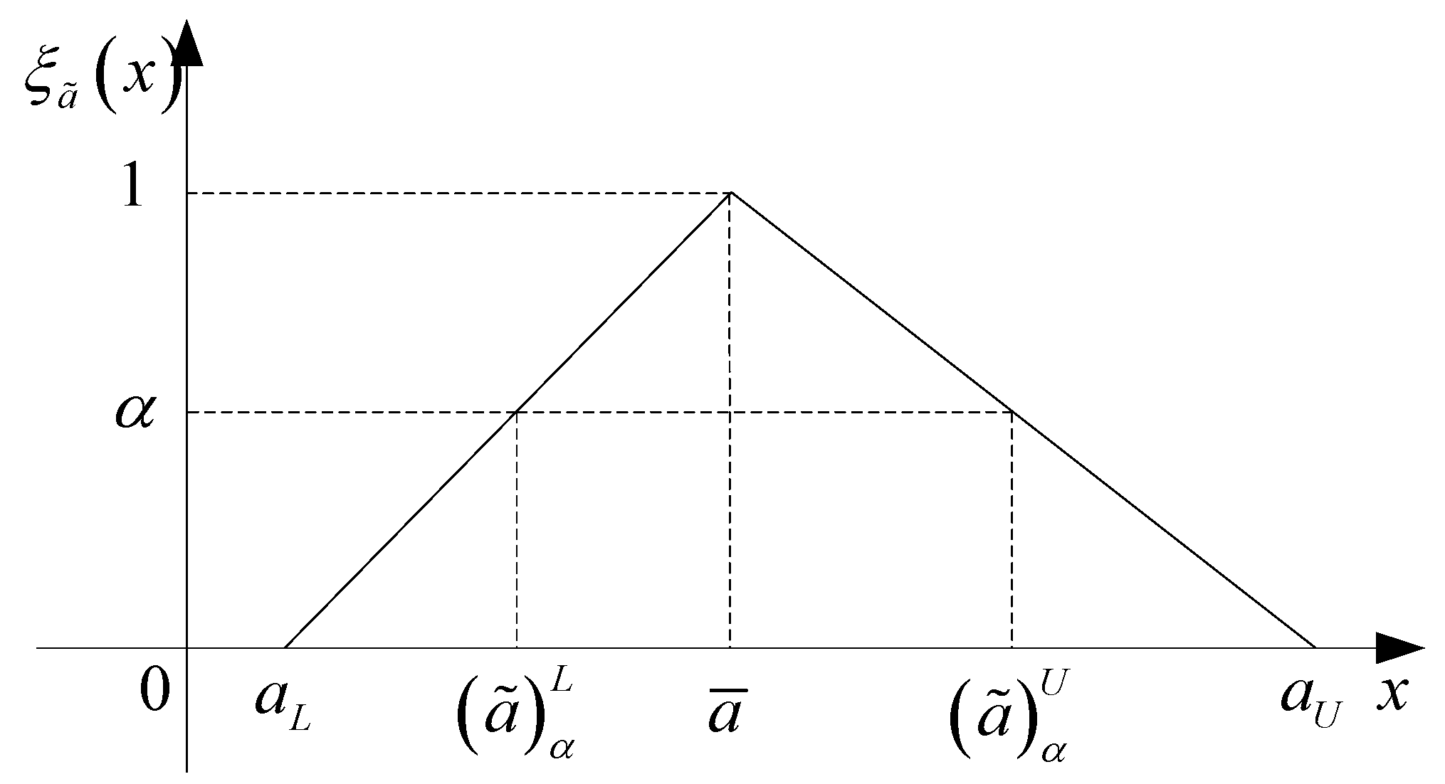
 for all α ∈ [0,1]. In this paper, is also denoted by
  . The α-level set of , shown in Figure 1, is used widely in system reliability analysis.
3. Maximum Entropy Methods


4. Fuzzy Bayesian Reliability Assessment for Deteriorating Components under Small Sample Size Conditions
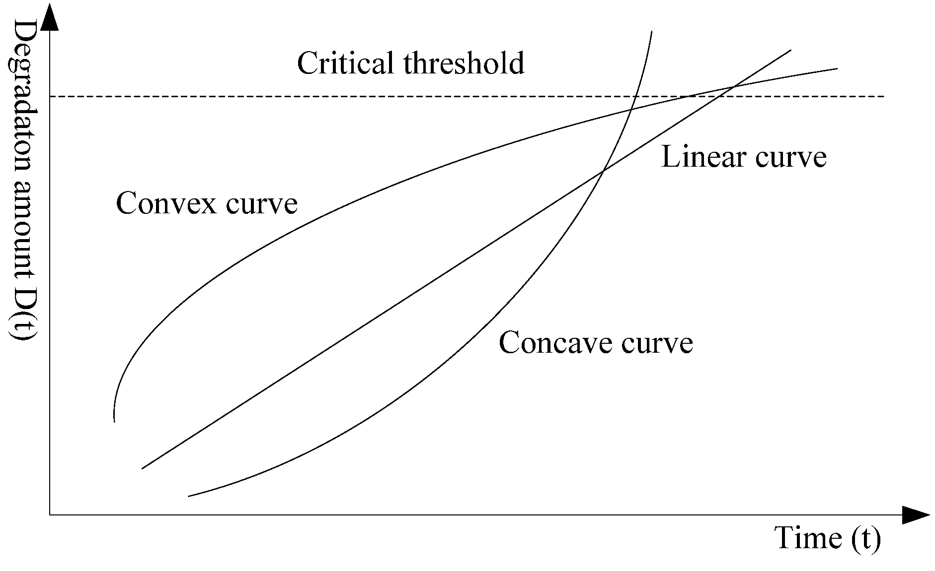
4.1. The Degradation Curve of Deteriorating Components
4.2. Bayesian Reliability Assessment for Deteriorating Components under Small Sample Sizes

| Time t | t0 | t1 | t2 | t3 | … | tj |
|---|---|---|---|---|---|---|
| 1(unit) | D1(t0) | D1(t1) | D1(t2) | D1(t3) | D1(tj) | |
| 2(unit) | D2(t0) | D2(t1) | D2(t2) | D2(t3) | D2(tj) | |
| … | … | … | … | … | … | … |
| n(unit) | Dn(t0) | Dn(t1) | Dn(t2) | Dn(t3) | Dn(tj) |


 is a constant which can be denoted by C(t,λ,π). Therefore, Equation (19) can be rewritten as:


 is a constant.
 .
. , from Equations (1) and (23), the posterior PDF of θ is given by:

 , respectively.


4.3. Fuzzy Bayesian Reliability Assessment for Deteriorating Components


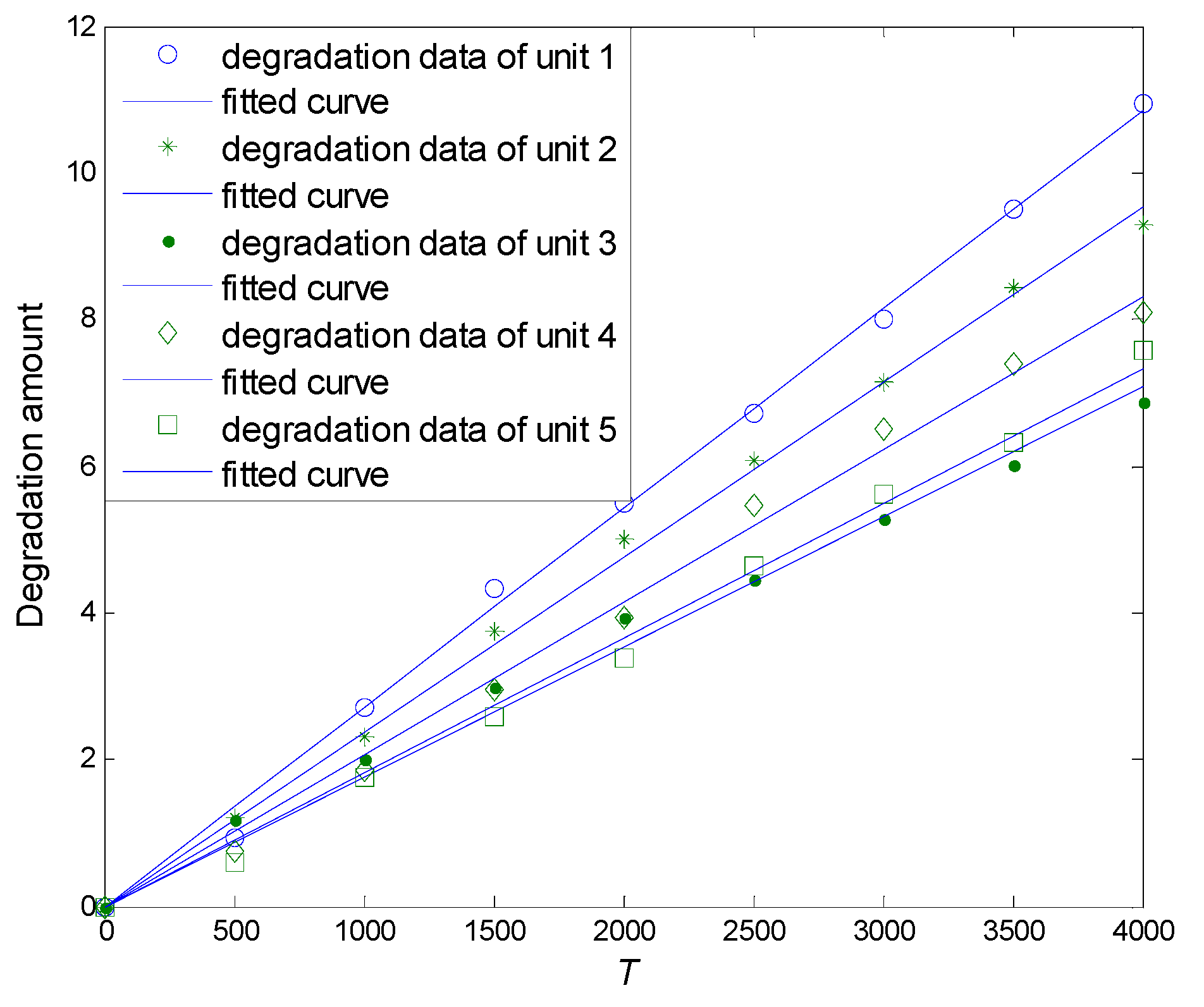
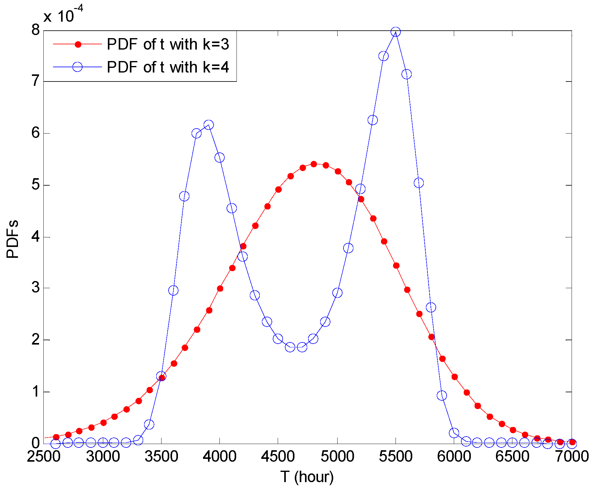
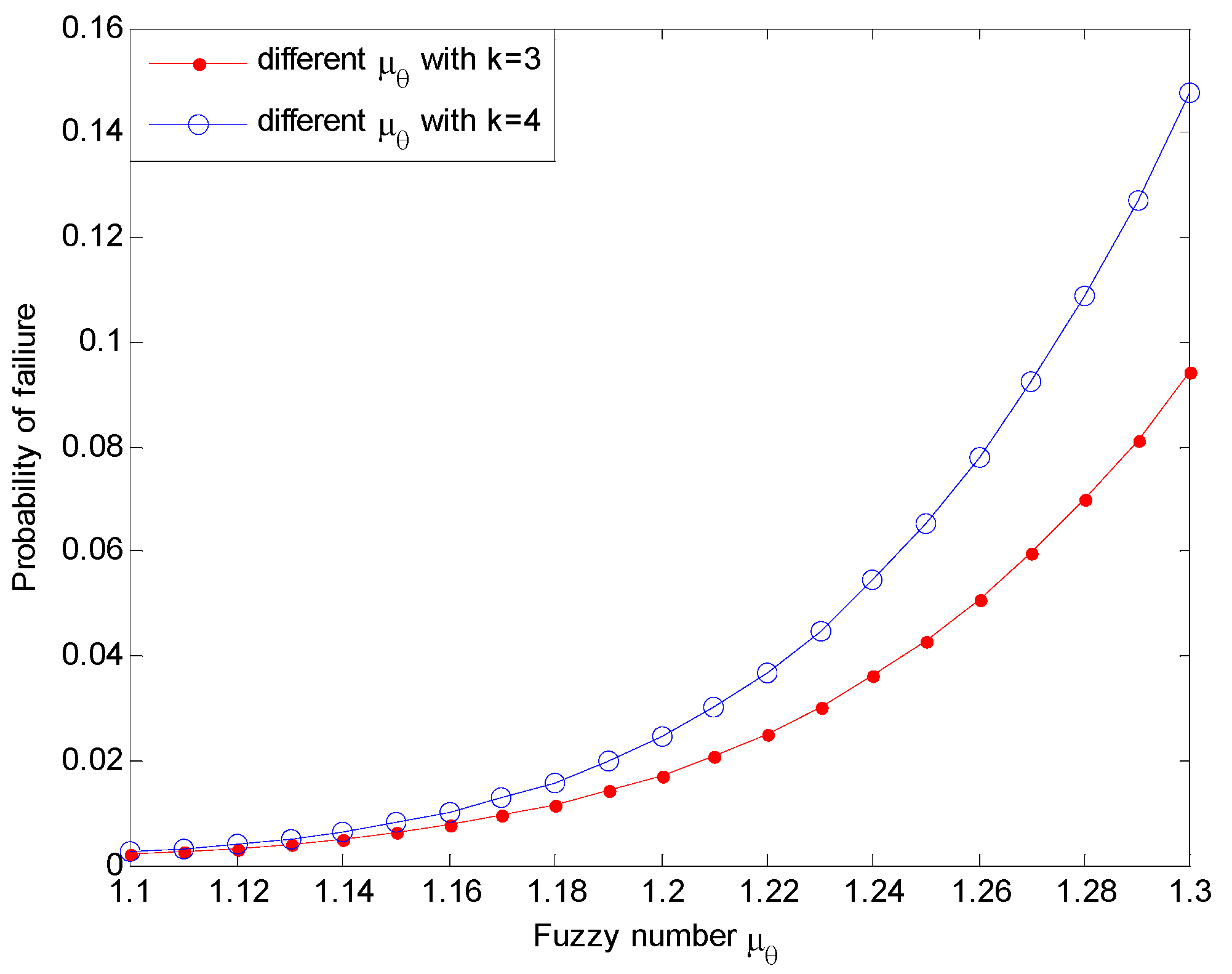
5. Illustrative Examples and Discussion
| t (h) | 0 | 500 | 1000 | 1500 | 2000 | 2500 | 3000 | 3500 | 4000 |
|---|---|---|---|---|---|---|---|---|---|
| 1(unit) | 0 | 0.93 | 2.72 | 4.34 | 5.48 | 6.72 | 8.00 | 9.49 | 10.94 |
| 2(unit) | 0 | 1.22 | 2.30 | 3.75 | 4.99 | 6.07 | 7.16 | 8.42 | 9.28 |
| 3(unit) | 0 | 1.17 | 1.99 | 2.97 | 3.94 | 4.45 | 5.27 | 6.02 | 6.88 |
| 4(unit) | 0 | 0.74 | 1.85 | 2.95 | 3.92 | 5.47 | 6.50 | 7.39 | 8.09 |
| 5(unit) | 0 | 0.61 | 1.77 | 2.58 | 3.38 | 4.63 | 5.62 | 6.32 | 7.59 |


| θ (unit) | 1 | 2 | 3 | 4 | 5 | 6 |
|---|---|---|---|---|---|---|
| value | 1.28 | 1.47 | 1.15 | 1.33 | 1.08 | 1.21 |

| α | 0 | 0.2 | 0.4 | 0.6 | 0.8 | 1.0 |
|---|---|---|---|---|---|---|
| 0.0019 | 0.0030 | 0.0049 | 0.0076 | 0.0116 | 0.0172 | |
| 0.0942 | 0.0698 | 0.0507 | 0.0361 | 0.0252 | 0.0172 |
| α | 0 | 0.2 | 0.4 | 0.6 | 0.8 | 1.0 |
|---|---|---|---|---|---|---|
| 0.0023 | 0.0039 | 0.0063 | 0.0101 | 0.0159 | 0.0245 | |
| 0.1476 | 0.1088 | 0.0779 | 0.0543 | 0.0449 | 0.0245 |

6. Conclusions
Acronyms and Abbreviations
| RV | Random variable |
Probability density function | |
| CDF | Cumulative distribution function |
| MM | Method of moments |
| MLE | Maximum likelihood estimation |
| MEE | Maximum entropy estimation |
| S. | Integral domain |
| λ | Lagrange multipliers |
A fuzzy number | |
Membership function | |
The α-level set of | |
Triangular fuzzy number | |
Prior distribution | |
Maximum entropy density function | |
Posterior PDF | |
| Di(t) | Degradation at time t of unit |
| Df | Critical threshold |
| y. | Given samples |
Acknowledgments
Conflicts of Interest
References
- Nicolai, R.P.; Dekker, R.; van Noortwijk, J.M. A comparison of models for measurable deterioration: An application to coatings on steel structures. Reliab. Eng. Syst. Saf. 2007, 92, 1635–1650. [Google Scholar] [CrossRef]
- Hamada, M.S.; Martz, H.F.; Reese, C.S.; Wilson, A.G. Bayesian Reliability; Springer: New York, NY, USA, 2008. [Google Scholar]
- Pandey, M.D. Probabilistic models for condition assessment of oil and gas pipelines. NDT&E Int. 1998, 31, 349–358. [Google Scholar]
- Tsai, C.C.; Tseng, S.T.; Balakrishnan, N. Optimal burn-in policy for highly reliable products using gamma degradation process. IEEE Trans. Reliab. 2011, 60, 234–245. [Google Scholar] [CrossRef]
- Freitas, M.A.; de Toledo, M.L.G.; Colosimo, E.A.; Pires, M.C. Using degradation data to assess reliability: A case study on train wheel degradation. Qual. Reliab. Eng. Int. 2009, 25, 607–629. [Google Scholar] [CrossRef]
- Pandey, M.D.; van Noortwijk, J.M. Gamma Process Model for Time-Dependent Structural Reliability Analysis. In Proceedings of the Second International Conference on Bridge Maintenance, Safety and Management (IABMAS), Kyoto, Japan, 18–24 October 2004.
- Huang, W.; Dietrich, D.L. An alternative degradation reliability modeling approach using maximum likelihood estimation. IEEE Trans. Reliab. 2005, 54, 310–317. [Google Scholar] [CrossRef]
- Van Noortwijk, J.M.; van der Weide, J.A.M.; Kallen, M.J.; Pandey, M.D. Gamma processes and peaks-over-threshold distributions for time-dependent reliability. Reliab. Eng. Syst. Saf. 2007, 92, 1651–1658. [Google Scholar] [CrossRef]
- Deng, A.M.; Chen, X.; Zhang, C.H.; Wang, Y.-S. Reliability assessment based on performance degradation data. J. Astronaut. 2006, 27, 546–552. (in Chinese). [Google Scholar]
- Savage, G.J.; Son, Y.K. The set-theory method for systems reliability of structure with degrading components. Reliab. Eng. Syst. Saf. 2011, 96, 108–116. [Google Scholar] [CrossRef]
- Stewart, M.G.; Rosowsky, D.V. Time-dependent reliability of deteriorating reinforced concrete bridge decks. Struct. Saf. 1998, 20, 91–109. [Google Scholar] [CrossRef]
- Pandey, M.D.; Yuan, X.X.; van Noortwijk, J.M. The influence of temporal uncertainty of deterioration on life-cycle management of structures. Struct. Infrastruct. Eng. 2009, 5, 145–156. [Google Scholar] [CrossRef]
- Akgül, F.; Frangopol, D.M. Time-dependent interaction between load rating and reliability of deteriorating bridges. Eng. Struct. 2004, 26, 1751–1765. [Google Scholar] [CrossRef]
- Van Noortwijk, J.M.; Klatter, H.E. Optimal inspection decision for the block mats of the eastern-scheldt barrier. Reliab. Eng. Syst. Saf. 1999, 65, 203–211. [Google Scholar] [CrossRef]
- Frangopol, D.M.; Kallen, M.J.; van Noortwijk, J.M. Probabilistic models for life-cycle performance of deteriorating structures: Review and future directions. Prog. Struct. Eng. Mater. 2004, 6, 197–212. [Google Scholar] [CrossRef]
- Abdel-Hameed, M. A gamma wear process. IEEE Trans. Reliab. 1975, 24, 152–153. [Google Scholar] [CrossRef]
- Xiao, N.-C.; Huang, H.-Z.; Wang, Z.-L.; Liu, Y.; Zhang, X.-L. Unified uncertainty analysis by the mean value first order saddlepoint approximation. Struct. Multidiscip. Optim. 2012, 46, 803–812. [Google Scholar] [CrossRef]
- Kiureqhian, A.D.; Ditlevsen, O. Aleatory or epistemic? Does it matter? Struct. Saf. 2009, 31, 105–112. [Google Scholar] [CrossRef]
- Wu, H.C. Bayesian system reliability assessment under fuzzy environments. Reliab. Eng. Syst. Saf. 2004, 83, 277–286. [Google Scholar] [CrossRef]
- Wu, H.C. Fuzzy reliability estimation using Bayesian approach. Comput. Ind. Eng. 2004, 46, 467–493. [Google Scholar] [CrossRef]
- Wu, H.C. The fuzzy estimators of fuzzy parameters based on fuzzy random variables. Eur. J. Oper. Res. 2003, 46, 101–114. [Google Scholar] [CrossRef]
- Taheri, S.M.; Zarei, R. Bayesian system reliability assessment under the vague environment. Appl. Soft Comput. J. 2011, 11, 1614–1622. [Google Scholar] [CrossRef]
- Guida, M.; Penta, F. A Bayesian analysis of fatigue data. Struct. Saf. 2010, 32, 64–76. [Google Scholar] [CrossRef]
- Guikema, S.D. Formulating informative, data-based priors for failure probability estimation in reliability analysis. Reliab. Eng. Syst. Saf. 2007, 92, 490–502. [Google Scholar] [CrossRef]
- Bernardo, J.M.; Smith, A.F.M. Bayesian Theory; Wiley: New York, NY, USA, 2000. [Google Scholar]
- Koch, K.R. Introduction to Bayesian Statistics, 7th ed.; Springer: Berlin, Germany, 2007. [Google Scholar]
- Jaynes, E.T. Information theory and statistical mechanics. Phys. Rev. 1957, 106, 620–630. [Google Scholar] [CrossRef]
- Zelluer, A.; Tobias, J. Further results on Bayesian method of moments analysis of the multiple regression model. Int. Econ. Rev. 2001, 42, 40–121. [Google Scholar]
- Wu, X.M. Calculation of maximum entropy densities with application to income distribution. J. Econ. 2003, 115, 347–354. [Google Scholar] [CrossRef]
- Ormoneit, D.; White, H. An efficient algorithm to compute maximum entropy densities. Econ. Rev. 1999, 18, 127–140. [Google Scholar] [CrossRef]
- Zellner, A.; Highfield, R.A. Calculation of maximum entropy distributions and approximation of marginal posterior distributions. J. Econ. 1988, 37, 195–209. [Google Scholar] [CrossRef]
- Most, T. Efficient structural reliability methods considering incomplete knowledge of random variable distribution. Probabilist. Eng. Mech. 2011, 26, 380–386. [Google Scholar] [CrossRef]
- Cheng, L.; Tong, L. Measurement data processing based on maximum entropy method. J. Electron. Meas. Instrum. 2009, 23, 47–51. (in Chinese). [Google Scholar] [CrossRef]
- Sheng, Z.; Xie, S.Q.; Pan, C.Y. Probability and Mathematical Statistics(in Chinese), 4th ed.; Higher Education Press: Beijing, China, 2008. [Google Scholar]
- Meeker, W.Q.; Escobar, L.A. Statistical Methods for Reliability Data; Wiley: New York, NY, USA, 1998. [Google Scholar]
- Burden, R.L.; Faires, J.D. Numerical Analysis, 7th ed.; Higher Education Press: Bejing, China, 2001. [Google Scholar]
© 2013 by the authors; licensee MDPI, Basel, Switzerland. This article is an open access article distributed under the terms and conditions of the Creative Commons Attribution license (http://creativecommons.org/licenses/by/3.0/).
Share and Cite
Xiao, N.-C.; Li, Y.-F.; Wang, Z.; Peng, W.; Huang, H.-Z. Bayesian Reliability Estimation for Deteriorating Systems with Limited Samples Using the Maximum Entropy Approach. Entropy 2013, 15, 5492-5509. https://doi.org/10.3390/e15125492
Xiao N-C, Li Y-F, Wang Z, Peng W, Huang H-Z. Bayesian Reliability Estimation for Deteriorating Systems with Limited Samples Using the Maximum Entropy Approach. Entropy. 2013; 15(12):5492-5509. https://doi.org/10.3390/e15125492
Chicago/Turabian StyleXiao, Ning-Cong, Yan-Feng Li, Zhonglai Wang, Weiwen Peng, and Hong-Zhong Huang. 2013. "Bayesian Reliability Estimation for Deteriorating Systems with Limited Samples Using the Maximum Entropy Approach" Entropy 15, no. 12: 5492-5509. https://doi.org/10.3390/e15125492