Information-Theoretic Data Discarding for Dynamic Trees on Data Streams

Abstract

Ubiquitous automated data collection at an unprecedented scale is making available streaming, real-time information flows in a wide variety of settings, transforming both science and industry. Learning algorithms deployed in such contexts often rely on single-pass inference, where the data history is never revisited. Learning may also need to be temporally adaptive to remain up-to-date against unforeseen changes in the data generating mechanism. Online Bayesian inference remains challenged by such transient, evolving data streams. Nonparametric modeling techniques can prove particularly ill-suited, as the complexity of the model is allowed to increase with the sample size. In this work, we take steps to overcome these challenges by porting information theoretic heuristics, such as exponential forgetting and active learning, into a fully Bayesian framework. We showcase our methods by augmenting a modern non-parametric modeling framework, dynamic trees, and illustrate its performance on a number of practical examples. The end product is a powerful streaming regression and classification tool, whose performance compares favorably to the state-of-the-art.

1. Introduction

It is a recognized fact that we are now faced with an unprecedented abundance of recorded information in both sciences and industry, a phenomenon often referred to as “Big Data”. An important component of this transformation is the availability of continual real-time information flows in a variety of settings, referred to as data streams. This data deluge is in part the result of recent technological advances, such as cheaper storage, connectivity, computational power and portable “smart” devices, as well as the culmination of a cultural transformation in the commercial world, whereby data are no longer viewed as a stale resource, but rather as a source of actionable insights. Ironically, this massive investment in data collection and management can have an adverse effect on the sophistication of the analyses thereof, as the size of the data can be prohibitive for all but the simplest of methods. This is particularly true of non-parametric Bayesian methods, for technical reasons explained below. And yet, flexible Bayesian methods are in much demand in Big Data, as they can handle diversity without compromising on interpretability.

One way to achieve scalability of learning algorithms is online estimation/inference, where the objective is to develop a set of update equations that incorporate novel information as it becomes available, without needing to revisit the data history. This results in model fitting algorithms whose space and time complexity remains constant as information accumulates, and can hence operate in streaming environments featuring continual data arrival, or navigate massive datasets sequentially. Such operational constraints are becoming imperative in certain application areas as the scale and real-time nature of modern data collection continues to grow.

In certain simple cases, online estimation without information loss is possible via exact recursive update formulae, e.g., via conjugate Bayesian updating (see Section 3.1). In parametric dynamic modeling, approximate samples from the filtering distribution for a variable of interest may be obtained online via sequential Monte Carlo (SMC) techniques, under quite general conditions. SMC is commonly used in non-Gaussian non-linear state-space modeling, where the objective is to sequentially obtain samples from the posterior distribution of the latent state at time t given observations up to that time.

This ability of SMC to draw sequential samples from distributions of increasing dimension renders it an appealing tool for use in Bayesian non-parametric modeling, although this has not yet been widely recognized in the literature. This was pioneered by [1] in the case of dynamic trees, where the tree structure is viewed as the latent state that evolves dynamically. In effect, a “particle cloud” of dynamic trees are employed to track parsimonious regression and classification surfaces as data arrive sequentially. However, the resulting algorithm is not, strictly speaking, online, since tree moves may require access to the full data history, rather than parametric summaries thereof. This complication arises as an essential by-product of non-parametric modeling, wherein the complexity of the estimator is allowed to increase with the dataset size. Therefore, this article recognizes that maintaining constant operational cost as new data arrives necessarily requires discarding some (e.g., historical) data. Trees are a good candidate for such work because both the particle evolution as well as our data discarding ideas are natural and efficient with this particular non-parametric model: several of the operations involved are local to the leaf, and can hence be handled parametrically, as will be seen in detail later.

Specifically, and to help set notation for the remainder of the paper, we consider supervised learning problems with labelled data $({\mathbf{x}}_t,y_t)$, for $t=1,2,\cdots ,T$, where T is either very large or infinite. We consider responses $y_t$ which are real-valued (i.e., regression) or categorical (classification). The p-dimensional predictors ${\mathbf{x}}_t$ may include real-valued features, as well as binary encodings of categorical ones. The dynamic tree model, reviewed shortly in Section 2, allows sequential non-parametric learning via local adaptation when new data arrive. However its complexity, and thus computational time/space demands, may grow with the data size T. The only effective way to limit these demands is to sacrifice degrees-of-freedom (DoF) in representation of the fit, and the simplest way to do that is to discard data; that is, to require the trees to work with a subset $w\ll T$ of the data seen so far.

Our primary concern in this paper is managing the information loss entailed in data discarding. First, we propose datapoint retirement (Section 3), whereby discarded datapoints are partially “remembered” through conjugate informative priors, updated sequentially. This technique is well-suited to trees, which combine non-parametric flexibility with simple parametric models and conjugate priors. Nevertheless, forming new partitions in the tree still requires access to actual datapoints, and consequently data discarding comes at a cost of both information and flexibility. We show that these costs can be managed, to a surprising extent, by employing the right retirement scheme even when discarding data randomly. In Section 4, we further show that active learning heuristics that are designed to maximize the information present in a given subset of the data may be relied upon to prioritize points for retirement. We refer to this technique as active discarding, and show that it leads to better performance still.

An orthogonal concern in streaming data contexts is the need for temporal adaptivity when the concept being learned exhibits drift. This is where the data generating mechanism evolves over time in an unknown way. The bulk of the Bayesian literature has so far focused on dynamic modeling as a means of ensuring temporal adaptivity. However, as explained in Section 5, such models come at great computational expense, typically prohibitive in streaming contexts, and can also be sensitive to model mis-specification. A popular alternative in the streaming data literature is to heuristically modify the given set of recursive update equations to endow it with temporally adaptive properties, commonly via the use of exponential forgetting, whereby the contribution of past datapoints to the algorithm is smoothly downweighed. In Section 5 we demonstrate how this practice can be motivated from an information theoretic perspective. This results in historical data retirement through suitably constructed informative priors that can be easily deployed in the non-parametric dynamic tree modeling context, while remaining fully online. Using synthetic as well as real datasets, we show how this approach compares favorably against modern alternatives. The paper concludes with a discussion in Section 6.

1.1. Relevant Work on Streaming Regression and Classification

Progress in the area of online, temporally adaptive modeling for streaming data has been more forthcoming for classification than regression, presumably because of the fact that streaming data contexts were primarily introduced by the computer science and machine learning communities, which have a cultural preference for discrete responses. In classification, concept drift was introduced as early as 1996 in [2] to denote the fact that temporal variation in data streams that may render past information obsolete and/or misleading. Drift was initially handled via simple modifications to existing algorithms, or sliding window implementations thereof. Incremental trees were discussed in the context of streaming classification by [3,4], who introduced the Very Fast Decision Tree (VFTD) algorithm, and its temporally adaptive counterpart, CVFDT, where leaves that are thought to represent obsolete information are adaptively pruned. Other versions of incrementally updated trees include [5], where learning techniques from neural networks are employed to adaptively update decision trees over streams.

An alternative popular approach has been to maintain a weighted collection of decision trees over the stream, where the weights are adaptively tuned to maintain the best possible “weighted majority vote”. The first instance of the ensemble approach was the Streaming Ensemble Algorithm (SEA) of [6], but several variants have been proposed since, often involving decision trees among their base learners [7,8,9,10]. Yet another approach includes the incorporation of fuzzy rules in the decision tree (e.g., [11]).

Beyond trees, a large variety of adaptive parametric classifiers have been proposed in the literature (see [12] for a review), where often the focus is not on the classifier per se, but rather on successfully managing the trade-off between retaining obsolete information on one hand, and discarding useful historical information on the other. This trade-off is often handled via adaptive forgetting factors, where historical information is smoothly downweighted in an adaptive manner that aims to capture not only the presence, but also the speed of the drift [13]. In [12], it is argued that long-term stability of the data discarding/forgetting mechanism, as opposed to the flexibility of the underlying classifier, can often be the real performance bottleneck in streaming classification, and an approach is proposed that seems to be stable over arbitrarily long time horizons.

Enabling parametric regression models to fare better in streaming domains where the regression surface may be subject to unforeseen temporal variation was pioneered by two communities: the adaptive filtering community in non-stationary statistical signal processing [14]; and the stochastic learning [15] community, which in part evolved from the continuous-response neural networks literature [16]. Both relied on incremental updating equipped with forgetting factors and/or adaptive learning rates, but were exclusively concerned with parametric models. Non-parametric regression modeling has also extensively considered online updating (see [1] for a review), but not temporal drift per se. In part, this is because non-parametric models are flexible enough to accommodate changing regression surfaces by growing in complexity. However, we will later demonstrate that in the event where past information is obsolete and/or misleading, this is an inefficient, or even improper, use of degrees of freedom.

Our work represents a novel contribution in this literature by bringing a variety of key insights about data streams under a coherent Bayesian formalism. First, the particle filter dynamics mimic the behavior of an adaptive ensemble of trees, but enable principled model averaging as opposed to weighted majority votes. Second, the non-parametric tree structure is combined with parametric leaf models, generalizing to a variety of tasks, including both classification and regression. Third, active discarding is considered alongside historical discarding, accommodating more sophisticated data selection than a simple “sliding window”. Third, forgetting factors are incorporated in the leaf priors, enabling us to perform full Bayesian inference in a temporally adaptive fashion. Finally, model complexity is used sensibly, via the combined effect of the tree prior, and up-to-date data selection.

2. Dynamic Trees

Dynamic trees [DT] [1] are a process–analog of Bayesian treed models [17,18]. The model specification is amenable to fast sequential inference by SMC, yielding a predictive surface which organically increases in complexity as more data arrive. Software is available in the dynaTree package [19] for R on CRAN [20], which has been extended to cover the techniques described in this paper. We now review model specification and inference in turn.

2.1. Bayesian Static Treed Models

Trees partition the input space $\mathcal{X}$ into hyper-rectangles, referred to as leaves, using nested logical rules of the form $(x_i\ge c)$. For instance, the partition $(x_1\ge 3)\cap (x_2<-1)$, $(x_1\ge 3)\cap (x_2\ge -1)$ and $(x_1<3)$ represents a tree with two internal nodes and three leaves. We denote by $\eta (\mathbf{x})$ the unique leaf where $\mathbf{x}$ resides, for any $\mathbf{x}\in \mathcal{X}$.

Treed models condition the likelihood function on a tree $\mathcal{T}$ and fit one instance of a given simple parametric model per leaf. In this way, a flexible model is built out of simple parametric models ${({\theta }_{\eta })}_{\eta \in {\mathcal{L}}_{\mathcal{T}}}$, where ${\mathcal{L}}_{\mathcal{T}}$ is the set of leaves in $\mathcal{T}$. This flexibility comes at the price of a hard model search and selection problem: that of selecting a suitable tree structure. In the seminal work of [17], a Bayesian solution to this problem was proposed that relied on a generative prior distribution over trees: a leaf node η may split with probability $p_{\mathrm{split}}(\mathcal{T},\eta )=\alpha {(1+D_{\eta })}^{-\beta }$, where $\alpha ,\beta >0$, and $D_{\eta }$ is the depth of η in the tree $\mathcal{T}$. This induces a joint prior via the probability that internal nodes ${\mathcal{I}}_{\mathcal{T}}$ have split and leaves ${\mathcal{L}}_{\mathcal{T}}$ have not: $\pi (\mathcal{T})\propto {\prod }_{\eta \in {\mathcal{I}}_{\mathcal{T}}}{p}_{\mathrm{split}}(\mathcal{T},\eta ){\prod }_{\eta \in L_{\mathcal{T}}}[1-p_{\mathrm{split}}(\mathcal{T},\eta )].$ The specification is completed by employing independent sampling models at the tree leaves: $p(y_1,\cdots ,y_n|\mathcal{T},{\mathbf{x}}_1,\cdots ,{\mathbf{x}}_n)={\prod }_{\eta \in {\mathcal{L}}_{\mathcal{T}}}p(y^{\eta }|\mathcal{T},{\mathbf{x}}^{\eta })$. Sampling from the posterior proceeds by MCMC, via proposed local changes to $\mathcal{T}$: so-called grow, prune, change, and swap “moves”. Any data type/model may be used as long as the marginal likelihoods $p(y^{\eta }|\mathcal{T},{\mathbf{x}}^{\eta })$ are analytic, i.e., as long as their parameters can be integrated out. This is usually facilitated by fully conjugate, scale invariant, default (non-informative) priors, e.g.,:

$$y\mid \mathbf{x}\sim N\left({\beta }_{\eta (\mathbf{x})}^T\mathbf{x}+{\mu }_{\eta (\mathbf{x})},{\sigma }_{\eta (\mathbf{x})}^2\right),\pi ({\beta }_{\eta (\mathbf{x})},{\mu }_{\eta (\mathbf{x})},{\sigma }_{\eta (\mathbf{x})}^2)\propto \frac{1}{{\sigma }_{\eta (\mathbf{x})}^2}$$

(1)

for linear, or, letting ${\beta }_{\eta }=\mathbf{0}$, constant regression leaves. Similarly, multinomial leaves for classification with Dirichlet priors can be employed. These choices yield analytical posteriors [1] but also efficient recursive updates for incorporating new datapoints (see Section 3.1).

2.2. Dynamic Trees

In DTs the “moves” are embedded into a process, which describes how old trees mature into new ones when new data arrive. Suppose that ${\mathcal{T}}_{t-1}$ represents a set of recursive partitioning rules associated with ${\mathbf{x}}^{t-1}$, the set of covariates observed up-to time $t-1$. The fundamental insight underlying the DT process is to view this tree as a latent state, evolving according to a state transition probability, $P({\mathcal{T}}_t\mid {\mathcal{T}}_{t-1},{\mathbf{x}}_t)$. The dependence on ${\mathbf{x}}_t$ (but not on $y_t$) allows us to consider only moves local to the current observation: i.e., pruning or growing can only occur (if at all) for the leaf $\eta ({\mathbf{x}}_t)$. This builds computational tractability into the process, as we in either case need to recompute in that area. Formally, we let:

$$P({\mathcal{T}}_t\mid {\mathcal{T}}_{t-1},{\mathbf{x}}_t)=\left\{\begin{array}{cc}0,\hfill & \mathrm{if}{\mathcal{T}}_t\mathrm{is\; not\; reachable\; from}{\mathcal{T}}_{t-1}\mathrm{via\; moves\; local\; to}{\mathbf{x}}_t\hfill \\ p_m\pi ({\mathcal{T}}_t),\hfill & \mathrm{otherwise}\hfill \end{array}\right.$$

(2)

where $p_m$ is the probability of the unique move that can produce ${\mathcal{T}}_t$ from ${\mathcal{T}}_{t-1}$, and π is the tree prior. We allow three types of moves: grow, prune and stay moves. Each type is considered equiprobable, whereas for grow moves, we choose among all possible split locations by first choosing a dimension j uniformly at random, and splitting $\eta ({\mathbf{x}}_t)$ around the location $x_j=\xi$ chosen uniformly at random from the interval formed from the projection of $\eta ({\mathbf{x}}_t)$ on the jth input dimension. The new observation, $y_t$, completes a stochastic rule for the update ${\mathcal{T}}_{t-1}\to {\mathcal{T}}_t$ via $p(y^t|{\mathcal{T}}_t,{\mathbf{x}}^t)$ for each ${\mathcal{T}}_t\in \{{\mathcal{T}}_t\}$.

2.3. Sequential Monte Carlo

The DT specification is amenable to Sequential Monte Carlo (SMC), e.g., Particle Learning [21], inferential mechanics. At each iteration t, the discrete approximation to the tree posterior ${\{{\mathcal{T}}_{t-1}^{(i)}\}}_{i=1}^N$, based on N particles, can be updated to ${\{{\mathcal{T}}_t^{(i)}\}}_{i=1}^N$ by resampling and then propagating. Resampling the particles (with replacement) proceeds according to their predictive probability for the next $(\mathbf{x},y)$ pair, $w_i=p(y_t|{\mathcal{T}}_{t-1}^{(i)},{\mathbf{x}}_t)$. Then, propagating each resampled particle follows the process outlined in Section 2.2. Overall, the PL recursion is given by the following formula, where $\mathcal{T}$ encodes both the tree structure, and the leaf parameters:

$$\begin{array}{cc}\hfill p\left({\mathcal{T}}_t\mid {(\mathbf{x},y)}^t\right)& =\int p\left({\mathcal{T}}_t\mid {\mathbf{T}}_{t-1},{\mathbf{x}}_t,y_t\right)dP\left({\mathcal{T}}_{t-1}\mid {(\mathbf{x},y)}^t\right)\hfill \end{array}$$

$$\begin{array}{cc}& \propto \int p\left({\mathcal{T}}_t\mid {\mathbf{T}}_{t-1},{\mathbf{x}}_t,y_t\right)\times p({\mathbf{x}}_t,y_t\mid {\mathcal{T}}_{t-1})dP\left({\mathcal{T}}_{t-1}\mid {(\mathbf{x},y)}^{t-1}\right)\hfill \end{array}$$

Both resampling and propagation are computationally efficient because they involve only local calculations (requiring only the subtrees of the parent of each ${\eta }^{(i)}(\mathbf{x})$). Nevertheless, the particle approximation can shift great distances in posterior space after an update because the data governed by $\eta {({\mathbf{x}}_t)}^{(i)}$ may differ greatly from one particle to another, and thus so may the weights $w_i$. This appealing division of labour mimics the behavior of an ensemble method without explicitly maintaining one. As with all particle simulation methods, some Monte Carlo (MC) error will accumulate and, in practice, one must be careful to assess its effect. Nevertheless, DT out-of-sample performance compares favorably to other nonparametric methods, like Gaussian Process (GP) regression and classification, but at a fraction of the computational cost [1]. A nice byproduct of SMC inference for DTs are reliable marginal likelihoods via the sequential factorization $p(y^T|{\mathbf{x}}^T)\approx \frac{1}{N}{\sum }_{t=1}^{T}logp(y_t|{\mathbf{x}}_t,{\mathcal{T}}_{t-1}^{(i)})$, i.e., using the probabilities calculated in the resample step.

It is worth emphasizing that not all SMC methods for Bayesian trees may serve as the basis of streaming algorithms, since they might be sequential along a dimension other than time. A great example is the recently proposed algorithm of [22]. In the scheme favored in our work, the tth stage of the SMC algorithm results in a distribution over trees, modified (if at all) using the information present in a novel $({\mathbf{x}}_t,y_t)$. In contrast, in [22] the tth stage corresponds to a distribution over trees of depth (at most) t, generated using the entire dataset, which is assumed to have been available offline from the onset.

3. Datapoint Retirement

At time t, the DT algorithm of [1] may need to access arbitrary parts of the data history in order to update the particles. Hence, although sequential inference is fast, the method is not technically online: tree complexity grows as $logt$, and at every update each of the ${\mathbf{x}}^t=\left({\mathbf{x}}_1,\cdots ,{\mathbf{x}}_t\right)$ locations are candidates for new splitting locations via grow. To enable online operation with constant memory requirements, this covariate pool $({\mathbf{x}}^t)$ must be reduced to a size w, constant in t. One way to achieve this is via data discarding. Crucially, the analytic/parametric nature of DT leaves enables a large part of any discarded information to be retained in the form of informative leaf priors. In effect, this yields a soft implementation of data discarding, which we refer to as datapoint retirement. We show that retirement can preserve the posterior predictive properties of the tree even after data are discarded, and furthermore following subsequent prune and stay operations. The only situation where the loss of data hurts is when new data arrive and demand a more complex tree. In that case, any retired points would not be available as anchors for new partitions. Again, since tree operations are local in nature, only the small subtree nearby $\eta ({\mathbf{x}}_t)$ is effected by this loss of DoFs, whereas the complement ${\mathcal{T}}_t\backslash \eta ({\mathbf{x}}_t)$, i.e., most of the tree, is not affected.

3.1. Conjugate Informative Priors at the Leaf Level

Consider first a single leaf $\eta \in {\mathcal{T}}_t$ in which we have already retired some data. That is, suppose we have discarded ${({\mathbf{x}}_s,y_s)}_{\{s\}}$ which was in η in ${\mathcal{T}}_{t^{\prime }}$ at some time $t^{\prime }\le t$. The information in this data can be “remembered” by taking the leaf-specific prior, $\pi ({\theta }_{\eta })$, to be the posterior of ${\theta }_{\eta }$ given (only) the retired data. Suppressing the η subscript, we may take $\pi (\theta )=P\left(\theta \mid {({\mathbf{x}}_s,y_s)}_{\{s\}}\right)\propto L\left(\theta ;{({\mathbf{x}}_s,y_s)}_{\{s\}}\right){\pi }_0(\theta )$ where ${\pi }_0(\theta )$ is a baseline non-informative prior employed at all leaves. The active data in η, i.e., the points which have not been retired, enter into the likelihood in the usual way to form the leaf posterior.

It is fine to define retirement in this way, but more important to argue that such retired information can be updated loslessly, and in a computationally efficient way. Suppose we wish to retire one more datapoint, $({\mathbf{x}}_r,y_r)$. Consider the following recursive updating equation:

$$\begin{array}{cc}\hfill {\pi }^{(\mathrm{new})}(\theta )& =P\left(\theta \mid {({\mathbf{x}}_s,y_s)}_{\{s\},r}\right)\propto L(\theta ;{\mathbf{x}}_r,y_r)P\left(\theta \mid {({\mathbf{x}}_s,y_s)}_{\{s\}}\right)\hfill \end{array}$$

(3)

As shown below, the calculation in Equation (3) is tractable whenever conjugate priors are employed.

Consider first the linear regression model, $\mathbf{y}\sim N(\mathbf{X}\beta ,{\sigma }^2\mathbf{I})$, where $\mathbf{y}={(y_s)}_{\{s\}}$ is the retired response data, and $\mathbf{X}$ the retired augmented design matrix, i.e., whose rows are like ${[1,{\mathbf{x}}_s^{\prime }]}^{\prime }$, so that ${\beta }_1$ represents an intercept. With ${\pi }_0(\beta ,{\sigma }^2)\propto \frac{1}{{\sigma }^2}$, we obtain:

$$\pi (\beta ,{\sigma }^2)=P(\beta ,{\sigma }^2\mid \mathbf{y},\mathbf{X})=\mathrm{NIG}(\nu /2,s\nu /2,\beta ,{\mathcal{G}}^{-1})$$

where NIG stands for Normal-Inverse-Gamma, and assuming the Gram matrix $\mathcal{G}={\mathbf{X}}^{\prime }\mathbf{X}$ is invertible and denoting $Xy={\mathbf{X}}^{\prime }\mathbf{y},r={\mathbf{y}}^{\prime }\mathbf{y}$, we have $\nu =n-p,\beta ={\mathcal{G}}^{-1}Xy$, and $s^2=\frac{1}{\nu }(r-\mathcal{R})$, where $\mathcal{R}=\beta {\mathcal{G}}^{-1}\beta$. Having discarded ${(y_s,{\mathbf{x}}_s)}_{\{s\}}$, we can still afford to keep in memory the values of the above statistics, as, crucially, their dimension does not grow with $|\{s\}|$, and nor does their size, in practice (see Section 3.3 for details on this latter point). Updating the prior to incorporate an additional retiree $(y_r,{\mathbf{x}}_r)$ is easy:

$$\begin{array}{ccccccc}\hfill {\mathcal{G}}^{(\mathrm{new})}& =\mathcal{G}+X_r^{\prime }{X}_r,\hfill & \hfill X{y}^{(\mathrm{new})}& =Xy+{\mathbf{X}}_r^{\prime }{\mathbf{y}}_r,\hfill & \hfill s^{\mathrm{(new)}}& =s+y_r^{\prime }{y}_r,\hfill & \hfill {\nu }^{\mathrm{(new)}}=\nu +1\end{array}$$

(4)

The constant leaf model may be obtained as a special case of the above, where ${\mathbf{x}}^{\star }=1$, $\mathcal{G}=\nu$ and $\beta =\mu$. For the multinomial model, the discarded response values $y_s$ may be represented as indicator vectors ${\mathbf{z}}_s$, where $z_{js}=\mathbf{1}(y_s=j)$. The natural conjugate here is the Dirichlet $D(\mathbf{a})$. The hyperparameter vector $\mathbf{a}$ may be interpreted as counts, and is updated in the obvious manner, namely ${\mathbf{a}}^{(new)}=\mathbf{a}+z_r$ where $z_{jm}=\mathbf{1}(y_r=j)$. A sensible baseline is ${\mathbf{a}}_0=(1,1,\cdots ,1)$. See [23] for more details.

Unfolding the updating Equations (3) and (4) makes it apparent that retirement preserves the posterior distribution. Specifically, the posterior probability of parameters θ, given the active (non-retired) data still in η is

$$\pi (\theta |{\mathbf{x}}^{\eta },y^{\eta })\propto L(\theta ;x^{\eta },y^{\eta })\pi (\theta )\propto L(\theta ;x^{\eta },y^{\eta })L(\theta ;{({\mathbf{x}}_s,y_s)}_{\{s\}}){\pi }_0(\theta )=L(\theta ;x^{{\eta }^{\prime }},y^{{\eta }^{\prime }}){\pi }_0(\theta )$$

where ${\eta }^{\prime }$ is η without having retired ${({\mathbf{x}}_s,y_s)}_{\{s\}}$. Since the posteriors are unchanged, so are the posterior predictive distributions and the marginal likelihoods required for the SMC updates. Note that new data $({\mathbf{x}}_{t+1},y_{t+1})$ which do not update a particular node $\eta \in {\mathcal{T}}_t\to {\mathcal{T}}_{t+1}$ do not change the properties of the posterior local to the region of the input space demarcated by η. It is as if the retired data were never discarded. Only where updates demand modifications of the tree local to η is the loss in active datapoints felt. We argue in Section 3.2 that this impact can be limited to operations which grow the tree locally. Cleverly choosing which points to retire can further mitigate the impact of discarding (see Section 4).

Finally, it is worth mentioning that generalizing our approach to handle non-Gaussian conditional leaves would require non-trivial modifications since neither the posterior nor the MLE would be available in closed-form. We hence defer this to future work.

3.2. Managing Informative Priors at the Tree Level

Intuitively, DTs with retirement manage two types of information: a non-parametric memory comprising an active data pool of constant size $w\ll t$, which forms the leaf likelihoods; and a parametric memory consisting of possibly informative leaf priors. The algorithm we propose proceeds as follows. At time t, add the $t^{\mathrm{th}}$ datapoint to the active pool, and update the model by SMC exactly as explained in Section 2. Then, if t exceeds w, also select some datapoint, $({\mathbf{x}}_r,y_r)$, and discard it from the active pool (see Section 4 for selection criteria), having first updated the associated leaf prior for $\eta {({\mathbf{x}}_r)}^{(i)}$, for each particle $i=1,\cdots ,N$, to “remember” the information present in $({\mathbf{x}}_r,y_r)$. This shifts information from the likelihood part of the posterior to the prior, exactly preserving the time-t posterior predictive distribution and marginal likelihood for every leaf in every tree.

The situation changes when the next data point $({\mathbf{x}}_{t+1},y_{y+1})$ arrives. Recall that the DT update chooses between stay, prune, or grow nearby each $\eta {({\mathbf{x}}_{t+1})}^{(i)}$. Grow and prune moves are affected by the absence of the retired data from the active data pool. In particular, the tree cannot grow if there are no active data candidates to split upon. This informs our assessment of retiree selection criteria in Section 4, as it makes sense not to discard points in parts of the input space where we expect the tree to require further DoFs. Moreover, we recognize that the stochastic choice between the three DT moves depends both upon the likelihood, and retired (prior) information local to $\eta {({\mathbf{x}}_{t+1})}^{(i)}$, so that the way that prior information propagates after a prune, or grow move, matters. The original DT model dictates how likelihood information (i.e., resulting from active data) propagates for each move. We must provide a commensurate propagation for the retired information to ensure that the resulting online trees stay close to their full data counterparts.

If a stay move is chosen stochastically, no further action is required: retiring data has no effect on the posterior. When nodes are grown or pruned, the retiring mechanism itself, which dictates how informative priors can salvage discarded likelihood information, suggests a method for splitting and combining that information. Following a prune, retired information from the pruned leaves, η and its sibling $S(\eta )$, must be pooled into the new leaf prior positioned at the parent $P(\eta )$. Conjugate updating suggests the following additive rule:

$$\begin{array}{cccccccc}\hfill {\mathcal{G}}^{P(\eta )}& ={\mathcal{G}}^{\eta }+{\mathcal{G}}^{S(\eta )},\hfill & \hfill X{y}^{P(\eta )}& =X{y}^{\eta }+X{y}^{S(\eta )}\hfill & \hfill s^{P(\eta )}& =s^{\eta }+s^{S(\eta )},\hfill & \hfill {\nu }^{P(\eta )}& ={\nu }^{\eta }+{\nu }^{S(\eta )}\hfill \end{array}$$

Note that this does not require access to the actual retired datapoints, and would result in the identical posterior even if the data had not been discarded.

A sensible grow move can be derived by reversing this logic. We suggest letting both novel child leaves $\ell (\eta )$ and $r(\eta )$ inherit the parent prior, but split its strength ${\nu }^{\eta }$ between them at proportions equal to the active data proportions in each child. Let $\alpha =\frac{|\ell (\eta )|}{|\eta |}$. Then,

$$\begin{array}{cccccccc}\hfill {\nu }_{\ell (\eta )}& =\alpha {\nu }_{\eta },\hfill & \hfill {\mathcal{G}}^{\ell (\eta )}& =\alpha {\mathcal{G}}^{\eta },\hfill & \hfill X{y}^{\ell (\eta )}& =\alpha X{y}^{\eta },\hfill & \hfill s^{\ell (\eta )}& =\alpha s^{\eta }\hfill \\ \hfill {\nu }_{r(\eta )}& =(1-\alpha ){\nu }_{\eta },\hfill & \hfill {\mathcal{G}}^{r(\eta )}& =(1-\alpha ){\mathcal{G}}^{\eta },\hfill & \hfill X{y}^{r(\eta )}& =(1-\alpha )X{y}^{\eta },\hfill & \hfill s^{r(\eta )}& =(1-\alpha )s^{\eta }\hfill \end{array}$$

In other words, the new child priors share the retired information of the parents with weight proportional to the number of active data points they manage relative to the parent. This preserves the total strength of retired information, preserves the balance between active data and parametric memory, and is reversible: subsequent prune operations will exactly undo the partitioned prior, combining it into the same prior sufficient statistics at the parent.

This brings to light a second cost to discarding data, the first being a loss of candidates for future partitioning. Nodes grown using priors built from retired points lack specific location information from the actual retired $({\mathbf{x}}_s,y_s)$ pairs. Therefore newly grown leaves must necessarily compromise between explaining the new data, e.g., $({\mathbf{x}}_{t+1},y_{t+1})$, with local active data to $\eta {(\mathbf{x})}_{t+1}$, and information from retired points with less localized influence. The weight of each component in the compromise is $|\eta |/(|\eta |+{\nu }_{\eta })$ and ${\nu }_{\eta }/(|\eta |+{\nu }_{\eta })$, respectively. Eventually as t grows, with $w\ll t$ staying constant, retired information naturally dominates, limiting new grows even when active partitioning candidates exist. This means that while the hierarchical way in which retired data filters through to inference (and prediction) at the leaves is sensible, it is doubly-important that data points in parts of the input space where the response is very complex should not be discarded.

Finally, note that although in the original dynamic tree $\mathcal{T}$ referred only to the tree structure and split locations (since all other parameters integrated out), in the presence of retirement, it is used to additionally refer to the informative leaf priors.

3.3. Computational Complexity

The requirement that only $w\ll t$ datapoints are ever kept in memory is necessary but not sufficient to ensure constant memory requirements, as one needs to factor in the size of the model itself—the size of each set of leaf parameters (or equivalently, the respective sufficient statistics), the number of leaves per tree and the total number of trees (particles). We discuss these in turn.

The updates presented in Section 3.1 will, if implemented naïvely, take up space that grows logarithmically with the number of updates (i.e., discarded datapoints $|\{s\}|$), and therefore also with the time index t. Nevertheless, a minor modification can correct this. Consider for instance the following two update equations:

$$X{y}^{(\mathrm{new})}=Xy+{\mathbf{X}}_r^{\prime }{\mathbf{y}}_r,{\mathcal{G}}^{(\mathrm{new})}=\mathcal{G}+X_r^{\prime }{X}_r$$

Although either statistic grows logarithmically with the number of updates, the linear model itself only requires access to ${\mathcal{G}}^{-1}(Xy)$, which in itself does not grow with t. This can be seen by first dividing either statistic by ν to keep their size constant, and then note that

$${\mathcal{G}}^{-1}(Xy)={\left(\mathcal{G}/\nu \right)}^{-1}(Xy/\nu )$$

Note also that the “scaled” versions of $\mathcal{G}$ and $Xy$, given by $\tilde{\mathcal{G}}=\mathcal{G}/\nu$ and $\widetilde{Xy}=Xy/\nu$ can be updated efficiently as follows:

$${\tilde{\mathcal{G}}}^{(\mathrm{new})}=\left(1-\frac{1}{\nu }\right)\tilde{\mathcal{G}}+\frac{1}{\nu }{X}_r^{\prime }{X}_r,{\nu }^{\mathrm{new}}=\nu +1$$

This update also reveals that the updated statistic is a convex combination of the old value of the statistic and the new information, with $\frac{1}{\nu }$ determining the weight of the novel information. Similar convex updates, which we do not list to keep the exposition simple, are possible for all leaf statistics presented so far, except for the “counts” themselves, such as ν. These latter will generally be commensurate to the time index itself t, and hence their space requirements will grow logarithmically with t. However, we argue here that there are good reasons to disregard this in practice.

First, keeping count of the number of datapoints that have been seen so far may be $O(log(t))$, but has an incredibly small leading constant. In particular, in a modern computer, the counter t will take constant space until it exceeds the maximum integer size, which, for a 32 bit computer, is about $4\times {10}^9$, at which point it will require one more byte for another time period of the same length. Consequently, although both $Xy$ and t grow logarithmically with t, the former would be infeasible to maintain naïvely (hence the division by ν) for very large datasets, whereas the latter would require an impossibly large dataset to cause it to exceed a modern computer’s capabilities. The second reason is subtler but perhaps more important. The iteration count is only employed to determine the weight $1/t$ that new information carries in the convex update above. However, $1/(4\times {10}^9)$ is well below a 32 bit computer’s numerical accuracy (more generally, in any given computer, $1/(\max \mathrm{int}\mathrm{size})$ will exceed its numerical accuracy), so that capping t at a very large number and setting $1/t=0$ thereafter would produce a negligible error, impossible to detect in practice. In any case, it is clear that for $\lambda <1$ (which is the recommended setting in streaming contexts anyway, since concept drift is always a possibility), the counter is not an issue since it is bounded above by $\frac{1}{1-\lambda }=O(1)$.

We have demonstrated that, disregarding counts, each leaf takes constant space requirements over time. Moreover, each tree will also have a maximum number of leaves which is a function of the size of the active data pool—this is because of our constraints on the generation on new leaves. Finally, the number of trees is a constant determined in advance. Therefore, overall, our algorithm is computationally capable of handling indefinitely large data streams, which was not the case for [1].

In particular, as a first approximation, the number of leaves is $O(w)$. The most expensive operation per leaf per timestep (per particle) is the inversion of the Gram matrix in the linear regression case which requires $O(p^3)$ computations (faster Sherman-Morrison-type [24] sequential updates for the inverse Gram are not possible for grow moves). At any given time, only updates local to the datapoint in question will take place, so the total computation spent per particle will comprise a search over all leaves, followed by a local update, i.e., $O(wp+p^3)$. Active discarding adds a $O(p^2{\sum }_{i=1}^N|{\eta }^{(i)}(x)|)$ term (see Section 4.4), which can be bounded above by $O(w{p}^2)$. Since $w\gg p$, we may simplify the total computation per timestep as $O(N{p}^3)$.

3.4. Discussion: Effect of Retirement on SMC Properties

Formally, retiring datapoints changes the posterior distribution, so that the SMC algorithm is tracking a moving target. Obtaining theoretical guarantees in such a setting lies beyond the scope of this paper. Nevertheless, the following thought experiment suggests that our proposal is a valid candidate for an approximate SMC algorithm.

For sufficiently large data, it is not unreasonable to assume that the full data posterior distribution will become increasingly peaked. This also applies to its non-parametric component. Put differently, as the sample size grows, we might assume that the posterior distribution will eventually place most of its mass on a finite number of fixed tree structures, each of finite complexity. At that point, it would be possible to retire all but a fixed number of datapoints without any change to the predictive posterior distribution. In principle, therefore, it seems possible for some fixed memory SMC with a sufficiently large but finite active data pool, to approximate the full data SMC arbitrarily well. The question then becomes one of coming up with the best selection mechanism that discards datapoints in such a manner so as to minimize disruption during the learning process, as well as minimize the mismatch between the “optimal” set of tree structures and the set of tree structures that is “reachable” via the active pool.

We conjecture that random discarding with a forgetting factor $\lambda \approx 1$ but not equal to 1 is the safest option, in that, assuming data exchangeability, the SMC is given ample opportunity to correct any mistakes by virtue of the lower bound on the entropy of the leaf posteriors which is enforced by the forgetting factor (it precludes peaking). For $\lambda =1$, in contrast, it is possible for any given particle to be misled during initial learning and never recover, although resampling over a large enough particle cloud will certainly moderate the impact of such “local optima”.

Active discarding, which is discussed in the next section, is a higher-risk higher-reward alternative that has the potential to offer great improvements over random discarding, but can also introduce subtle and potentially hard to control forms of bias—in particular since the order in which datapoints are seen and potentially removed matters. Motivating such selection mechanisms purely from theoretical arguments would require a formal understanding of the non-parametric information present in a datapoint within the context of an SMC algorithm, which seems intractable at the moment. Given the pressing need to come up with scalable, online inference for flexible models, it seems to us that quicker progress may be made via empirical evaluation of sensible, informed heuristics, inspired from active learning theory, which may in turn drive future theoretical development.

4. Active Discarding

It matters which data points are chosen for retirement, so it is desirable to retire datapoints that will be of “less” use to the model going forward. In the case of a drifting concepts, retiring historically, i.e., retiring the oldest datapoints, may be sensible. We address this in Section 5. Here we consider static concepts, or in other words i.i.d. data. We formulate the choice of which active data points to retire as an active discarding (AD) problem by borrowing (and reversing) techniques from the active learning (AL) literature—this analogy is described in Section 4.1. Regression and classification models are handled separately, as they require different AD techniques, in Section 4.2 and Section 4.3 respectively. We shall see that in both cases AD is, in fact, computationally easier than AL since DTs enable thrifty analytic calculations not previously possible, which are easily updated within the SMC.

4.1. Active Learning versus Active Discarding

Retiring a point $({\mathbf{x}}_r,y_r)$ hurts the SMC algorithm in various ways, among which the most important is that it can make locations near ${\mathbf{x}}_r$ unavailable as potential future splits, and consequently some leaves might become depopulated. Therefore, the decision of which datapoint to retire might be seen as analogous to that of which locations the model would like to continue learning about. In this sense, we seem to be facing the inverse of an active learning problem: which area of the input space is most likely to produce informative observations? As in active learning, there are more than one ways to specify what we mean by “informative”. We draw on the active learning literature to make that notion more precise in Section 4.2 and Section 4.3, for classification and regression respectively.

Although it allows us to make quick progress in coming up with sensible candidate heuristics to be evaluated empirically, the analogy with active learning is not complete enough to act as a theoretical justification. Indeed, the information-theoretic motivation of active learning heuristics is not readily applicable to any non-parametric setting, let alone the much more intricate problem of active discarding within SMC, which, to our knowledge, we are the first to consider. Despite their elusive formal justification, active learning heuristics remain both popular and successful in non-parametric settings, and, in similar fashion, they seem to be sufficiently relevant in our case to yield statistically significant benefits over random discarding in our experiments. Such evidence is valuable in carving out a research direction in this novel research problem. In contrast, the alternative of formally pinning down the exact nature of the information loss entailed by data retirement and managing it in a provably optimal manner seems theoretically intractable at the moment.

4.2. Active Discarding for Regression

Active learning (AL) procedures are sequential decision heuristics for choosing data to add to the design, usually with the aim of minimizing prediction error. Two common AL heuristics are active learning MacKay ([25], ALM) and active learning Cohn ([26], ALC). They were popularized in the modern nonparametric regression literature [27] using GPs, and subsequently ported to DTs [1]. An ALM scheme selects new inputs ${\mathbf{x}}^{\star }$ with maximum variance for $y({\mathbf{x}}^{\star })$, whereas ALC chooses ${\mathbf{x}}^{\star }$ to maximize the expected reduction in predictive variance averaged over the input space. Both approximate maximum expected information designs in certain cases. ALC is computationally more demanding than ALM, requiring an integral over a set of reference locations that can be expensive to approximate numerically for most models. But it leads to better exploration when used with nonstationary models like DTs because it concentrates sampled points near to where the response surface is changing most rapidly [1]. ALM has the disadvantage that it does not cope well with heteroskedastic data (i.e., input-dependent noise). It can end up favoring regions of high noise rather than high model uncertainty. Both are sensitive to the choice of (and density of) a search grid over which the variance statistics are evaluated.

Our first simplification when porting AL to AD is to recognize that no grids are needed. We focus on the ALC statistic here because it is generally preferred, but also to illustrate how the integrals required are actually very tractable with DTs, which is not true in general. The AD program is to evaluate the ALC statistic at each active data location, and choose the smallest one for discarding. AL, by contrast, prefers large ALC statistics to augment the design. We focus on the linear leaf model, as the constant model may be derived as a special case. For an active data location $\mathbf{x}$ and (any) reference location $\mathbf{z}$, the reduction in variance at $\mathbf{z}$ given that $\mathbf{x}$ is in the design, and a tree $\mathcal{T}$ is given by (see [1]):

$$\Delta {\sigma }_{\mathbf{x}}^2(\mathbf{z}|\mathcal{T})=\Delta {\sigma }_{\mathbf{x}}^2(\mathbf{z}|\eta )\equiv {\sigma }^2(\mathbf{z}|\eta )-{\sigma }_x^2(\mathbf{z}|\eta )=\frac{s_{\eta }^2-{\mathcal{R}}_{\eta }}{|\eta |-m-3}\times \frac{{\left(\frac{1}{|\eta |}+{\mathbf{z}}^{\prime }{\mathcal{G}}_{\eta }^{-1}\mathbf{x}\right)}^2}{1+\frac{1}{|\eta |}+{\mathbf{x}}^{\prime }{\mathcal{G}}_{\eta }^{-1}\mathbf{x}}$$

when both $\mathbf{x}$ and $\mathbf{z}$ are in $\eta \in {\mathcal{L}}_{\mathcal{T}}$, and zero otherwise, and the expression for ${\sigma }_x^2(\mathbf{z}\mid \eta )$ is given by the standard formulae for Bayesian parametric linear regression, e.g., ([28], Chapter 14). This expression is valid whether learning or discarding, however AL requires evaluating $\Delta {\sigma }^2(x)$ over a dense candidate grid of x’s. AD need only consider the current active data locations, which can represent a dramatic savings in computational cost.

Integrating over $\mathbf{z}$ gives:

$$\Delta {\sigma }^2(\mathbf{x})={\int }_{{\mathbb{R}}^d}\Delta {\sigma }_{\mathbf{x}}^2(\mathbf{z})d\mathbf{z}=\frac{s_{\eta }^2-{\mathcal{R}}_{\eta }}{(|\eta |-m-3)(1+\frac{1}{|\eta |}+{\mathbf{x}}^{\prime }{\mathcal{G}}_{\eta }^{-1}\mathbf{x})}\times {\int }_{\eta }{\left(\frac{1}{|\eta |}+{\mathbf{z}}^{\prime }{\mathcal{G}}_{\eta }^{-1}\mathbf{x}\right)}^{2}d\mathbf{z}$$

The integral that remains, over the rectangular region η, is tedious to write out but has a trivial $O(p^2)$ implementation. Let the p-rectangle η be described by ${\{(a_i,b_i)\}}^p$. Then,

$$\begin{array}{cc}\hfill {\int }_{a_1}^{b_1}& \cdots {\int }_{a_p}^{b_p}{\left(c+\sum _{i=1}^p{\tilde{z}}_i{x}_i\right)}^{2}d{z}_1\cdots d{z}_p=A_{\eta }{c}^2+c\sum _i\left(\prod _{k\ne i}(b_k-a_k)\right)x_i(b_i^2-a_i^2)\hfill \\ & +\sum _i\left(\prod _{k\ne i}(b_k-a_k)\right)\frac{x_i^2}{3}(b_i^3-a_i^3)+\sum _i\sum _{j<i}\left(\prod _{k\ne i,j}(b_k-a_k)\right)\frac{x_i{x}_j}{2}(b_i^2-a_i^2)(b_j^2-a_j^2)\hfill \end{array}$$

where $\tilde{\mathbf{z}}={\mathbf{z}}^{\prime }{\mathcal{G}}_{\eta }^{-1}$, and $c=1/|\eta |$. A general-purpose numerical version via sums using R reference locations $\mathbf{z}$—previously the state of the art [1]—requires $O(Rp)$ computation with R growing exponentially in p for reasonable accuracy (e.g., a hypercube on p dimensions requires $2^p$ points). Observe that the rectangular leaf regions generated by the trees is key. In the case of other partition models (like Voronoi tessellation models), this analytical integration would not be possible.

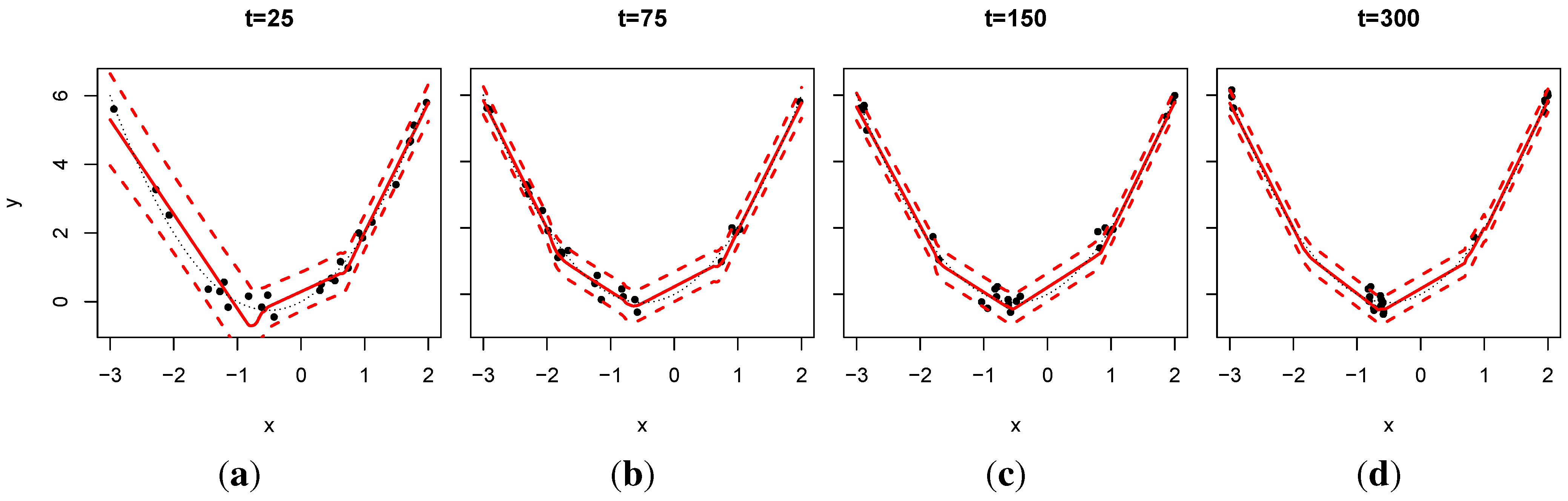
In Figure 1, we observe that in repeated applications of ALC for AD the active points that remain tend shuffle themselves so that they cluster near the high posterior partitioning boundaries, which makes sense because these are the locations where the predictive surface is changing the fastest. The number of such locations depends on the number of active data points allowed, w.

Figure 1. Snapshots of active data (25 points) and predictive surfaces spanning 275 retirement/updating rounds; $Y(x)=x+x^2+\epsilon$, $\epsilon \sim \mathcal{N}(0,1)$.

Figure 1. Snapshots of active data (25 points) and predictive surfaces spanning 275 retirement/updating rounds; $Y(x)=x+x^2+\epsilon$, $\epsilon \sim \mathcal{N}(0,1)$.

As an illustration, consider the simple example where the response is a parabolic function, which must be learned sequentially via x-data sampled uniformly in $(-3,2)$, with $w=25$. The initial 25, before any retiring, are shown in the first panel. Each updating round then proceeds with one retirement followed by one new pair, and subsequent SMC update. Since the implementation requires at least five points in each leaf, seeing four regimes emerge is perhaps not surprising. By $t=150$, the third pane, the ability to learn about the mean with just 25 degrees of freedom is saturated, but it is possible to improve on the variance (shown as errorbars), which are indeed smaller in the final $t=300$ pane. Eventually, the points will cluster at the ends because that is where the response is changing most rapidly, and indeed the derivative is highest there (in absolute value).

4.3. Active Discarding for Classification

For classification, predictive entropy is an obvious AL heuristic. Given a predictive surface comprised of probabilities $p_{\ell }(\mathbf{x})$ for each class ℓ, from DTs or otherwise, the predictive entropy at $\mathbf{x}$ is $-{\sum }_{\ell }{p}_{\ell }(\mathbf{x})log{p}_{\ell }(\mathbf{x})$. Entropy can be an optimal method for measuring predictive uncertainty, but that does not mean it is good for AL. Many authors (e.g., [29]) have observed that it can be too greedy: entropy can be very high near the best explored class boundaries. Several, largely unsatisfactory, remedies have been suggested in the literature. Fortunately, no remedy is required for the AD analog, which focuses on the lowest entropy active data, a finite set. The discarded points will tend to be far into the class interior, where they can be safely subsumed into the prior. Their spacing and shifting of the active pool is quite similar to discarding by ALC for regression, and so we do not illustrate it here.

4.4. Fast Local Updates of Active Discarding Statistics with Trees

The divide and conquer nature of trees—whose posterior distribution is approximated by thrifty, local, particle updates—allows AD statistics to be updated cheaply too. If each leaf node stores its own AD statistics, it suffices to update only the ones in leaf nodes which have been modified, as described below. Any recalculated statistics can then be subsumed into a global, particle averaged, version. Note that no updates to the AD statistics are needed when a point is retired since the predictive distributions are unchanged.

When a new datapoint $(\mathbf{x},y)$ arrives, the posterior undergoes two types of changes: resample then propagate. In the resample step the discrete particle distribution changes, although the trees therein do not change. Therefore, each discarded particle must have its AD statistics (stored at the leaves) subtracted from the full particle tally. Then each correspondingly duplicated particle can have its AD statistics added in. No new integrals (for ALC) or entropy calculations (for classification) are needed. In the propagate step, each particle undergoes a change local to $\eta {(\mathbf{x})}^{(i)}\in {\mathcal{T}}_t^{(i)}$. This requires first calculating the AD statistic for the new $(\mathbf{x},y)$ for each ${\eta }^{(i)}(\mathbf{x})$, before the dynamic update occurs, and then swapping it into the particle average. New integrations, etc., need evaluating here. Then, each non-stay dynamic update triggers swap of the old AD statistics in ${\eta }^{(i)}(\mathbf{x})$ for freshly re-calculated ones from the leaf node(s) in ${\mathcal{T}}_{t+1}^{(i)}$. The total computational cost is in $O(p^{2}N)$ for incorporating $(\mathbf{x},y)$ into N particles, plus $O(p^2{\sum }_{i=1}^N|{\eta }^{(i)}(x)|)$ to update the leaves. One might imagine a thriftier, but harder to implement version, which waits until the end to calculate the AD statistic for the new point $(x,y)$. But it would have the same computational order.

4.5. Empirical Results

Here we explore the benefit of AD over simpler heuristics, like random discarding and subsetted data estimators, by making predictive comparisons on benchmark regression and classification data. All results use the publicly available R implementation of dynaTree available in CRAN, in a fashion analogous to the demonstrator routines demo("online") and demo("elec2")

To focus the discussion on our key objective for this section, we employ moderate data sample sizes in order to allow a comparison to full-data versions of DTs, and assess the impact of data discarding on performance. In particular, we do not repeat here a comparison of full-data DTs to competitors, which may be found in [1], but emphasize that discarding enables DTs to operate on (arbitrarily long) data streams, where the original DTs, as well as their main GP-based competitors, will eventually become intractable. This is better illustrated by the use of massive and streaming classification datasets in Section 5.

4.5.1. Simple Synthetic Regression Data

We first consider data originally used to illustrate multivariate adaptive regression splines (MARS) [30], and then to demonstrate the competitiveness of DTs relative to modern (batch) nonparametric models [1]. The response is $10sin(\pi x_1{x}_2)+20{(x_3-0.5)}^2+10x_4+5x_5$ plus $\mathcal{N}(0,1)$ additive error. Inputs $\mathbf{x}$ are random in ${[0,1]}^5$. To allow a direct comparison with [1] we run a shorter experiment with a total sample size of $2,000$, but also include a longer experiment with sample size $20,000$. We considered four estimators: one based on 100 pairs (ORIG), one based on making use of the entire dataset (FULL), and two online versions using either random (ORAND) or ALC (OALC) retiring to keep the total active data set limited to $w=100$. ORIG is intended as a lower benchmark, representing a naïve fixed-budget method; FULL is at the upper end.

The full experiment comprised 100 repeats in a MC fashion, each with new random training sets, and random testing sets of size 1,000. $N=1,000$ particles and a linear leaf model were used throughout. Similar results were obtained for the constant model.

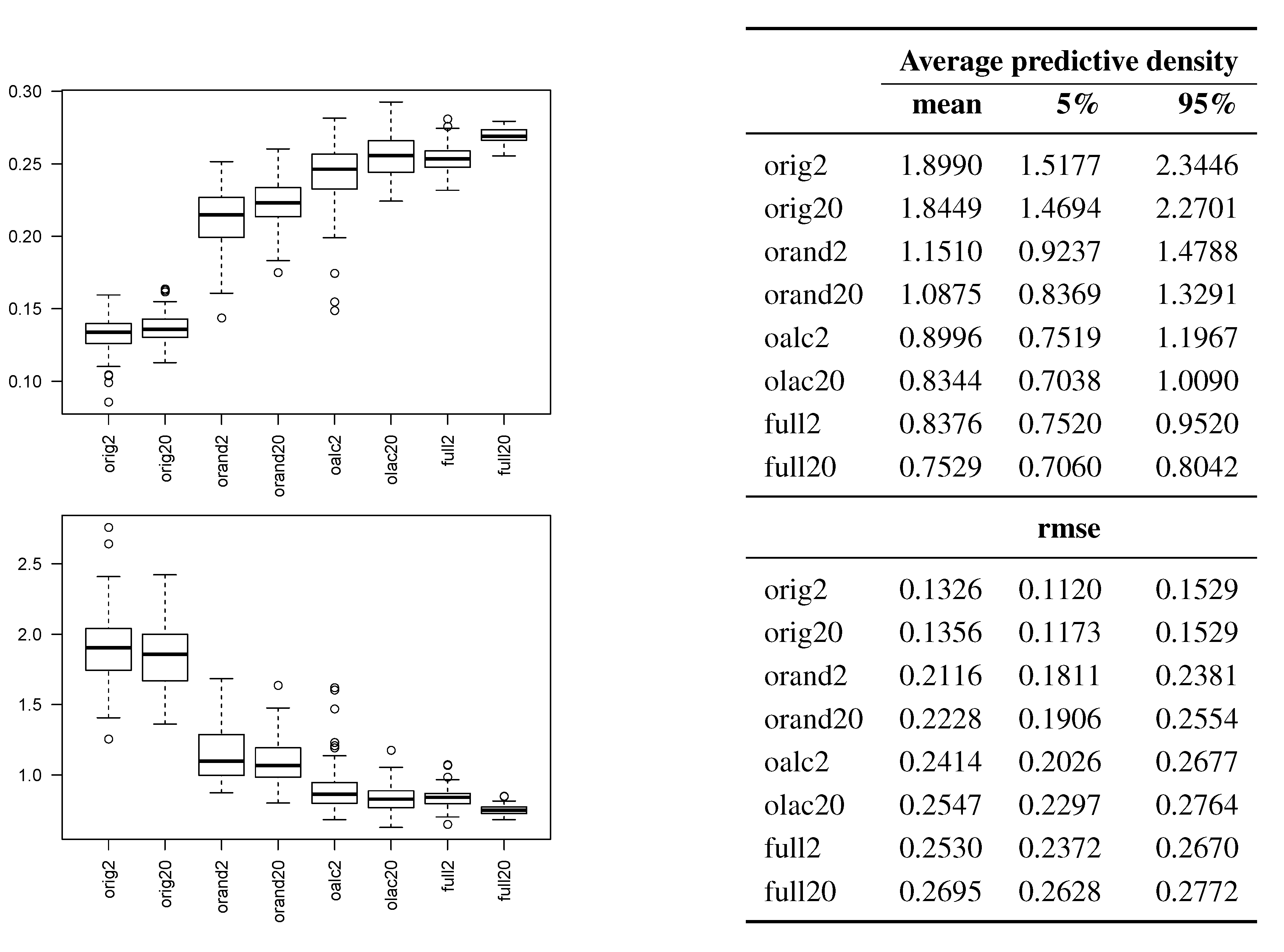
Figure 2 reveals that random retiring is better than subsetting, but retiring by ALC is even better, and can be nearly as good as the full-data estimator. This conclusion persists across both the smaller and larger experiment, with only moderate performance improvements in the latter case. In fact, OALC was the best predictor 16% and 28% of the time by average predictive density and RMSE, respectively. The average time used by each estimator was approximately 1, 33, 45, and 67 seconds, respectively. So random retiring on this modestly-sized problem is 2-times faster than using the full data. ALC costs about 18% extra, time-wise, but leads to about a 35% reduction in RMSE relative to the full estimator. The time-demands of the full estimator grow roughly as $tlogt$, whereas the online versions stay constant. This required a significant amount of computation for the 20,000 dataset, needing almost 4 GB of RAM, whereas the online versions’ requirements were in the order of megabytes instead.

Figure 2. Friedman data comparisons by average posterior predictive density (higher is better) and RMSE (lower is better). A suffix of “20”, as opposed to “2”, indicates the larger experiment with a sample size of 20,000.

Figure 2. Friedman data comparisons by average posterior predictive density (higher is better) and RMSE (lower is better). A suffix of “20”, as opposed to “2”, indicates the larger experiment with a sample size of 20,000.

It was also interesting to observe the tree characteristics across different methods. In the larger experiment, OALC grew to an average depth of about 6 (12 leaves, with 8 active and 150 retired points each), whereas FULL achieved depths of about 25, with about 20 points in each. These results emphasize the fact that the bound on the active data pool in the online algorithms poses a constraint not only on available information, but also on the maximum depth of the trees. Under such constraints, the small difference in performance between FULL and OALC seems promising.

4.5.2. Spam Classification Data

Now consider the Spambase data set, from the UCI Machine Learning Repository [31]. The data contains binary classifications of 4601 emails based on 57 attributes (predictors). We report on a similar experiment to the Friedman/regression example, above, except with classification leaves and 5-fold CV to create training and testing sets. This was repeated twenty times, randomly, giving 100 sets total. Again, four estimators were used: one based on 1/10 of the training fold (ORIG), one based on the full fold (FULL), and two online versions trained on the same stream(s) using either random (ORAND) or entropy (OENT) retiring to keep the total active data set limited to 1/10 of the full set.

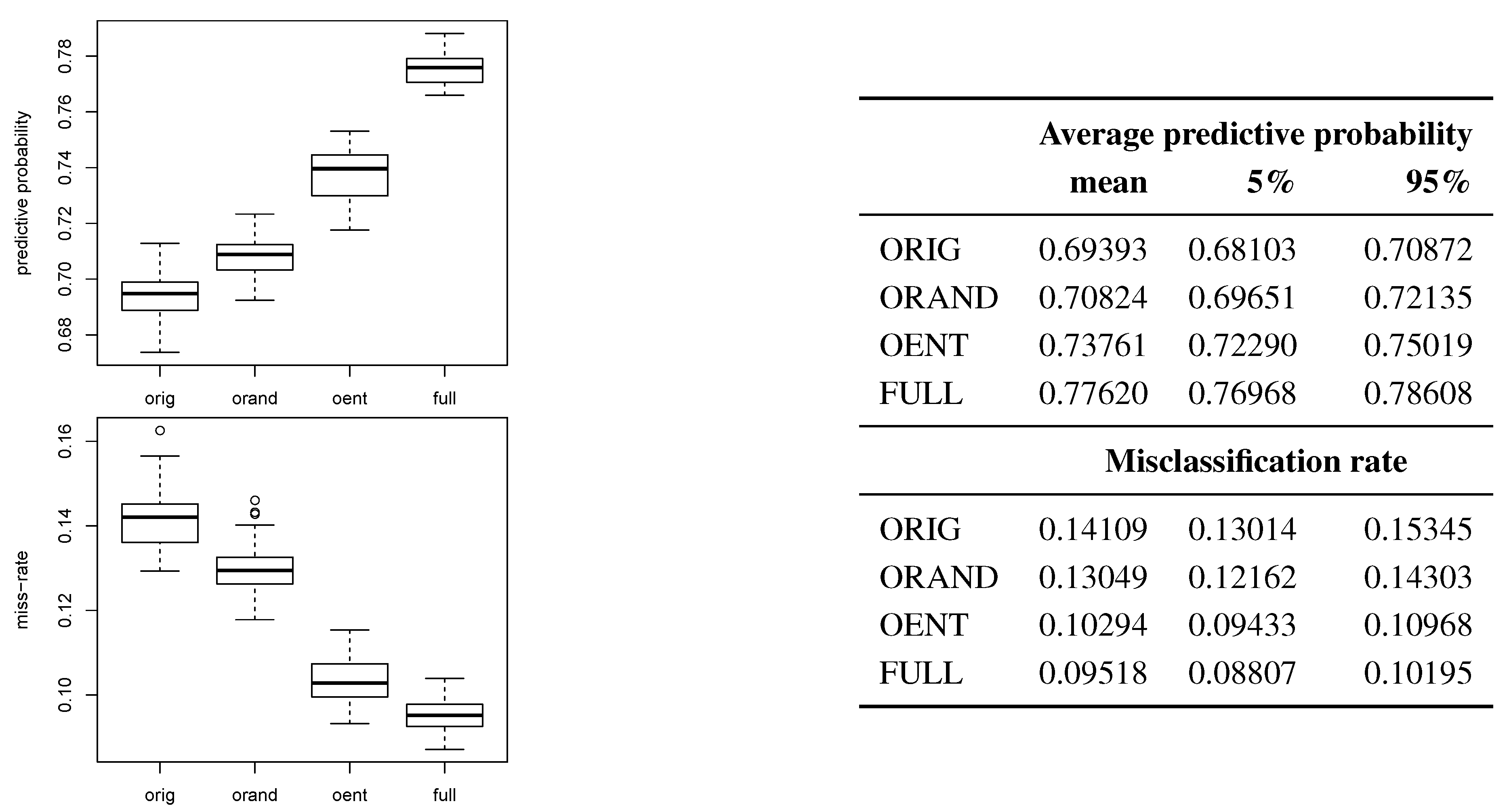
Figure 3 tells a similar story to the Friedman experiment: random discarding is better than subsetting, but discarding by entropy is even better, and can be nearly as good as the full-data estimator. Entropy retiring resulted the best predictor 7% of the time by misclassification rate, but never by posterior predictive probability.

Figure 3. Spam data comparisons by average posterior predictive probability (higher is better) and misclassification rate (lower is better) on the testing set(s).

Figure 3. Spam data comparisons by average posterior predictive probability (higher is better) and misclassification rate (lower is better) on the testing set(s).

To give some indication of comparative performance, we run a single experiment of our proposed method against several state-of-the-art online classifiers, implemented in [32]. In addition to SPAM, we included a larger dataset, ELEC2 (comprising more than 25K observations), described in [33] and commonly used in studies of streaming classification performance. However, as none of the classifiers in [32] is designed to handle concept drift, we additionally randomly shuffled ELEC2 to remove any time-dependence. The results are shown in Table 1. It is clear that the performance of the proposed method is competitive with the state-of-the-art, with OENT featuring in both cases among the top 3 performers.

Table 1. Misclassification rate (lower is better) of variants of dynamic trees against four state-of-the-art streaming classifiers described in [32].

	FULL	OENT	ORAND	MCLP Boost	Random Forest	MC Boost	LaRank
SPAM	0.205	0.126	0.163	0.06	0.125	0.08	0.332
ELEC2	0.271	0.270	0.268	0.459	0.335	0.309	0.401

Table 1. Misclassification rate (lower is better) of variants of dynamic trees against four state-of-the-art streaming classifiers described in [32].

	FULL	OENT	ORAND	MCLP Boost	Random Forest	MC Boost	LaRank
SPAM	0.205	0.126	0.163	0.06	0.125	0.08	0.332
ELEC2	0.271	0.270	0.268	0.459	0.335	0.309	0.401

5. Handling Drift Using Forgetting Factors

The accumulation of historical information at the leaf priors introduced by data retirement may eventually overpower the likelihood of active datapoints. This is natural in an i.i.d. setting, but may cause performance deterioration in streaming contexts where the data generating mechanism may evolve or change suddenly. To promote responsiveness, we may exponentially downweight the retired data history s when retiring an additional point $y_m$. The term power priors was coined in [34] to refer to the resulting modified Bayesian update formula:

$$P^{(\lambda )}(\theta \mid D,D_0)\propto L(\theta ;D)L^{\lambda }(\theta ;D_0){\pi }_0(\theta )$$

In effect, the power prior is a family of priors for $\lambda \in [0,1]$, where $\lambda =0$ is tantamount to ignoring the data $D_0$ and falling back to the data-independent initial prior, whereas $\lambda =1$ is identical to an ordinary Bayesian update, whereby no distinction is made between novel and historical data. The authors in [34] proceed to prove that for $\lambda \in (0,1)$, we have:

$$P^{(\lambda )}(\theta \mid D,D_0)=\underset{g}{\mathrm{argmin}}\left\{\lambda \mathrm{KL}(g,P(\theta \mid D))+(1-\lambda )\mathrm{KL}(g,P(\theta \mid D,D_0))\right\}$$

This suggests that $P^{(\lambda )}(\theta \mid D,D_0)$ is an “interpolation” (in the KL-divergence sense) between $P(\theta \mid D)$ and $P(\theta \mid D,D_0)$, a desirable and intuitive property. In [35], it is also shown that $P^{(\lambda )}(\theta \mid D)$ may be understood as the maximum entropy distribution that lies within a certain distance α (in the KL-sense) from $P(\theta \mid D,D_0)$, where α is the Lagrangian version of the constant λ. This emphasizes the dual property of power priors: in addition to downweighing historical information, they increase the distribution’s uncertainty to reflect the fact that data has been discarded. This results in posterior distributions that are more nuanced, and centered around more recent data statistics, mimicking the behavior of Markov state-space model posteriors, without incurring the intractable computational overheads of performing inference in the latter context. Further discussion of this important comparison is offered in [35] wherein it is argued that, much like power priors, dynamic models too are often merely operational devices ensuring temporal adaptivity, rather than faithful representations of the underlying dynamics, in which case the risks of model mis-specification may exceed the benefits of coherent inference offered by the presence of an explicit dynamic model. Quoting [35], “when we have only vague knowledge concerning how the parameters actually vary, it may be better not to exceed it.”

In our context, use of power priors results in the following update:

$${\pi }_{\lambda }^{(\mathrm{new})}(\theta )\propto L(\theta \mid y_m)L^{\lambda }(\theta ;{(y_s,{\mathbf{x}}_s)}_{\{s\}}){\pi }_0(\theta )$$

For $\lambda \in (0,1)$, two effects are introduced. First, the overall “strength” of the prior relative to the likelihood is diminished. Second, as the prior is sequentially updated, it will place disproportionately more weight on recently retired datapoints as opposed to older retired data. For the leaf models entertained in this paper, a recursive application of this principle, with $\lambda \in (0,1)$, modifies only slightly the conjugate updates of Section 3, as follows. For the linear and constant models, we have ${\left({\mathbf{A}}^{\mathrm{(new)}}\right)}^{-1}=\lambda {\mathbf{A}}^{-1}+X_m^{\prime }{X}_m$, ${\mathbf{R}}^{(\mathrm{new})}=\lambda \mathbf{R}+{\mathbf{X}}_m^{\prime }{\mathbf{y}}_m$, $s^{\mathrm{(new)}}=\lambda s+y_m^{\prime }{y}_m$, and ${\nu }^{\mathrm{(new)}}=\lambda \nu +1$, whereas for the multinomial, we get ${\mathbf{a}}^{(new)}=\lambda \mathbf{a}+z_m$. For $\lambda <1$, κ and ν will be bounded above by their limiting value $\frac{1}{1-\lambda }$, irrespective of the total number of retired datapoints.

In [34], this family of priors is shown to satisfy desirable information-theoretic optimality properties. Exponential downweighting as a means of enabling temporal adaptivity also has a long tradition in non-stationary signal processing [14], as well as streaming classification [12], where λ is often referred to as a forgetting factor. We only consider historical discarding in this section, since active discarding relies on an i.i.d. assumption whereby poorly-fitted datapoints are thought of as necessarily “useful”, rather than possibly obsolete, and are hence unsuitable for drifting contexts—an interesting research problem in its own right, to be addressed in the future.

5.1. Streaming Regression

We now revisit the Friedman dataset from Section 4.5, and introduce smooth drift by replacing the non-linear term $10sin(\pi x_1{x}_2)$ with a time-varying version, $10a_{t}sin(\pi x_1{x}_2)$. The coefficient $a_t$ is allowed to vary smoothly between $-1$ and 3 over time as $a_t=2sin(2\pi kt/1000)+1$. In this way k controls the speed of the drift, and we consider two values thereof: $k=0.1$, producing one full cycle every 10,000 timesteps, and $k=0.5$, producing one full cycle every 2,000 timesteps. The simulation measures 1-step-ahead performance in terms of RMSE as follows: at each timestep t, it first generates 1 datapoint from the current model; this is first used as a test datapoint to measure the RMSE of the dynamic tree (trained using data up to time $t-1$); and it is then used to update the DT. A particle cloud of moderate size is used ($N=50$) throughout, with an active data pool of 500 datapoints, and a stream length of ${10}^4$. Each experiment is repeated 100 times. Note that Monte Carlo runs will differ from each other due to random variation in both the particle cloud evolution, and the data itself.

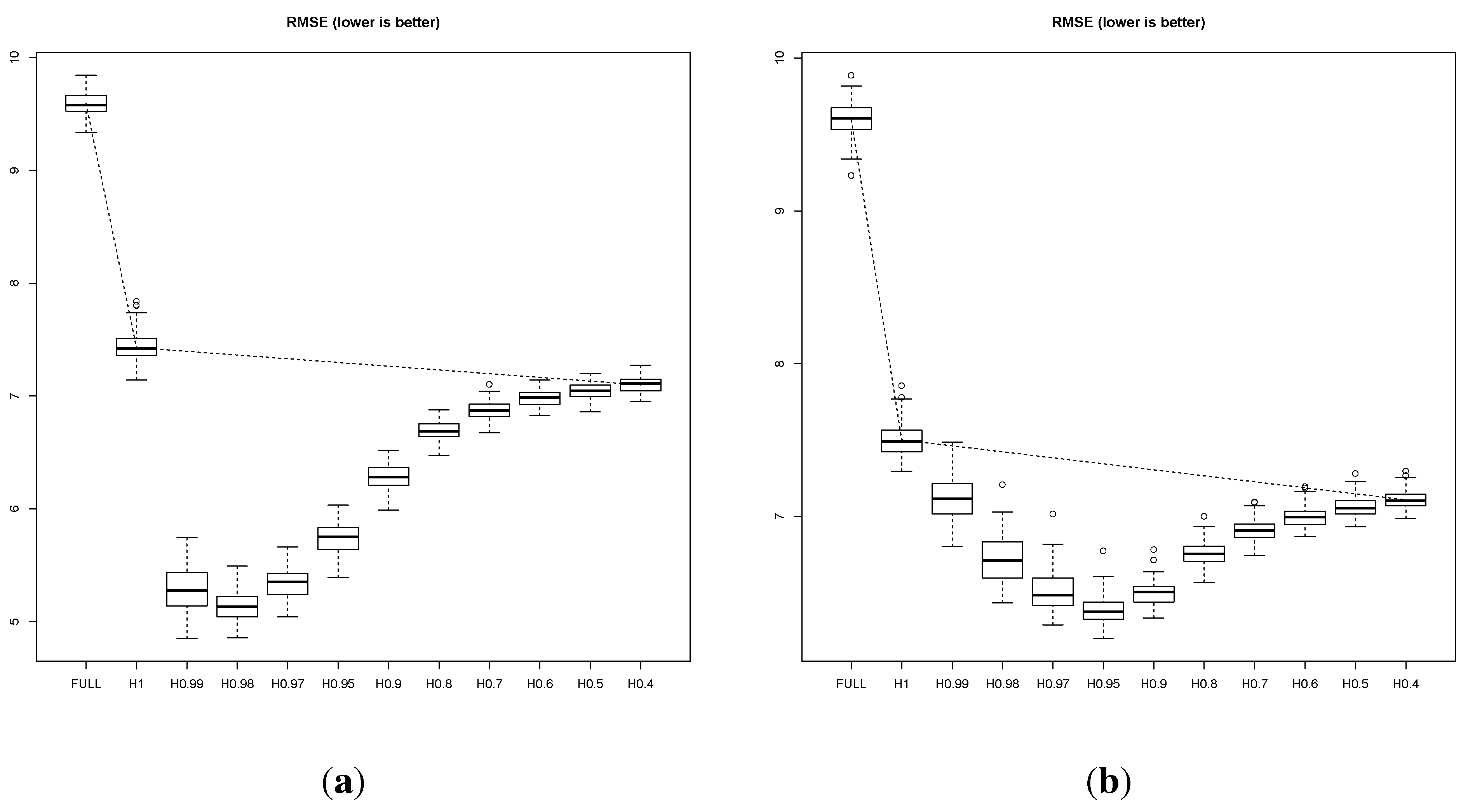
In Figure 4, we plot the one-step-ahead RMSE for a sequence of λ values between $\lambda =1$, where retirement via Bayesian conjugate updating is performed, up to $\lambda =0.4$, where retirement is minimal, and the model effectively discards the data historically. For comparison, we additionally report the performance of a model that is trained using the full data (FULL). There are several interesting points to make. First, we compare the three methods that do not feature exponential forgetting factors: namely, the FULL model; the online model “H1”, that retires discarded points via conjugate Bayesian updating; and the online model “H0.4”, that mostly ignores discarded points and maintains very weakly informative leaf priors. These three setups represent a decreasing reliance on historical information: from fully remembering past data, to remembering them via the leaf priors, to mostly discarding them altogether. A monotonic improvement in performance is observed (note the dotted line connecting the three setups), suggesting that historical information in this context is outright detrimental, and should be altogether ignored. And yet, introducing exponential forgetting at the leaf priors reveals a characteristic U-shaped performance curve, notably lying strictly below the performance attainable by any of the above three methods. The forgetting factor can be seen to negotiate the trade off between throwing away too much information at one extreme ($\lambda =0.4$), and retaining obsolete information at the other ($\lambda =1$). This is emphasized by comparing slow with fast drift: in the former case, $\lambda =0.98$ performs best, whereas $\lambda =0.95$ is the best performer in the latter case. The error bars are tight enough to be confident in this conclusion – although at times neighboring values feature some overlap, the overall shape of the curve is highly statistically significant.

Figure 4. Slowly ($k=0.1$, plot (a)) and rapidly ($k=0.5$, plot (b)) drifting Friedman data experiments. Performance is measured by one-step-ahead RMSE (lower is better) for the FULL model, as well as the online version with various degrees of forgetting, ranging from $\lambda =1$ (no forgetting) to $\lambda =0.4$.

Figure 4. Slowly ($k=0.1$, plot (a)) and rapidly ($k=0.5$, plot (b)) drifting Friedman data experiments. Performance is measured by one-step-ahead RMSE (lower is better) for the FULL model, as well as the online version with various degrees of forgetting, ranging from $\lambda =1$ (no forgetting) to $\lambda =0.4$.

It is worth reiterating that, had we not considered the use of forgetting factors, empirical evidence would have clearly argued in favor of noninformative priors over conjugate priors in drifting contexts, a misguiding conclusion, since in fact “forgetful” conjugate priors, despite their simplicity, represent a major performance improvement. We expect that this result may hold more generally in online Bayesian updating in streaming contexts.

We now turn our attention to model complexity over time. In Figure 5, we investigate the effect that discarding and forgetting have on model complexity, as measured by average tree height over time. A useful aspect of our choice of simulator engine is the fact that as $a_t$ increases in magnitude, the non-linearity of the regression surface will accentuate, as the first term is responsible for much of its complexity. We hence consider an A-B-A regime change setup over a longer time horizon ranging to $t=3\times {10}^4$, setting $a_t=10$ between $t=10,000$ and $t=20,000$ (denoted by vertical lines in Figure 5), and 0 otherwise, so that the complexity of the regression surface rises sharply and then drops again. We deploy a DT without discarding (i.e., sequentially incorporating the full dataset), a DT with a fixed budget of 100 active datapoints and no forgetting, and one with the same budget and mild forgetting ($\lambda =0.9$). First observe that capping the active data pool size significantly penalizes model complexity on the whole, as opposed to maintaining the full dataset in active memory. Also note that all three methods react to the rise in complexity at $t={10}^4$ by favoring deeper trees. However, once the data complexity drops again at $t=2\times {10}^4$, both FULL and H1 retain their average tree depth, failing to return to earlier levels. 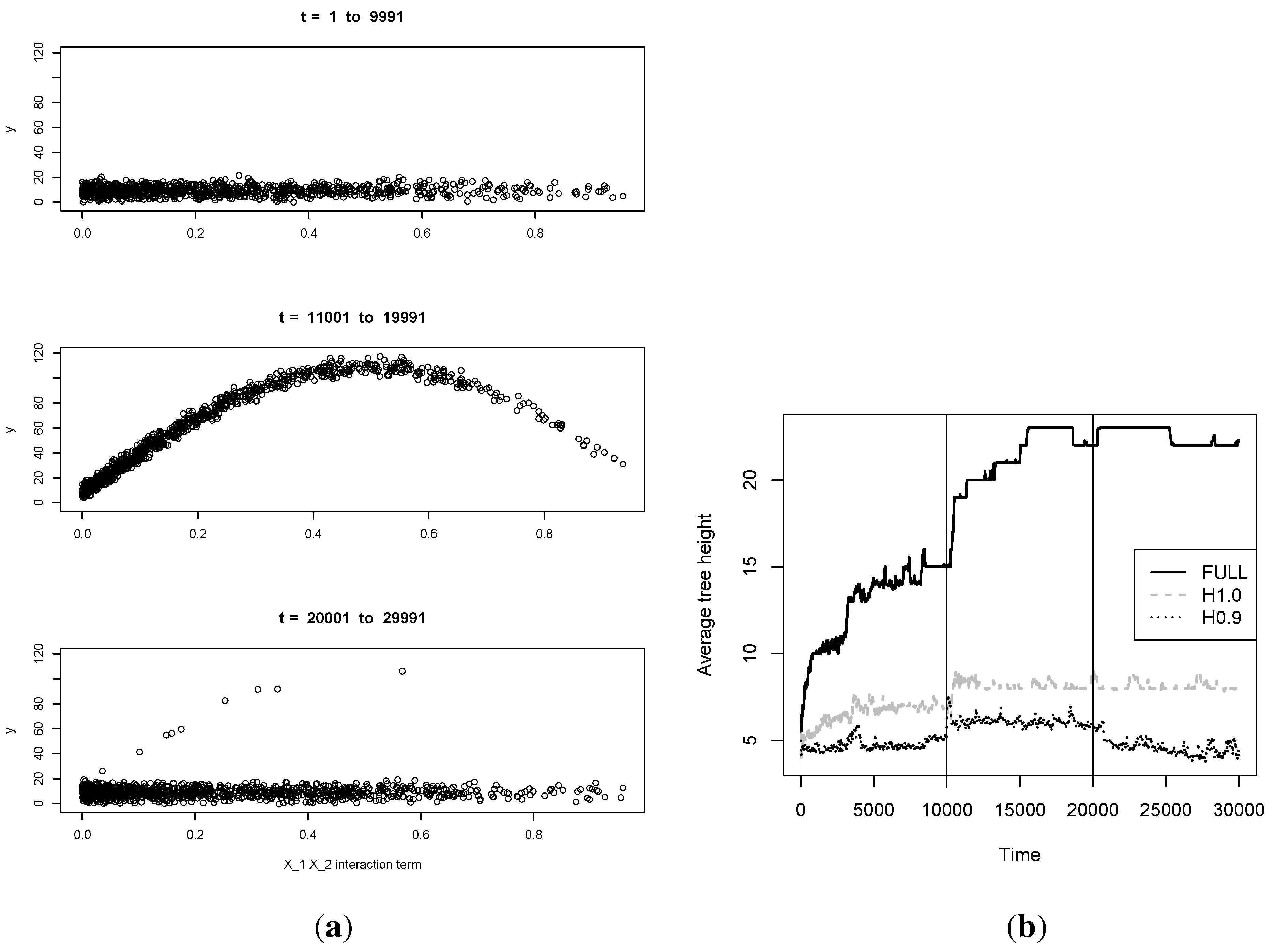By contrast, $\lambda =0.9$ allows the model to adapt to the change and drop its complexity as soon as the data allow it. This difference can be attributed to the fact that without forgetting, leaf priors tend to persist, whereas exponential forgetting allows them to become eventually outweighed by the impact of novel information. Conceptually, since the distant past is increasingly unlike the present, added degrees of freedom are needed to accurately represent both in the same model.

Figure 5. Snapshots of the changing relationship between the response and the interaction term in the Friedman data at various time intervals of the experiment (plot (a)). The true regression surface complexity rises in $t\in [{10}^4,2\times {10}^4]$. The reaction of the average tree height is depicted in plot (b), for FULL, H1, and H0.9.

Figure 5. Snapshots of the changing relationship between the response and the interaction term in the Friedman data at various time intervals of the experiment (plot (a)). The true regression surface complexity rises in $t\in [{10}^4,2\times {10}^4]$. The reaction of the average tree height is depicted in plot (b), for FULL, H1, and H0.9.

5.2. Streaming Classification

We now turn to streaming classification. We again adopt the one-step-ahead performance paradigm, using aggregate measures of classification performance to avoid issues resulting from imbalanced classes, namely the AUC, and a recently proposed alternative, the H-measure [36]. Throughout, we compare with alternative classifiers, to give a balanced view of performance. Please note that this is not intended as an exhaustive comparative study, since not all relevant methods were publicly available or directly applicable (e.g., CVFDT does not support real-valued covariates). We have compared against LDA-AF [12], a streaming linear parametric classifier that claims very stable long-term performance; and random forests [37] implemented over a sliding window (for lack of a more principled streaming version thereof in the literature), where the window size is set to be equal to the active data pool, namely $w=500$. We will look at two datasets, one real and one synthetic, both of length $n=100,000$. We deploy three versions of dynamic trees: “FULL ($n=30\times {10}^3$)” where 30K datapoints are incrementally incorporated without retirement, and no update occurs thereafter; “H1.0”, “H0.5” and “H0.01”, with historical retirement as before.

We start by considering a synthetic dataset, designed to produce a non-linear decision boundary, via an XOR problem that rotates in space over time so that older data become increasingly misleading, referred to as MOVINGXOR, of length $n=100\times {10}^3$. In Figure 6 (left) we show how classification performance evolves over time in terms of AUC measured over a sliding window. The overall performance in terms of both AUC and the H-measure is shown in the leftmost column of Table 2. Data discarding hardly improves performance when $\lambda =1$, whereas for $\lambda =0.5$ significant improvement is possible. 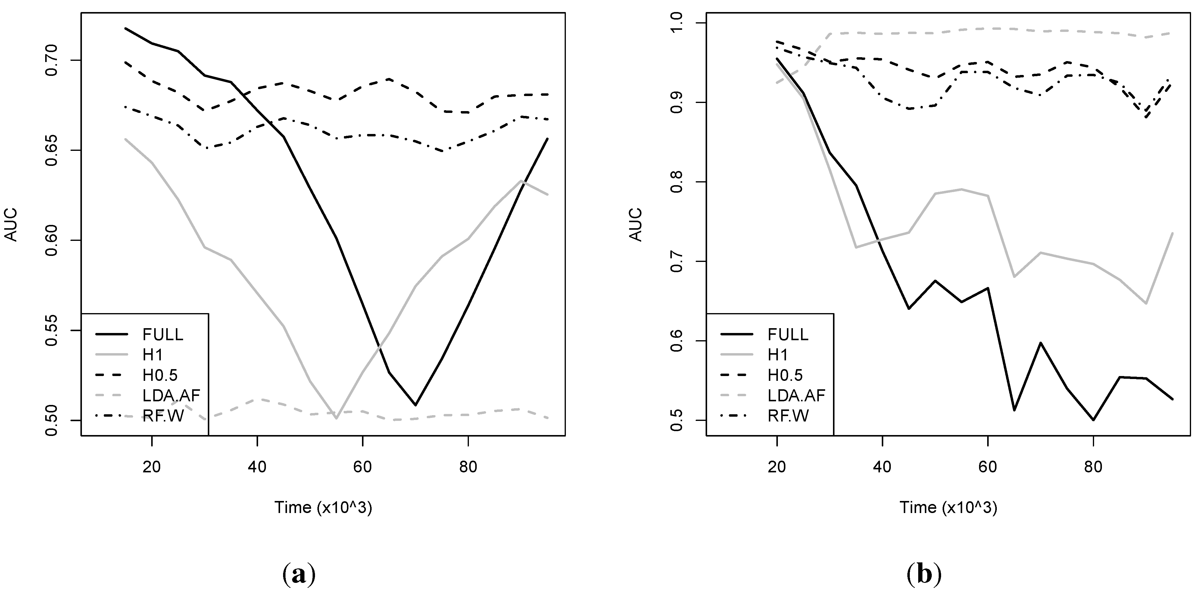In Figure 6, it is visually obvious that this difference is because of the cumulative detrimental effect of obsolete, misleading data which affects both FULL and H1.0 almost equally—their performance only recovering near the end of the simulation where the decision boundary returns to its initial position. RF-W is inferior to H0.5, but stable over time, thanks to the sliding window implementation. In this particular experiment, LDA-AF performs very poorly as expected, given that the true decision boundary is highly non-linear at any given point in time.

Table 2. Overall performance in terms of Area Under the Curve (AUC) and H-measure (H) (in both cases higher is better), for FRAUD and MOVINGXOR.

	MOVINGXOR			FRAUD
	AUC	H		AUC	H
FULL	0.570	0.024		0.661	0.121
H1.0	0.526	0.029		0.805	0.278
H0.5	0.684	0.124		0.952	0.708
LDA.AF	0.504	0.001		0.945	0.748
RF.W	0.662	0.096		0.933	0.710

Table 2. Overall performance in terms of Area Under the Curve (AUC) and H-measure (H) (in both cases higher is better), for FRAUD and MOVINGXOR.

	MOVINGXOR			FRAUD
	AUC	H		AUC	H
FULL	0.570	0.024		0.661	0.121
H1.0	0.526	0.029		0.805	0.278
H0.5	0.684	0.124		0.952	0.708
LDA.AF	0.504	0.001		0.945	0.748
RF.W	0.662	0.096		0.933	0.710

We now consider a real dataset, FRAUD, also of length $n=100\times {10}^3$, containing information about credit card transactions, and their respective status as legitimate or fraudulent, determined by experts (see [12] for more details). An additional challenge with FRAUD is that it is an extremely imbalanced dataset, with the vast majority of examples being non-fraudulent. The presence of drift is again suggested by the deteriorating performance of both H1.0 and FULL over time. Again, H0.5 manages to remain up-to-date and maintain a stable performance, comparable (and slightly superior) to RF-W. Another striking result is that LDA-AF, which was vastly inferior in the synthetic example, dominates here, obtaining an advantage over the best dynamic tree. This result suggests that the true decision boundary is drifting but at any given time remains close to linear. This would put both the DT and RF-W in a disadvantageous position, as trees with constant leaves are not able to easily capture a linear decision boundary. We note however that a DT with linear classification leaves (e.g., logistic regression leaves) is a straightforward extension which we are considering in future work. Note that in terms of overall AUC, H0.5 still outperforms LDA.AF (Table 2). This does not necessarily contradict Figure 6, since aggregate measures of performance such as the AUC or the H-measure perform complex operations over the data, rather than simple averages.

Figure 6. Average classification performance in terms of AUC for the FRAUD dataset (plot (a)) and MOVINGXOR (plot (b)) datasets.

Figure 6. Average classification performance in terms of AUC for the FRAUD dataset (plot (a)) and MOVINGXOR (plot (b)) datasets.

The temptation to produce a “best-performing” method must be balanced against the inescapable fact that the ranking of a classifier will in general depend on the application and the dataset. Still, these experiments give a strong signal that the use of forgetting factors can drastically improve performance of flexible Bayesian tools for online classification in the presence of concept drift, without compromising on coherence or interpretability.

6. Conclusions

In this work, we strive to fully utilize the potential of Bayesian machinery in the context of streaming non-parametrics. We propose data retirement via conjugate Bayesian updating in the context of SMC inference for a dynamic tree model, preserving non-parametric flexibility while enabling constant memory online operation. Second, the availability of tractable predictive distributions allows us to devise computationally efficient active retirement heuristics, hence maintaining a fixed budget of highly informative datapoints. Both features minimize information loss incurred by single-pass processing. Finally, we deploy a maximum entropy heuristic inspired from exponential forgetting factors to introduce temporally adaptive informative priors, and handle concept drift without the need for computationally expensive explicit dynamic modeling. This results in a novel, powerful algorithmic scheme for non-parametric regression and classification tailored to the Big Data era. As future work, we intend to pursue techniques for automatic tuning of forgetting factors in streaming contexts, and their interplay with active retirement heuristics.