1. Introduction
The distribution of carbon dioxide (CO
) in the mid-troposphere is influenced by tropospheric weather and large-scale circulation patterns around the globe and interannual variability associated with the El Niño Southern Oscillation (ENSO) [
1,
2]. Areas with enhanced upward or downward motions associated with large-scale circulations can transport CO
between the free troposphere (FT) and the atmospheric boundary layer (ABL) on the timescale of a day [
3]. If information related to CO
concentrations flows between synoptic systems and the ABL on a daily to subdaily timescale [
3,
4], changes in soil moisture, surface albedo, and temperature that drive biosphere-atmosphere interactions at short timescales may also influence mid-tropospheric CO
. While observations of the vertically integrated CO
mixing ratio have been found to be influenced by continental-scale flux patterns [
5], it is not yet understood how local fluxes from varying land-cover types relate to CO
concentrations in the mid-troposphere.
How is the high-frequency variability of CO
in the ABL communicated to the FT, and how do CO
concentrations in the FT influence CO
concentrations in the ABL? In contrast to ABL CO
concentrations, FT CO
concentrations are governed exclusively by transport mechanisms, either large-scale ascent or descent associated with the Hadley/Walker circulation, other large-scale cells, or baroclinic/synoptic disturbances. Cotton
et al. [
6] quantified “venting" of ABL air into the FT by cloud circulations of different scales and found that synoptic cyclones or mid-latitude baroclinic waves constitute the greatest contribution to ABL venting. One mesoscale modeling study demonstrated that 70% of passive tracers initialized in the boundary layer are transported to the free troposphere over a period of three days [
7]. Sinclair
et al. [
8] attributed this substantial exchange between ABL and FT to the warm conveyor belt, which provides substantial ascent from the ABL to the mid-troposphere. A detailed mass budget demonstrates the ventilation of ABL air into the FT over the warm sector, as well as the entrainment of FT air behind the cold front and near the high-pressure center [
9].
Convective circulations can also promote exchanges between the ABL and FT. Isolated shallow and deep convective cells can ventilate the boundary layer over small areas in the span of a few hours [
10,
11]. Mesoscale convective systems (MCS), complexes of thunderstorms characterized by an organized mesoscale circulation, provide much of the warm-season rainfall over the central U.S. [
12,
13], and these systems contribute substantially to the exchange of air between the ABL and FT [
6]. In the case of MCSs, the exchanges are brought about by individual convective updrafts but also via coherent mesoscale flow structures associated with these systems (e.g., [
14,
15]). Boundary-layer venting from deep convection can also accompany synoptic systems, as in the case of embedded convective elements along a cold front [
16]. Penetrative downdrafts would presumably serve as a means of injecting FT air into the ABL, but this mechanism has not been emphasized in these previous tracer and budget studies.
A recent study examining total column CO
finds that during a frontal system passing over the Park Falls, WI tall tower, CO
concentration above 5 km increased around 5 ppm while drawdown of boundary layer CO
decreased [
5] . These observations confirm that horizontal advection and gradients play a role in total CO
column variation on a subdaily time scale. Advection also influences total CO
column up to seasonal time scales, especially at the onset of the growing season. Keppel-Aleks
et al. [
5,
17] discuss a north-south gradient, which constitutes about a 4 ppm variation between 30
N and 60
N during the growing season, correlated with variations in FT potential temperature.
The concentration of CO
in the ABL is a function of the composition of the original air masses during ABL formation, exchanges with the land surface, and exchanges with the FT as described above, all modulated by variables like land-cover type and soil moisture. Given the role of the inversion as a filter of information between the ABL and the FT, it is important to note the physical processes that affect transport of CO
within the ABL. For example, horizontal transport within the ABL is estimated to move over the land surface at approximately 500 km day
and the surface area influencing the concentration of a trace gas in the ABL, such as CO
, ranges from 10
to 10
km
[
18]. In addition, Cotton
et al. [
6] estimate that vertical transport from convective storm processes around the globe completely replaces the air masses in the ABL approximately 90 times per year, or every four days.
Biological processes affecting CO
concentrations in the ABL include photosynthesis and respiration. Greater surface CO
concentration implies lower levels of photosynthesis and/or higher levels of respiration by plants and microbial communities. Decreased photosynthesis and increased respiration correspond with the end of the growing season and plant senescence or greater microbial activity associated with higher soil moisture and temperature as well as increased leaf litter [
19]. However, on a daily timescale, entrainment of air masses from the FT and vertical transport caused by turbulent fluxes seem to have a greater influence on the early morning temporal evolution of CO
concentration in the ABL than plant uptake from photosynthesis [
20,
21].
Land use and land-management practices also influence vegetation and carbon dynamics within the ABL. Annual burning in grasslands of the Great Plains is practiced in part to control the expansion of invasive species, such as
Cornus drummondii (roughleaf dogwood) and
Juniperus virginiana L. (eastern red cedar). Bremer and Ham [
22] found that controlled annual burning of grasslands increases carbon loss compared with biennial burning, especially at times of above average precipitation. Shrub and tree encroachment leads to increased short-term carbon storage above ground, but these pools are vulnerable to fires and changes in land use. In addition, water availability, vegetation distribution, and rooting depth are important factors in ecosystem carbon dynamics related to woody encroachment [
19,
23].
Variations in photosynthesis and respiration that drive the larger amplitude of diurnal and seasonal carbon cycles associated with vegetation growth and senescence within the ABL are captured by eddy covariance (EC) tower measurements [
24]. In an effort to advance studies of carbon dynamics, national and international observatory networks, such as AmeriFlux, FLUXNET, and the National Ecological Observatory Network, Inc. (NEON), have been established to combine local surface measurements from over 400 EC towers worldwide [
24]. Though the average footprint of towers is on the order of 1 km
, these surface measurements have been used to up-scale CO
concentrations and fluxes to provide estimates of gross primary productivity (GPP) and net ecosystem exchange (NEE) on regional to continental scales [
25,
26]. Estimations of NEE obtained through various “top-down" and “bottom-up" approaches remain restricted by the lack of theoretical knowledge in scaling nonlinear processes related to ecosystem fluxes [
27,
28].
Comparisons of surface and atmospheric measurements are key to understanding CO concentrations and flux dynamics within heterogeneous landscapes and complex, nonlinear processes related to carbon cycling and climate change. Satellite measurements of atmospheric CO concentrations from instruments such as the Atmospheric Infrared Sounder (AIRS) need to be evaluated in relation to ecosystem fluxes to improve assessments of NEE on varying spatial scales. To uncover the relationship between CO concentrations in the mid-troposphere and at the surface, this study asks the questions: How are temporal scales of CO in the mid-troposphere related to surface CO fluxes in a complex, regional landscape, such as grasslands with woody encroachment in northeastern Kansas? And, to what extent can mid-tropospheric CO concentrations be used as a proxy for ABL CO behavior? The goals of this comparative study are to identify the dominant temporal scales of ABL-FT exchange of CO in this region and to assess the utility of AIRS mid-tropospheric CO measurements for illustrating local to regional source/sink dynamics.
To examine whether and when AIRS CO
measurements in the mid-troposphere can be used as a proxy for concentrations at the land surface below, three EC towers were selected at sites with different land-cover types in northeastern Kansas. An information theory approach combining relative entropy and wavelet multi-resolution analysis was used to examine temporal dynamics between AIRS and EC time series of CO
concentrations [
29]. Relative entropy, defined by Vedral [
30] as an “uncertainty deficit," can be a useful measure to improve our understanding of information flow, gain, and transfer in land-atmosphere interactions [
29,
31]. In this study, the methodology combining wavelet multi-resolution analysis with relative entropy allows us to identify the temporal scales where there is the greatest similarity or the least divergence between the probability density functions of AIRS and EC time series of CO
concentrations in the mid-troposphere and at the surface.
3. Results
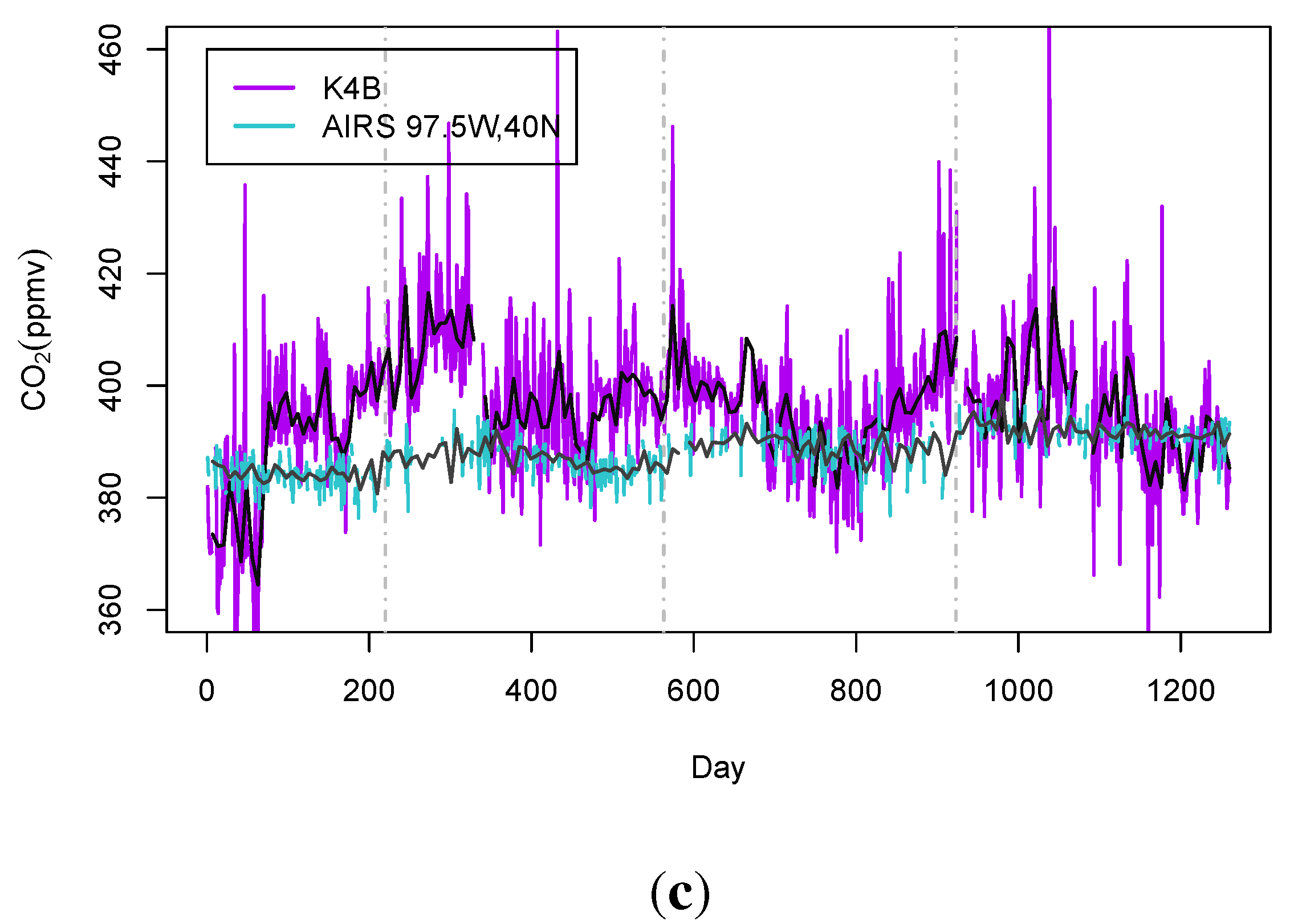
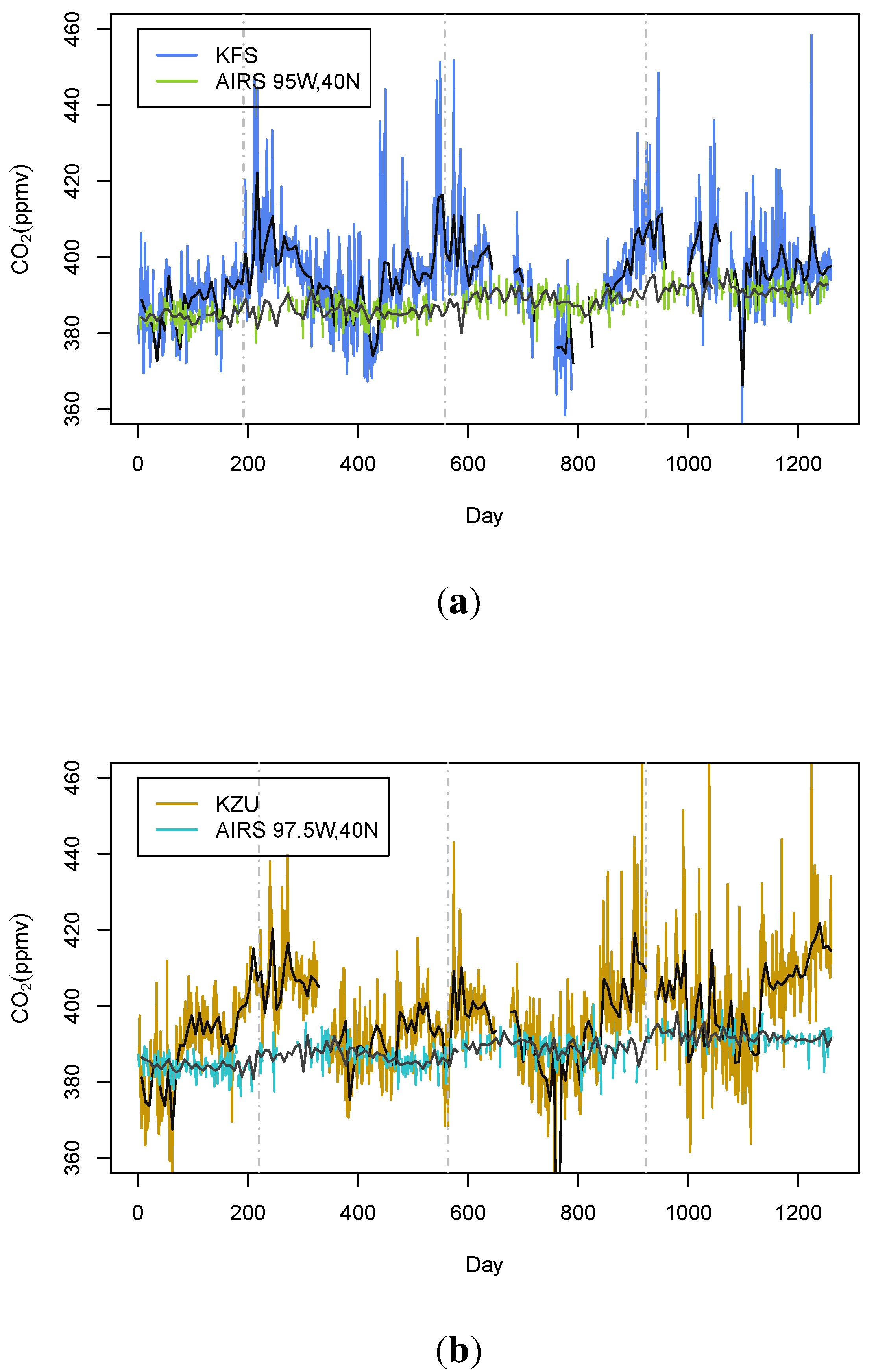
Original, daily time series of surface EC tower measurements and mid-tropospheric AIRS observations of CO
concentration from 2007 to 2010 over KFS, KZU, and K4B are shown in
Figure 1. Brunsell
et al. [
42] have shown that, neglecting CO
released during burning regimes when towers are turned off, all three EC sites are net carbon sinks. AIRS time series exhibit less amplitude and seasonal variation in CO
concentrations than EC tower time series. Despite high missing daily values in the original AIRS time series, a linear regression of weekly averages of the AIRS time series follows the increasing global trend in atmospheric CO
concentrations from approximately 384 ppmv in 2007 to approximately 394 ppmv in 2010.
Figure 1.
Time series of surface EC tower and mid-tropospheric AIRS observations of CO concentration from 2007 to 2010 over (a) KFS; (b) KZU; and (c) K4B. In all panels, the black line indicates the weekly mean of the EC time series and the dark gray line indicates the weekly mean of the AIRS tower time series.
Root mean square error (RMSE) values between the original AIRS and EC time series show a difference of 12.9 ppmv at KFS, 18.9 ppmv at KZU, and 13.9 ppmv at K4B. Once the missing values in the time series have been replaced with the mean of each time series, the RMSE values increase to 13.9 ppmv at KFS, decrease slightly to 18.8 ppmv at KZU, and increase to 14.2 ppmv at K4B. Bias calculations show that AIRS mid-tropospheric observations exhibit a difference from surface measurements of −2.1 ppmv at KFS, −3.0 ppmv at KZU, and −3.2 ppmv at K4B before replacing missing daily values. After replacing the missing values with the mean of each time series, these biases increase to −7.6 ppmv at KFS, −8.8 ppmv at KZU, and −8.3 ppmv at K4B. The RMSE values and bias calculations indicate that site KFS and the corresponding AIRS pixel have the least difference in CO concentration values. Filling missing data values increases the RMSE the most at KFS and bias calculations show an additional difference of at least 5 ppmv at all sites.
Correlations of the original time series and wavelet decompositions of the fields at each temporal scale (
Figure 2) indicate that the greatest positive correlations between surface CO
and mid-tropospheric measurements occurs at the 512-day timescale. At correlation coefficients of 0.2 and above, wavelet decomposed versions of EC time series compared with the original AIRS time series of the corresponding pixels (
Figure 2a) show that the KZU site best reflects AIRS mid-tropospheric CO
concentrations on a 512-day scale compared with sites KFS and K4B. The reverse relationship, where wavelet decomposed versions of AIRS are compared with the original EC time series, also highlights the 512-day scale at which mid-tropospheric CO
may be exchanged with the land surface at the KZU site (
Figure 2b).
Comparing wavelet decomposed versions of both EC and AIRS time series (
Figure 2c) reveals scales of greater contribution between surface and mid-tropospheric CO
exchanges. Stronger positive correlations exist at the 128-day (0.25), 256-day (0.44), and 512-day (0.61) scales for site KFS; at the 16-day (0.25) and 64-day (0.25) scales for site KZU; and at the 512-day (0.28) scale for K4B. Stronger negative correlations are seen at KFS at the 64-day (−0.43) scale, and at K4B at the 64-day (−0.41), 128-day (−0.20), and 256-day (−0.29) scales. The very strong positive correlation (0.99) seen at the 512-day scale for site KZU is indicative of the lower reliability of longer timescales in wavelet multi-resolution analysis [
43,
44], especially when both time series are decomposed.
Figure 2.
Correlations of (a) AIRS time series with wavelet decomposed versions of EC time series; (b) EC time series with wavelet decomposed versions of AIRS time series; and (c) wavelet decomposed versions of EC with wavelet decomposed versions of AIRS. Though wavelets are decomposed to ten temporal scales, only nine (corresponding to 2, 4, 8, 16, 32, 64, 128, 256, and 512 days) are shown here.
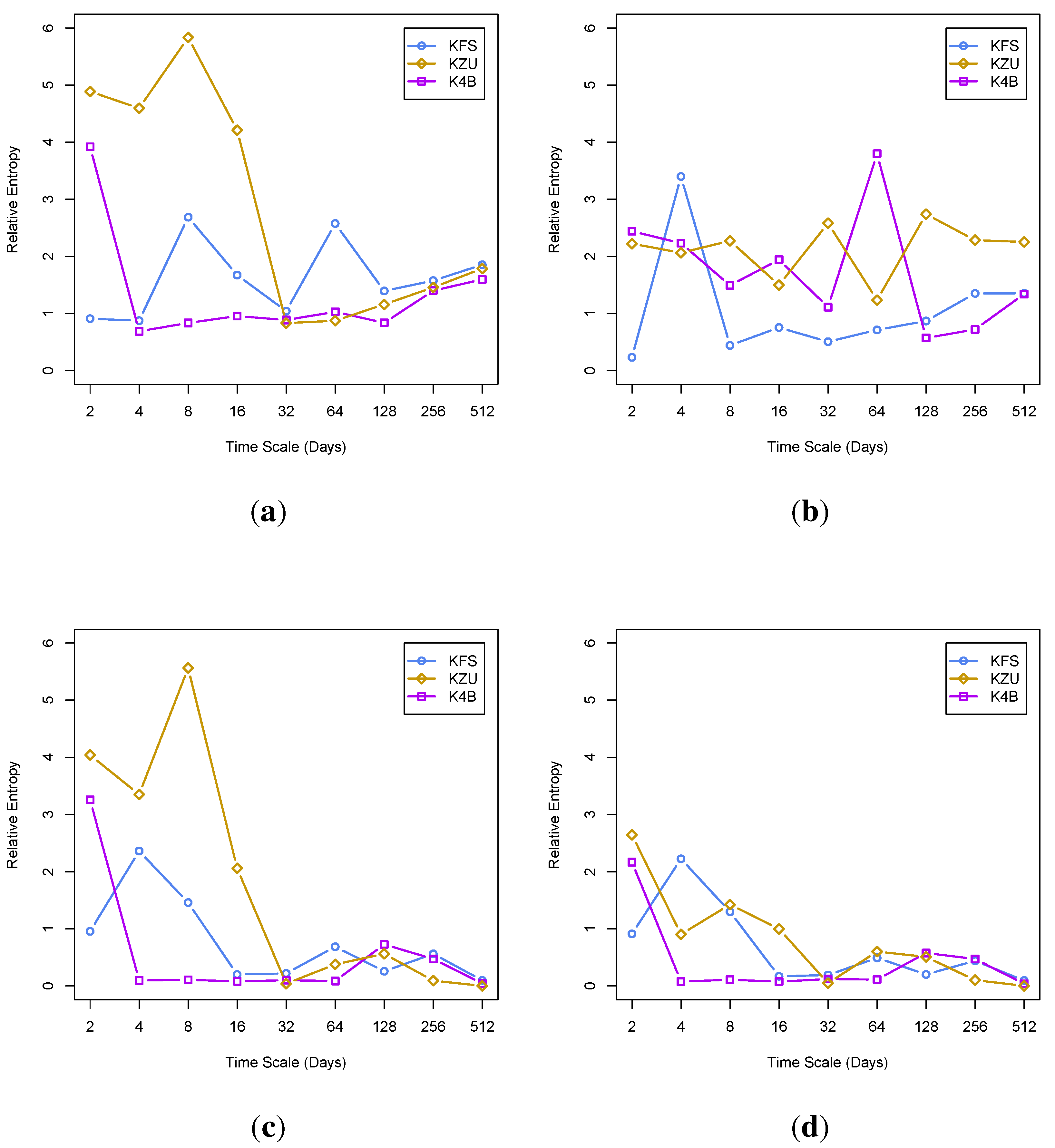
Relative entropy (
R) of wavelet decomposed versions of the EC time series compared with the original AIRS time series, wavelet decomposed versions of the AIRS time series compared with the original EC time series, and wavelet decomposed versions of both AIRS and EC time series are shown in
Figure 3. Lower relative entropy values correspond to greater similarity between the pdfs of the time series,
i.e., less additional information is needed to capture the observed pdf. The timescale for which surface CO
concentrations are closest to the corresponding mid-tropospheric AIRS pixel varies between sites (
Figure 3a). Site KFS shows the least divergence at the four-day scale (
R = 0.88), while site KZU shows the least divergence at timescales of 32 days (
R = 0.81) and 64 days (
R = 0.84). K4B shows the least divergence to mid-tropospheric concentrations at the four-day to the 512-day scale, with lowest
R values occurring at the four-day (
R = 0.66), eight-day (
R = 0.84), and 128-day (
R = 0.83) scales.
Figure 3.
Relative entropy of (a) AIRS time series with wavelet decomposed versions of EC time series; (b) EC time series with wavelet decomposed versions of AIRS time series; (c) wavelet decomposed versions of AIRS with wavelet decomposed versions of EC; and (d) wavelet decomposed versions of EC with wavelet decomposed versions of AIRS. Lower relative entropy corresponds to less divergence or greater similarity between time series.
When assessing how close mid-tropospheric concentrations are to original surface EC measurements (
Figure 3b), the KFS site stands out as being similar to mid-tropospheric CO
at all but the four-day timescale. The least divergence between mid-tropospheric CO
and KFS is seen at the two-day (
R = 0.14) and eight-day (
R = 0.44) scales, and the 16- to 512-day scales also have low
R values. The lowest
R values at the KZU site are seen at timescales of 16 days (
R = 1.48) and 64 days (
R = 1.22). The timescales of least divergence for the K4B site occur at 128 days (
R = 0.52) and 256 days (
R = 0.68), though
R is also low at the 32- and 512-day scales.
To evaluate
R between wavelet decomposed versions of both AIRS and EC time series (
Figure 3c, d), the distances from pdfs of one decomposed series at a particular timescale to the pdfs of the other series at the same timescale are considered. When the distance from the pdf of the decomposed EC time series to the pdf of the decomposed AIRS time series is measured (
Figure 3c), KFS shows the greatest similarity or least divergence from the 16-day (
R = 0.20) to the 512-day (
R = 0.10) scales; KZU shows the greatest similarity or least divergence from the 32-day (
R = 0.04) to the 512-day (
R = 0.003) scales; and K4B shows the greatest similarity or least divergence from the 4-day (
R = 0.10) to the 512-day (
R = 0.04) scales. This pattern of timescales is reflected for all sites in
Figure 3d, where the distance from the pdf of the decomposed AIRS time series to the pdf of the decomposed EC time series is measured. In general, all values of
R are lower when comparing series that are both decomposed.
4. Discussion
Information related to CO
concentration flows both to and from the land surface [
4,
45]. The original AIRS and EC time series show that the global signal of CO
concentrations in the mid-troposphere exhibits less amplitude or variation on daily to annual scales than surface concentrations (
Figure 1). This finding is supported by Maddy
et al. [
39] and can be explained by the different processes governing the diurnal variability of CO
at the surface versus those operating between the ABL and the free troposphere (FT) to influence concentrations in the mid-troposphere [
3,
20].
Using an information theory-based relative entropy approach combined with wavelet multi-resolution analysis, we have identified the dominant temporal scales of ABL-FT exchange of CO and of AIRS utility for revealing source/sink dynamics in this region. While correlations of the wavelet multi-resolution analysis show agreement for all sites on the 512-day timescale, the addition of relative entropy gives insight into similarities on shorter timescales. Results from relative entropy indicate that AIRS could be used as a proxy for all land cover types on the 32-day (monthly) and longer timescales. For land cover types experiencing woody encroachment like KFS and K4B, AIRS may be representative of CO concentrations at shorter timescales depending on how we interpret the influences of site characterization and errors associated with missing daily values.
According to the wavelet multi-resolution analysis, the highest positive correlations between mid-tropospheric and surface CO
concentrations occur at 256 days for site KFS and at 512 days for sites KFS, KZU, and K4B (
Figure 2). While correlations at the 512-day may be influenced by lower reliability at longer timescales in wavelet multi-resolution analysis [
43,
44], it is not surprising that surface and mid-tropospheric CO
concentrations agree on longer timescales when ABL-FT exchanges have become more integrated. The more significant correlations for KZU at the 512-day timescale are most likely related to greater soil respiration found in annually burned grasslands, especially in years of high precipitation, as compared with sites KFS and K4B experiencing woody encroachment [
22]. Ham
et al. [
46] have shown that 85% of respiration in a tallgrass prairie plot, such as KZU, can be attributed to soil respiration. A higher interannual rate of soil respiration makes KZU less of a CO
sink, more closely reflecting the rising global trend seen in the AIRS measurements.
Positive and negative correlations at 64 days in
Figure 2c may illustrate the difference in seasonal dynamics between AIRS and the annually burned site of KZU versus sites KFS and KZU experiencing woody encroachment. Based on the findings of Keppel-Aleks
et al. [
5,
17], the continental-scale gradient of CO
, approximately 4 ppm between 30
N and 60
N, during the growing season may be related to this difference. A multi-month communication lag between ABL CO
and FT concentrations could manifest as a delay between the ABL carbon dynamics accompanying the onset of the growing season and the manifestation of this onset in the FT CO
values. This relationship between AIRS and sites KFS and K4B at the 64-day scale is also evident in the measure of relative entropy (
Figure 3a & b), though the direction of information divergence is seen from KFS to AIRS (
Figure 3a) and from AIRS to K4B (
Figure 3b).
Results of low relative entropy for sites with different land cover types indicate timescales when AIRS is most useful for inferring source/sink dynamics at the surface (
Figure 3a, c). AIRS CO
concentrations diverge least from surface CO
concentrations at site K4B, a lowland area with mixed C
grasses and C
forbs experiencing woody encroachment. Therefore, AIRS may be a good proxy for CO
source/sink dynamics in areas of similar land cover on timescales from 4 to 512 days. On timescales less than a month, AIRS is not a good proxy for annually-burned, C
grasslands like KZU.
On the other hand,
Figure 3b illustrates that the CO
concentrations at KFS closely approximate mid-tropospheric concentrations at all but the four-day timescale. The heterogeneity and land-cover type at the KFS site is perhaps most characteristic of land cover throughout the region. For this reason, it is not surprising that EC tower measurements at KFS are closest to mid-tropospheric concentrations at almost all timescales. Likewise, it is not surprising that CO
concentrations at site KZU, characterized by tallgrass prairie and an annual burn regime, are the least similar with mid-tropospheric concentrations in this region. The large divergence between K4B and AIRS at the 64-day scale may again represent the seasonal differences in CO
concentration at local versus continental scales.
Considering that FT concentrations reflect continental-scale fluxes [
5,
17], it stands to reason that AIRS more closely approximates land covers with woody encroachment versus perennial tallgrass prairie. The land-cover type at site K4B, KFS, and KZU differ through species composition and microclimate. In 2008, for example, the average air temperature at K4B was found to be 0.5
C higher than the other two sites [
32]. Encroachment of
Cornus drummondii or
Juniperus virginiana L. alters soil temperature and microclimate by changing surface albedo. The encroachment of
Juniperus virginiana L. would also mean a change from C
grasses to C
coniferous trees. Analyses of C
and C
plants within a C
-C
mixed grassland on the Konza Prairie have shown that C
plants with greater rooting biomass can be more drought tolerant and continue to photosynthesize beyond C
grasses that are drought stressed [
47].
According to a study conducted on the Konza Prairie by Lett
et al. [
48], carbon storage in aboveground biomass greatly increases with shrub encroachment. Deeply rooted clonal shrub islands of
Cornus drummondii, characteristic of site K4B, were found to have increased from 0 to 18.5% in Konza Prairie sites burned every four years over that last 26 years [
49]. These islands can sequester more than nine times the amount of carbon aboveground compared with open grasslands like KZU [
48]. A shift in plant biomass from belowground to aboveground in areas of woody encroachment may cause short-term carbon sinks, though these are more vulnerable to fire and sequester less carbon as woody plants mature. In a complementary Konza Prairie study, annual soil CO
flux diminished by 16% as grasslands shifted to shrublands [
50].
Juniperus virginiana L. or eastern red cedar is another invasive species found at site K4B that has been shown to alter ecosystem processes by increasing aboveground NPP, litter, and accrual of organic carbon in litter and soil, while decreasing soil respiration [
51].
Various synoptic-scale and mesoscale processes couple concentrations of CO in the ABL and the FT. However, attributing specific mechanisms to the correlations in the wavelet multi-resolution analysis and similarities in relative entropy is a challenge. Mechanisms governing similarities on seasonal timescales (64 to 128 days) are most obvious and straightforward to understand, since the FT CO reflects the growing season over the continent, which is communicated in the vertical by regular occurrences of synoptic systems and deep convection. Relationships at shorter timescales are more difficult to interpret, partly because of the single-point nature of both the EC measurements and the AIRS pixels. A typical EC tower footprint is only 1 km, but we argue that measurements from a single tower are representative of a much larger regional area, given an assumption of the representativeness of the particular land-surface and vegetation properties associated with the EC measurements.
At any given moment, the bulk of the FT is composed of air that recently passed through the ABL [
9], a notion consistent with the four-day cycling timescale estimated by Cotton
et al. [
6]. Similarities between AIRS measurements and both KFS and K4B sites at the four-day scale in
Figure 3a are intriguing. These results may represent shorter-term communication between the ABL and FT via a small number of synoptic or organized convective systems, or they may be an artifact of the data filling process.
Given the RMSE and bias calculations, missing daily values in both the AIRS and EC time series contribute to our results and how we interpret them. Like K4B, KFS is experiencing woody encroachment, but unlike K4B the time series for KFS was originally missing 18.57% of the daily values (
Table 1). Filling the missing data with the same value of the mean from the original time series may influence the results for 8- and 16-day scales shown in
Figure 3a. If we disregard the higher relative entropy values for KFS at the 8- and 16-day scales, we could conclude that AIRS is also a good proxy for land-cover similar to KFS. In addition, the filling for the AIRS time series may influence the high relative entropy value on the four-day scale when the wavelet decomposed version of AIRS is compared with the original KFS signal shown in
Figure 3b.

