Outer Synchronization between Fractional-Order Complex Networks: A Non-Fragile Observer-based Control Scheme

Abstract

This paper addresses the global outer synchronization problem between two fractional-order complex networks coupled in a drive-response configuration. In particular, for a given fractional-order complex network composed of Lur’e systems, an observer-type response network with non-fragile output feedback controllers is constructed. Both additive and multiplicative uncertainties that perturb the control gain matrices are considered. Then, using the stability theory of fractional-order systems and eigenvalue distribution of the Kronecker sum of matrices, we establish some sufficient conditions for global outer synchronization. Interestingly, the developed results are cast in the format of linear matrix inequalities (LMIs), which can be efficiently solved via the MATLAB LMI Control Toolbox. Finally, numerical simulations on fractional-order networks with nearest-neighbor and small-world topologies are given to support the theoretical analysis.

1. Introduction

Most real systems in nature, society and engineering can be properly described by models of complex networks of interacting dynamical units with diverse topologies [1]. In complex networks, various collective behaviors can emerge through the interaction of the units, among which synchronization represents one of the most interesting ones. Since the first observation of synchronization phenomenon of two pendulum clocks by Huygens in 1665, this phenomenon has been discovered in many biological and physical systems, such as pacemaker cells in the heart and nervous systems, synchronously flashing fireflies, networks of neurons in the circadian pacemaker [2,3]. Another topic that is closely related to the synchronization of complex networks is the consensus of multi-agent systems, which means that a team of agents reaches an agreement on certain quantities of interest through local communication. The study of consensus problem not only helps us understand natural phenomena (e.g., schooling of fish, flocking of birds and swarming of bees), but also has a variety of engineering applications (e.g., cooperative control of unmanned aerial vehicles, rendezvous of mobile robots and communication among sensor networks) [4]. Recently, the relation between synchronization of complex networks and consensus of multi-agent systems has been discussed [5,6]. The past few years have witnessed dramatic advances concerned with synchronization of complex networks and consensus of multi-agent systems (for more details, see [7,8,9,10,11,12,13,14,15,16,17] and references therein).

Notwithstanding the vast technical literature on synchronization, the great majority of research efforts has focused on complex networks of coupled integer-order systems, whose dynamics are described by integer-order differential equations. However, it has been recognized that many physical systems are more suitable to be modeled by fractional-order differential equations (i.e., differential equations involving fractional-order derivatives) rather than the classic integer-order ones [18,19]. Fractional-order derivatives provide an excellent instrument for the description of memory and hereditary properties of various materials and processes. Moreover, they include traditional integer-order derivatives as a special case. In addition, many natural collective behaviors can be explained by the complex networks with fractional-order dynamics: for example, the synchronized motion of agents in fractional circumstances, such as macromolecule fluids and porous media [20,21,22]. Therefore, it is meaningful to study synchronization problem in complex networks of coupled fractional-order systems. For convenience, we here call networks composed of integer-order and fractional-order systems “integer-order complex networks (ICNs)" and “fractional-order complex networks (FCNs)", respectively.

In recent years, synchronization in FCNs has begun to receive research attention within the scientific community [23,24,25,26,27,28], with the first systematic studies on synchronization of FCNs emerging in [29]. A common underlying assumption in the above mentioned literature is that they describe the synchronization behavior inside a single network, which has been termed “inner synchronization". For this case, it has been shown that stability of the synchronized state depends on the details of the underlying network topology. The route to inner synchronization differs from the synchronization taking place between two coupled networks. In the latter case, also known as “outer synchronization", the corresponding nodes of two coupled networks will achieve synchronization [30]. In the real world, there are a great many examples about relationships between different networks, such as the original spreading of infectious diseases between two communities, the balance of beneficial bacteria and pathogenic bacteria in our digestive systems, predator-prey interactions in ecological systems. This shows the great importance and challenge to study the dynamics between two coupled networks.

Despite the fact that some advances have been made for outer synchronization [31,32,33,34,35,36,37,38], these literatures almost exclusively report outer synchronization between coupled ICNs. For outer synchronization between two FCNs, the related research work is just beginning and the only two attempts is the work in [39,40]. In [39], the authors treated outer synchronization problem between two different bidirectionally coupled FCNs. However, the stability condition in that work depends on the eigenvalues of a large system matrix. From the viewpoint of computational complexity, the eigenvalue computation of such large size matrix is difficult and even prohibitive. Another work in [40] considered the robust outer synchronization in a setup consisting of two FCNs coupled unidirectionally by way of an open-plus-closed-loop scheme. Although their approach avoids the need to compute eigenvalues of a large system matrix, the outer synchronization behavior is achieved in the “local” sense, not in the “global” sense. When initial conditions of two FCNs lie far away from each other, the two FCNs in [40] would fail to achieve outer synchronization. Therefore, whether outer synchronization behavior between two FCNs can be achieved globally still remains an open problem, which motivates the research of this work. Another motivation comes from concerns on controller gain variations. In practical applications, uncertainties or inaccuracies do occur in the controller implementation stage due to finite word length, round-off errors in numerical computations and finite resolution measuring instruments [41]. Consequently, even though the designed controllers are robust with respect to system uncertainties, they may be very fragile to their own uncertainties. This brings the so-called non-fragile controller design problem, i.e., how to design a controller such that the controller is insensitive (or resilient) to some uncertainties in its coefficients. To the best of authors’ knowledge, the non-fragile control problem for global outer synchronization in coupled FCNs has never been reported in the literature. The above situation is exactly what concerns and interests us.

The aim of this paper is to discuss the global outer synchronization problem between coupled FCNs by designing appropriate non-fragile controllers. We will first construct two drive-response coupled FCNs from the viewpoint of observer theory. Then, using the stability theory of fractional-order systems and the characteristics of the eigenvalue distribution of Kronecker sum of two matrices, we present a basic theorem for outer synchronization. Based on this basic theorem, two sufficient conditions for outer synchronization in the LMI format are derived for the additive and multiplicative controller gain perturbations, respectively. Finally, the effectiveness and feasibility of the designed control strategy for outer synchronization are demonstrated by numerical simulations on chaotic drive-response FCNs with nearest-neighbor or small-world topologies.

The organization of this work is as follows. In Section 2, the preliminaries and problem statement are introduced. The outer synchronization analysis for two designed coupled FCNs is studied and synchronization criteria are proposed in Section 3. In Section 4, corresponding numerical simulations are presented. Finally, conclusions are drawn in Section 5.

Notations. In the sequel, if not explicitly stated, matrices are assumed to have compatible dimensions for algebraic operations. ${\mathbb{R}}^n$ denotes the n-dimensional Euclidean space, ${\mathbb{R}}^{m\times n}$ is the set of all $m\times n$ real matrices; ${\mathit{I}}_n$ represents the $n\times n$ identity matrix, $\mathit{I}$ means an identity matrix of appropriate order; the shorthand $\mathrm{d}\mathrm{i}\mathrm{a}\mathrm{g}\{\cdots \}$ represents a block diagonal matrix; and the superscript “T" stands for matrix transposition. ${\lambda }_{\mathrm{m}\mathrm{i}\mathrm{n}}\left(\mathit{A}\right)$ and ${\lambda }_{\mathrm{m}\mathrm{a}\mathrm{x}}\left(\mathit{A}\right)$ denote the smallest and the largest eigenvalues of a real symmetric matrix $\mathit{A}$, respectively. The operator $\mathrm{S}\mathrm{y}\mathrm{m}\left(\mathit{A}\right)$ denotes $\mathit{A}+{\mathit{A}}^T$ . The notation $\mathit{P}>0(\ge 0,<0,\le 0)$ means that P is positive (semi-positive, negative, semi-negative) definite, and the symbol ⋆ denotes the elements below the main diagonal of a symmetric block matrix. For $\mathit{A}\in {\mathbb{R}}^{m\times n}$ and $\mathit{B}\in {\mathbb{R}}^{p\times q}$, $\mathit{A}\otimes \mathit{B}\in {\mathbb{R}}^{mn\times pq}$ denotes the Kronecker product of the two matrices.

2. Preliminaries and Network Model

2.1. Basic Concepts and Lemmas

In this section, we first recall some definitions related to fractional-order derivatives that will be used throughout this paper. Note that there are different definitions for fractional derivatives, such as Grünwald–Letnikov, Riemann–Liouville, and Caputo definitions [18]. Here we make use of the following Caputo fractional derivative, because its Laplace transform allows utilization of initial conditions of classical integer-order derivative that has known physical interpretations.

Definition 2.1. 

Let $m-1<\alpha \le m$, with $m\in \mathbb{N}$, the Caputo fractional derivative is defined as

$${\displaystyle D_t^{\alpha }h\left(t\right)=J_t^{m-\alpha }{D}_t^{m}h\left(t\right)=\left\{\begin{array}{cc}& \frac{1}{\Gamma (m-\alpha )}{\int }_0^t{(t-\tau )}^{m-\alpha -1}{h}^{\left(m\right)}\left(\tau \right)d\tau ,\alpha \ne m\hfill \\ & h^{\left(m\right)}\left(t\right),\alpha =m\hfill \end{array}\right.}$$

where $h^{\left(m\right)}\left(t\right)=\frac{d^{m}h\left(t\right)}{d{t}^m}$ is the ordinary derivative of integer order m.

To prove the main results in the next section, we need the following lemmas.

Lemma 2.2 

([42]). For the linear fractional-order system

$${\displaystyle D_t^{\alpha }\mathit{x}\left(t\right)=\mathit{A}\mathit{x}\left(t\right),\mathrm{w}\mathrm{i}\mathrm{t}\mathrm{h}\mathit{x}\left(0\right)={\mathit{x}}_0}$$

(1)

where $0<\alpha <1$, $\mathit{x}\in {\mathbb{R}}^n$ and $\mathit{A}\in {\mathbb{R}}^{n\times n}$. System (1) is asymptotically stable if and only if

$${\displaystyle \left|\mathrm{a}\mathrm{r}\mathrm{g}\left(\mathrm{s}\mathrm{p}\mathrm{e}\mathrm{c}\left(\mathit{A}\right)\right)\right|>\frac{\alpha \pi }{2}}$$

(2)

where $\mathrm{s}\mathrm{p}\mathrm{e}\mathrm{c}\left(\mathit{A}\right)$ is the spectrum of system matrix $\mathit{A}$.

Lemma 2.3 

([43]). Let $\mathit{A}\in {\mathbb{R}}^{n\times n}$ have eigenvalues ${\lambda }_i(1\le i\le n)$, and let $\mathit{B}\in {\mathbb{R}}^{m\times m}$ have eigenvalues ${\mu }_i(1\le i\le m)$. Then the Kronecker sum $\mathit{A}\oplus \mathit{B}\triangleq ({\mathit{I}}_m\otimes \mathit{A})+(\mathit{B}\otimes {\mathit{I}}_n)\in {\mathbb{R}}^{mn\times mn}$ has $mn$ eigenvalues

$${\lambda }_1+{\mu }_1,\cdots ,{\lambda }_1+{\mu }_m,{\lambda }_2+{\mu }_1,\cdots ,{\lambda }_2+{\mu }_m,\cdots ,{\lambda }_n+{\mu }_1,\cdots ,{\lambda }_n+{\mu }_m$$

Lemma 2.4 

([44]). Let $\mathit{A}\in {\mathbb{R}}^{n\times n}$ and $0<\alpha <1$. The fractional-order system $D_{*}^{\alpha }\mathit{x}\left(t\right)=\mathit{A}\mathit{x}\left(t\right)$ is asymptotically stable if and only if there exist two real symmetric positive definite matrices ${\mathit{P}}_{k1}\in {\mathbb{R}}^{n\times n}(k=1,2)$, and two skew-symmetric matrices ${\mathit{P}}_{k2}\in {\mathbb{R}}^{n\times n}(k=1,2)$, such that

$${\displaystyle \sum _{i=1}^2\sum _{j=1}^2\mathrm{S}\mathrm{y}\mathrm{m}\{{\Theta }_{ij}\otimes \left(\mathit{A}{\mathit{P}}_{ij}\right)\}<0}$$

(3)

$${\displaystyle \left[\begin{array}{cc}{\mathit{P}}_{11}& {\mathit{P}}_{12}\\ -{\mathit{P}}_{12}& {\mathit{P}}_{11}\end{array}\right]>0,\left[\begin{array}{cc}{\mathit{P}}_{21}& {\mathit{P}}_{22}\\ -{\mathit{P}}_{22}& {\mathit{P}}_{21}\end{array}\right]>0}$$

(4)

where

$${\displaystyle \begin{array}{cc}\hfill {\Theta }_{11}& =\left[\begin{array}{cc}\mathrm{s}\mathrm{i}\mathrm{n}\theta & -\mathrm{c}\mathrm{o}\mathrm{s}\theta \\ \mathrm{c}\mathrm{o}\mathrm{s}\theta & \mathrm{s}\mathrm{i}\mathrm{n}\theta \end{array}\right],{\Theta }_{12}=\left[\begin{array}{cc}\mathrm{c}\mathrm{o}\mathrm{s}\theta & \mathrm{s}\mathrm{i}\mathrm{n}\theta \\ -\mathrm{s}\mathrm{i}\mathrm{n}\theta & \mathrm{c}\mathrm{o}\mathrm{s}\theta \end{array}\right]\hfill \\ \hfill {\Theta }_{21}& =\left[\begin{array}{cc}\mathrm{s}\mathrm{i}\mathrm{n}\theta & \mathrm{c}\mathrm{o}\mathrm{s}\theta \\ -\mathrm{c}\mathrm{o}\mathrm{s}\theta & \mathrm{s}\mathrm{i}\mathrm{n}\theta \end{array}\right],{\Theta }_{22}=\left[\begin{array}{cc}-\mathrm{c}\mathrm{o}\mathrm{s}\theta & \mathrm{s}\mathrm{i}\mathrm{n}\theta \\ -\mathrm{s}\mathrm{i}\mathrm{n}\theta & -\mathrm{c}\mathrm{o}\mathrm{s}\theta \end{array}\right],\theta =\frac{q\pi }{2}\hfill \end{array}}$$

Lemma 2.5 

([45]). For matrices $\mathit{X}$ and $\mathit{Y}$ with appropriate dimensions, the following inequality holds for $\epsilon >0$

$${\displaystyle {\mathit{X}}^T\mathit{Y}+{\mathit{Y}}^T\mathit{X}<\epsilon {\mathit{X}}^T\mathit{X}+\frac{1}{\epsilon }{\mathit{Y}}^T\mathit{Y}}$$

(5)

Lemma 2.6 

([46]). For a given symmetric matrix $\mathit{S}={\mathit{S}}^T$, the following assertions are equivalent

(1) 

$\mathit{S}=\left[\begin{array}{cc}{\mathit{S}}_{11}& {\mathit{S}}_{12}\\ {\mathit{S}}_{21}& {\mathit{S}}_{22}\end{array}\right]<0$;

(2) 

${\mathit{S}}_{11}<0,{\mathit{S}}_{22}-{\mathit{S}}_{12}^T{\mathit{S}}_{11}^{-1}{\mathit{S}}_{12}<0$;

(3) 

${\mathit{S}}_{22}<0,{\mathit{S}}_{11}-{\mathit{S}}_{12}{\mathit{S}}_{22}^{-1}{\mathit{S}}_{12}^T<0$.

2.2. Network Model

In this paper, we will focus on the outer synchronization problem of two coupled fractional-order complex networks with the drive-response (or master-slave, unidirectional) coupling structure, in which the drive network does not receive any information from the response network.

The drive network with each node being a n-dimensional fractional-order differential system in the form of Lur’e type is described as

$${\displaystyle \begin{array}{cc}\hfill D_t^{\alpha }{\mathit{x}}_i=& \mathit{A}{\mathit{x}}_i+\mathit{f}(\mathit{H}{\mathit{x}}_i,t)+\sum _{j=1}^N{c}_{ij}{\mathit{x}}_j\hfill \\ \hfill y_i=& \mathit{H}{\mathit{x}}_i,i=1,2,\cdots ,N\hfill \end{array}}$$

(6)

where $0<\alpha <1$ is the fractional commensurate order, ${\mathit{x}}_i\in {\mathbb{R}}^n$ and $y_i\in \mathbb{R}$ denote the state and scalar output vectors of the i-th node, respectively. The nonlinear vector-valued function $\mathit{f}(·,·):\mathbb{R}\times \mathbb{R}⟶{\mathbb{R}}^n$ is continuously differentiable. The constant matrix $\mathit{A}\in {\mathbb{R}}^{n\times n}$ combing with $\mathit{f}(·,·)$ describes the dynamics of individual nodes. $\mathit{H}\in {\mathbb{R}}^{1\times n}$ is the observer matrix. The matrix $\mathit{C}=\left(c_{ij}\right)\in {\mathbb{R}}^{N\times N}$ is the outer coupling matrix of the drive network, which denotes the network topology, and is defined as follows: if there is a connection between node i and node j ($i\ne j$), then $c_{ij}=c_{ji}>0$; otherwise, $c_{ij}=c_{ji}=0$ ($j\ne i$), and the diagonal elements of matrix $\mathit{C}$ are defined by $c_{ii}=-{\sum }_{\begin{array}{c}j=1\\ j\ne i\end{array}}^N{c}_{ij},i=1,2,\cdots ,N$. It is noted that the configuration matrix $\mathit{C}$ is symmetric with non-positive real eigenvalues and not necessarily irreducible.

Based on the design idea of observer in the control theory, the response network is described as a nonlinear observer

$${\displaystyle \begin{array}{cc}\hfill D_t^{\alpha }{\widehat{\mathit{x}}}_i=& \mathit{A}{\widehat{\mathit{x}}}_i+\mathit{f}(y_i,t)+\sum _{j=1}^N{c}_{ij}{\widehat{\mathit{x}}}_j+{\mathit{U}}_i(y_i,{\widehat{y}}_i)\hfill \\ \hfill {\widehat{y}}_i=& \mathit{H}{\widehat{\mathit{x}}}_i,i=1,2,\cdots ,N\hfill \end{array}}$$

(7)

where ${\widehat{\mathit{x}}}_i\in {\mathbb{R}}^n$ and ${\widehat{y}}_i\in \mathbb{R}$ denote the state and scalar output vectors of node i of the response network, respectively. $\mathit{A}$, $\mathit{f}(·,·)$, $\mathit{H}$ and $\mathit{C}$ are the same as in system Equation (6). ${\mathit{U}}_i(·,·):\mathbb{R}\times \mathbb{R}⟶{\mathbb{R}}^n$ is the control input to be designed.

Considering the control gain perturbations, the actual implemented control input is assumed to be

$${\displaystyle {\mathit{U}}_i(y_i,{\widehat{y}}_i)=(\mathit{L}+\Delta \mathit{L}\left(t\right))(y_i-{\widehat{y}}_i)}$$

(8)

where $\mathit{L}\in {\mathbb{R}}^n$ is the nominal control gain matrix and the term $\Delta \mathit{L}\left(t\right)$ represents the control gain variations. In this paper, the following two classes of the control gain variations are considered:

Type 1: $\Delta \mathit{L}\left(t\right)$ is with the norm-bounded additive form:

$${\displaystyle \Delta \mathit{L}\left(t\right)={\Delta }_1\left(t\right)={\mathit{M}}_1{\mathit{F}}_1\left(t\right){\mathit{N}}_1}$$

(9)

Type 2: $\Delta \mathit{L}\left(t\right)$ is with the norm-bounded multiplicative form:

$${\displaystyle \Delta \mathit{L}\left(t\right)={\Delta }_2\left(t\right)={\mathit{M}}_2{\mathit{F}}_2\left(t\right){\mathit{N}}_2\mathit{L}}$$

(10)

where ${\mathit{M}}_1$, ${\mathit{N}}_1$, ${\mathit{M}}_2$ and ${\mathit{N}}_2$ are known matrices with appropriate dimensions, ${\mathit{F}}_1\left(t\right)$ and ${\mathit{F}}_2\left(t\right)$ are unknown time-varying matrices satisfying the relation

$${\displaystyle {\mathit{F}}_1\left(t\right){\mathit{F}}_1^T\left(t\right)\le \mathit{I},{\mathit{F}}_2\left(t\right){\mathit{F}}_2^T\left(t\right)\le \mathit{I}}$$

(11)

Let us define the errors of outer synchronization ${\mathit{e}}_i={\mathit{x}}_i-{\widehat{\mathit{x}}}_i$, then the following error dynamics of the outer synchronization can be obtained from Equations (6) and (7):

$${\displaystyle D_t^{\alpha }{\mathit{e}}_i=(\mathit{A}-(\mathit{L}+\Delta \mathit{L})\mathit{H}){\mathit{e}}_i+\sum _{j=1}^N{c}_{ij}{\mathit{e}}_j,i=1,2,\cdots ,N}$$

(12)

In this paper, we aim at establishing computable criteria in the LMI format to find the control gain $\mathit{L}$ such that the coupled fractional-order complex networks Equations (6) and (7) achieve global outer synchronization in the following sense

$${\displaystyle \underset{t\to \infty }{lim}∥{\mathit{e}}_i\left(t\right)∥=\underset{t\to \infty }{lim}∥{\mathit{x}}_i\left(t\right)-{\widehat{\mathit{x}}}_i\left(t\right)∥=0,i=1,2,\cdots ,N}$$

(13)

for any initial conditions ${\mathit{x}}_i\left(0\right)$ and ${\widehat{\mathit{x}}}_i\left(0\right)$, where $\parallel ·\parallel$ refers to the Euclidean norm.

Using the Kronecker product, the error system Equation (12) can be compactly rewritten equivalently as

$${\displaystyle D_t^{\alpha }\mathit{e}=\left({\mathit{I}}_N\otimes {\mathit{A}}_{\mathit{L}}+\mathit{C}\otimes {\mathit{I}}_n\right)\mathit{e}\left(t\right)}$$

(14)

where $\mathit{e}={\left({\mathit{e}}_1^T,{\mathit{e}}_2^T,\cdots ,{\mathit{e}}_N^T\right)}^T\in {\mathit{R}}^{nN}$ and ${\mathit{A}}_{\mathit{L}}=\mathit{A}-(\mathit{L}+\Delta \mathit{L})\mathit{H}$. It is implied from the above representation that the global outer synchronization problem between the FCNs Equations (6) and (7) is converted into an equivalent global asymptotical stability problem of the linear error system Equation (14).

3. Global Outer Synchronization Analysis

From Lemma 2.2, the error system Equation (14) is asymptotically stable if the spectrum of system matrix ${\mathit{I}}_N\otimes {\mathit{A}}_{\mathit{L}}+\mathit{C}\otimes {\mathit{I}}_n$ satisfy the inequality (2). It can been seen that the system matrix ${\mathit{I}}_N\otimes {\mathit{A}}_{\mathit{L}}+\mathit{C}\otimes {\mathit{I}}_n$ is the Kronecker sum of ${\mathit{A}}_{\mathit{L}}$ and $\mathit{C}$, then its eigenvalues can be expressed by the sum of eigenvalues of ${\mathit{A}}_{\mathit{L}}$ and eigenvalues of $\mathit{C}$ using Lemma 2.3. Hence, we obtain the following basic theorem.

Theorem 3.1. 

The fractional-order complex networks Equations (6) and (7) with the designed non-fragile controllers (8) will achieve outer synchronization behavior globally, if the following condition is satisfied

$${\displaystyle |\mathrm{a}\mathrm{r}\mathrm{g}\left(\mathrm{s}\mathrm{p}\mathrm{e}\mathrm{c}\left({\mathit{A}}_{\mathit{L}}\right)\right)|>\frac{\alpha \pi }{2}}$$

(15)

where $\mathrm{s}\mathrm{p}\mathrm{e}\mathrm{c}\left({\mathit{A}}_{\mathit{L}}\right)$ is the spectrum of system matrix ${\mathit{A}}_{\mathit{L}}=\mathit{A}-(\mathit{L}+\Delta \mathit{L})\mathit{H}$.

Remark 3.2. 

The importance of this theorem lies in the fact that it converts the outer synchronization problem between coupled FCNs Equations (6) and (7) into the eigenvalue distribution of the uncertain matrix ${\mathit{A}}_{\mathit{L}}$ with the same dimension as a single node, thereby significantly reducing the computational complexity. In addition, it should be noted that in previous work [40] on outer synchronization of FCNs, the linear error systems are often derived through a suitable linearization of the system’s nonlinear functions. This approach often implies “local” stability of the outer synchronization manifold. However, in many applications, global stability of the outer synchronization manifold is very desirable but difficult to achieve. To circumvent this difficulty, here an observer-based design procedure is performed instead of linearizing approximation of the nonlinear function $\mathit{f}(·,·)$ in Equations (6) and (7). Thus the above proposed condition theoretically guarantees the “global” outer synchronization between FCNs Equations (6) and (7).

Remark 3.3. 

For a given pair $(\mathit{H},\mathit{A})$, whether the observer-type response network Equation (7) synchronizes the drive network Equation (6) globally depends on whether the spectrum of system matrix ${\mathit{A}}_{\mathit{L}}$ satisfies the inequality (15). In case when the control gain $\mathit{L}$ is deterministic without uncertainty, i.e., $\Delta \mathit{L}=0$, the control gain $\mathit{L}\in {\mathbb{R}}^n$ may be chosen such that the inequality (15) is satisfied. As is known from the control theory [47], if the pair $(\mathit{H},\mathit{A})$ is observable, i.e., if $\mathrm{r}\mathrm{a}\mathrm{n}\mathrm{k}[{\mathit{H}}^T,{\mathit{A}}^T{\mathit{H}}^T,\cdots ,{\left({\mathit{A}}^T\right)}^{n-1}{\mathit{H}}^T]=n$, then there exists $\mathit{L}$ providing the matrix ${\mathit{A}}_{\mathit{L}}=\mathit{A}-\mathit{L}\mathit{H}$ with any given eigenvalues. Particularly, all eigenvalues of ${\mathit{A}}_{\mathit{L}}$ can be designed to locate the region defined by inequality (15). For other general pair $(\mathit{H},\mathit{A})$, the control gain $\mathit{L}$ is usually determined through a considerable amount of trial and error. However, with control gain uncertainties (9) or (10), the condition (15) is not easy to be checked because there is infinite number of eigenvalues [48]. To effectively avoid this difficulty, in the following we will develop an LMI-based design method.

Now we are in a position to present an LMI-type solvability condition for the outer synchronization problem of coupled FCNs (6) and (7) with the control gain perturbations (9) or (10).

Theorem 3.4. 

Consider the fractional-order complex networks (6) and (7) with the control gain perturbation ${\Delta }_1\left(t\right)$ in Equation (9). Then the outer synchronization between networks (6) and (7) will be achieved globally, if there exist a constant $\epsilon >0$, a symmetric positive definite matrix $\mathit{P}>0$ and a matrix $\mathit{Q}$, satisfying the following LMI:

$${\displaystyle \left[\begin{array}{cc}\Psi & {\mathit{I}}_2\otimes {\left({\mathit{N}}_1\mathit{H}\mathit{P}\right)}^T\\ \star & -\frac{1}{2}\epsilon \mathit{I}\end{array}\right]<0}$$

(16)

where

$${\displaystyle \begin{array}{cc}\hfill \Psi =& \sum _{i=1}^2\mathrm{S}\mathrm{y}\mathrm{m}\left\{{\Theta }_i\otimes (\mathit{A}\mathit{P}-\mathit{Q})\right\}+2\epsilon \left({\mathit{I}}_2\otimes {\mathit{M}}_1{\mathit{M}}_1^T\right)\hfill \end{array}}$$

with

$${\displaystyle {\Theta }_1=\left[\begin{array}{cc}\mathrm{s}\mathrm{i}\mathrm{n}\theta & -\mathrm{c}\mathrm{o}\mathrm{s}\theta \\ \mathrm{c}\mathrm{o}\mathrm{s}\theta & \mathrm{s}\mathrm{i}\mathrm{n}\theta \end{array}\right],{\Theta }_2=\left[\begin{array}{cc}\mathrm{s}\mathrm{i}\mathrm{n}\theta & \mathrm{c}\mathrm{o}\mathrm{s}\theta \\ -\mathrm{c}\mathrm{o}\mathrm{s}\theta & \mathrm{s}\mathrm{i}\mathrm{n}\theta \end{array}\right],\theta =\frac{\alpha \pi }{2}}$$

Moreover, the non-fragile control gain $\mathit{L}$ is given by

$${\displaystyle \mathit{L}=\mathit{Q}{\mathit{P}}^{-1}{\mathit{H}}^T{\left(\mathit{H}{\mathit{H}}^T\right)}^{-1}}$$

(17)

Proof. Setting ${\mathit{P}}_{11}={\mathit{P}}_{21}=\mathit{P}$, ${\mathit{P}}_{12}={\mathit{P}}_{22}=\mathbf{0}$ in Lemma 2.4, we have that if there exists real symmetric positive definite matrix $\mathit{P}$ such that

$${\displaystyle \sum _{i=1}^2\mathrm{S}\mathrm{y}\mathrm{m}\{{\Theta }_i\otimes \left({\mathit{A}}_{\mathit{L}}\mathit{P}\right)\}<0}$$

(18)

then $|\mathrm{a}\mathrm{r}\mathrm{g}\left(\mathrm{s}\mathrm{p}\mathrm{e}\mathrm{c}\left({\mathit{A}}_{\mathit{L}}\right)\right)|>\frac{\alpha \pi }{2}$, where $spec\left({\mathit{A}}_{\mathit{L}}\right)$ is the spectrum of system matrix ${\mathit{A}}_{\mathit{L}}$.

With ${\mathit{A}}_{\mathit{L}}=\mathit{A}-(\mathit{L}+\Delta \mathit{L})\mathit{H}$, the left hand side of Equation (18) can be rewritten as

$${\displaystyle \begin{array}{cc}\hfill \sum _{i=1}^2\mathrm{S}\mathrm{y}\mathrm{m}\{{\Theta }_i\otimes \left({\mathit{A}}_{\mathit{L}}\mathit{P}\right)\}=& \sum _{i=1}^2\mathrm{S}\mathrm{y}\mathrm{m}\{{\Theta }_i\otimes (\mathit{A}\mathit{P}-\mathit{L}\mathit{H}\mathit{P}-\Delta \mathit{L}\mathit{H}\mathit{P})\}\hfill \\ \hfill =& \sum _{i=1}^2\mathrm{S}\mathrm{y}\mathrm{m}\{{\Theta }_i\otimes (\mathit{A}\mathit{P}-\mathit{L}\mathit{H}\mathit{P})\}+\sum _{i=1}^2\mathrm{S}\mathrm{y}\mathrm{m}\{{\Theta }_i\otimes (-{\mathit{M}}_1{\mathit{F}}_1\left(t\right){\mathit{N}}_1\mathit{H}\mathit{P})\}\hfill \end{array}}$$

(19)

From Equation (11), one has

$${\displaystyle \begin{array}{cc}\hfill ({\mathit{I}}_2\otimes {\mathit{F}}_1){({\mathit{I}}_2\otimes {\mathit{F}}_1)}^T& =({\mathit{I}}_2\otimes {\mathit{F}}_1)({\mathit{I}}_2\otimes {\mathit{F}}_1^T)\hfill \\ & ={\mathit{I}}_2\otimes \left({\mathit{F}}_1{\mathit{F}}_1^T\right)\le \mathit{I}\hfill \end{array}}$$

(20)

By Equation (20) and ${\Theta }_{i1}{\Theta }_{i1}^T={\mathit{I}}_2$, it directly follows from Lemma 2.5 that for any real scalar $\epsilon >0$

$${\displaystyle \begin{array}{cc}& \sum _{i=1}^2\mathrm{S}\mathrm{y}\mathrm{m}\{{\Theta }_i\otimes (-{\mathit{M}}_1{\mathit{F}}_1\left(t\right){\mathit{N}}_1\mathit{H}\mathit{P})\}\hfill \\ \hfill =& \sum _{i=1}^2\mathrm{S}\mathrm{y}\mathrm{m}\{-({\Theta }_i\otimes {\mathit{M}}_1)({\mathit{I}}_2\otimes {\mathit{F}}_1)({\mathit{I}}_2\otimes \left({\mathit{N}}_1\mathit{H}\mathit{P}\right))\}\hfill \\ \hfill \le & \sum _{i=1}^2\left\{\epsilon ({\Theta }_i\otimes {\mathit{M}}_1)({\mathit{I}}_2\otimes {\mathit{F}}_1){({\mathit{I}}_2\otimes {\mathit{F}}_1)}^T{({\Theta }_i\otimes {\mathit{M}}_1)}^T+\frac{1}{\epsilon }{({\mathit{I}}_2\otimes {\mathit{N}}_1\mathit{H}\mathit{P})}^T({\mathit{I}}_2\otimes {\mathit{N}}_1\mathit{H}\mathit{P})\right\}\hfill \\ \hfill \le & 2\epsilon \left({\mathit{I}}_2\otimes {\mathit{M}}_1{\mathit{M}}_1^T\right)+\frac{2}{\epsilon }{({\mathit{I}}_2\otimes {\mathit{N}}_1\mathit{H}\mathit{P})}^T({\mathit{I}}_2\otimes {\mathit{N}}_1\mathit{H}\mathit{P})\hfill \end{array}}$$

(21)

Substituting Equation (21) into Equation (19), one has

$${\displaystyle \begin{array}{cc}\hfill \sum _{i=1}^2\mathrm{S}\mathrm{y}\mathrm{m}\left\{{\Theta }_i\otimes \left({\mathit{A}}_{\mathit{L}}\mathit{P}\right)\right\}=& \sum _{i=1}^2\mathrm{S}\mathrm{y}\mathrm{m}\left\{{\Theta }_i\otimes (\mathit{A}\mathit{P}-\mathit{L}\mathit{H}\mathit{P}-\Delta \mathit{L}\mathit{H}\mathit{P})\right\}\hfill \\ \hfill \le & \sum _{i=1}^2\mathrm{S}\mathrm{y}\mathrm{m}\left\{{\Theta }_i\otimes (\mathit{A}\mathit{P}-\mathit{L}\mathit{H}\mathit{P})\right\}\hfill \\ & +2\epsilon \left({\mathit{I}}_2\otimes {\mathit{M}}_1{\mathit{M}}_1^T\right)+\frac{2}{\epsilon }{({\mathit{I}}_2\otimes {\mathit{N}}_1\mathit{H}\mathit{P})}^T({\mathit{I}}_2\otimes {\mathit{N}}_1\mathit{H}\mathit{P})\hfill \end{array}}$$

(22)

Let

$${\displaystyle \mathit{Q}=\mathit{L}\mathit{H}\mathit{P}}$$

(23)

and following from Equation (22), the inequality Equation (18) holds if

$${\displaystyle \sum _{i=1}^2\mathrm{S}\mathrm{y}\mathrm{m}\left\{{\Theta }_i\otimes (\mathit{A}\mathit{P}-\mathit{Q})\right\}+2\epsilon \left({\mathit{I}}_2\otimes {\mathit{M}}_1{\mathit{M}}_1^T\right)+\frac{2}{\epsilon }{({\mathit{I}}_2\otimes {\mathit{N}}_1\mathit{H}\mathit{P})}^T({\mathit{I}}_2\otimes {\mathit{N}}_1\mathit{H}\mathit{P})<0}$$

(24)

Using Lemma 2.6, it is easily seen that Equation (24) is in turn equivalent to the linear matrix inequality Equation (16), which is the condition stated in the theorem. Therefore, $|\mathrm{a}\mathrm{r}\mathrm{g}\left(\mathrm{s}\mathrm{p}\mathrm{e}\mathrm{c}\left({\mathit{A}}_{\mathit{L}}\right)\right)|>\frac{\alpha \pi }{2}$, which implies that outer synchronization between the fractional-order networks (6) and (7) will occur globally by using Theorem 3.1. This completes the proof.

For the FCNs (6) and (7) with the control gain perturbation defined in Equation (10), we have the following results.

Theorem 3.5. 

Consider the fractional-order complex networks (6) and (7) with the control gain perturbation ${\Delta }_2\left(t\right)$ in Equation (10). Then the outer synchronization between networks (6) and (7) will be achieved globally, if there exist a constant $\epsilon >0$, a symmetric positive definite matrix $\mathit{P}>0$ and a matrix $\mathit{Q}$, satisfying the following LMI:

$${\displaystyle \left[\begin{array}{cc}\Psi & {\mathit{I}}_2\otimes {\left({\mathit{N}}_2\mathit{Q}\right)}^T\\ \star & -\frac{1}{2}\epsilon \mathit{I}\end{array}\right]<0}$$

(25)

where

$${\displaystyle \begin{array}{cc}\hfill \Psi =& \sum _{i=1}^2\mathrm{S}\mathrm{y}\mathrm{m}\left\{{\Theta }_i\otimes (\mathit{A}\mathit{P}-\mathit{Q})\right\}+2\epsilon \left({\mathit{I}}_2\otimes {\mathit{M}}_2{\mathit{M}}_2^T\right)\hfill \end{array}}$$

with

$${\displaystyle {\Theta }_1=\left[\begin{array}{cc}\mathrm{s}\mathrm{i}\mathrm{n}\theta & -\mathrm{c}\mathrm{o}\mathrm{s}\theta \\ \mathrm{c}\mathrm{o}\mathrm{s}\theta & \mathrm{s}\mathrm{i}\mathrm{n}\theta \end{array}\right],{\Theta }_2=\left[\begin{array}{cc}\mathrm{s}\mathrm{i}\mathrm{n}\theta & \mathrm{c}\mathrm{o}\mathrm{s}\theta \\ -\mathrm{c}\mathrm{o}\mathrm{s}\theta & \mathrm{s}\mathrm{i}\mathrm{n}\theta \end{array}\right],\theta =\frac{\alpha \pi }{2}}$$

Moreover, the non-fragile control gain $\mathit{L}$ is given by

$${\displaystyle \mathit{L}=\mathit{Q}{\mathit{P}}^{-1}{\mathit{H}}^T{\left(\mathit{H}{\mathit{H}}^T\right)}^{-1}}$$

(26)

Proof. It is similar to that of Theorem 3.4, the details are then omitted.

A particular case of Theorems 3.4 and 3.5 is $\Delta \mathit{L}=0$. In such a case, we can still provide a sufficient condition for global outer synchronization.

Corollary 3.6. 

Consider the fractional-order complex networks (6) and (7) without the control gain perturbation (i.e., $\Delta \mathit{L}=0$). Then the outer synchronization between networks (6) and (7) will be achieved globally, if there exist a symmetric positive definite matrix $\mathit{P}>0$ and a matrix $\mathit{Q}$, satisfying the following LMI:

$${\displaystyle {\Theta }_1\otimes (\mathit{A}\mathit{P}-\mathit{Q})+{\Theta }_1^T\otimes {(\mathit{A}\mathit{P}-\mathit{Q})}^T+{\Theta }_2\otimes (\mathit{A}\mathit{P}-\mathit{Q})+{\Theta }_2^T\otimes {(\mathit{A}\mathit{P}-\mathit{Q})}^T<0}$$

(27)

where

$${\displaystyle {\Theta }_1=\left[\begin{array}{cc}\mathrm{s}\mathrm{i}\mathrm{n}\theta & -\mathrm{c}\mathrm{o}\mathrm{s}\theta \\ \mathrm{c}\mathrm{o}\mathrm{s}\theta & \mathrm{s}\mathrm{i}\mathrm{n}\theta \end{array}\right],{\Theta }_2=\left[\begin{array}{cc}\mathrm{s}\mathrm{i}\mathrm{n}\theta & \mathrm{c}\mathrm{o}\mathrm{s}\theta \\ -\mathrm{c}\mathrm{o}\mathrm{s}\theta & \mathrm{s}\mathrm{i}\mathrm{n}\theta \end{array}\right],\theta =\frac{\alpha \pi }{2}}$$

Moreover, the non-fragile control gain $\mathit{L}$ is given by

$${\displaystyle \mathit{L}=\mathit{Q}{\mathit{P}}^{-1}{\mathit{H}}^T{\left(\mathit{H}{\mathit{H}}^T\right)}^{-1}}$$

(28)

Proof. It follows directly from Theorems 3.4 and 3.5, and the details are therefore omitted here.

Remark 3.7. 

The above theorems and corollary present sufficient conditions for the solvability of non-fragile outer synchronization problem for coupled fractional-order complex networks, which are related to the solutions to LMIs. In this case, these LMIs can be solved efficiently by resorting to some standard numerical algorithms [46].

4. Numerical Simulations

In this section, numerical examples are given to verify the effectiveness of the above design scheme. For the control gain perturbations in additive form, the coupled fractional-order jerk model based on nearest-neighbor topology is first utilized to demonstrate the main results of Theorem 3.4. Then, a small-world complex network consisted of fractional-order Duffing oscillators is introduced to illustrate the correctness of Theorem 3.5 for the control gain perturbations in multiplicative form.

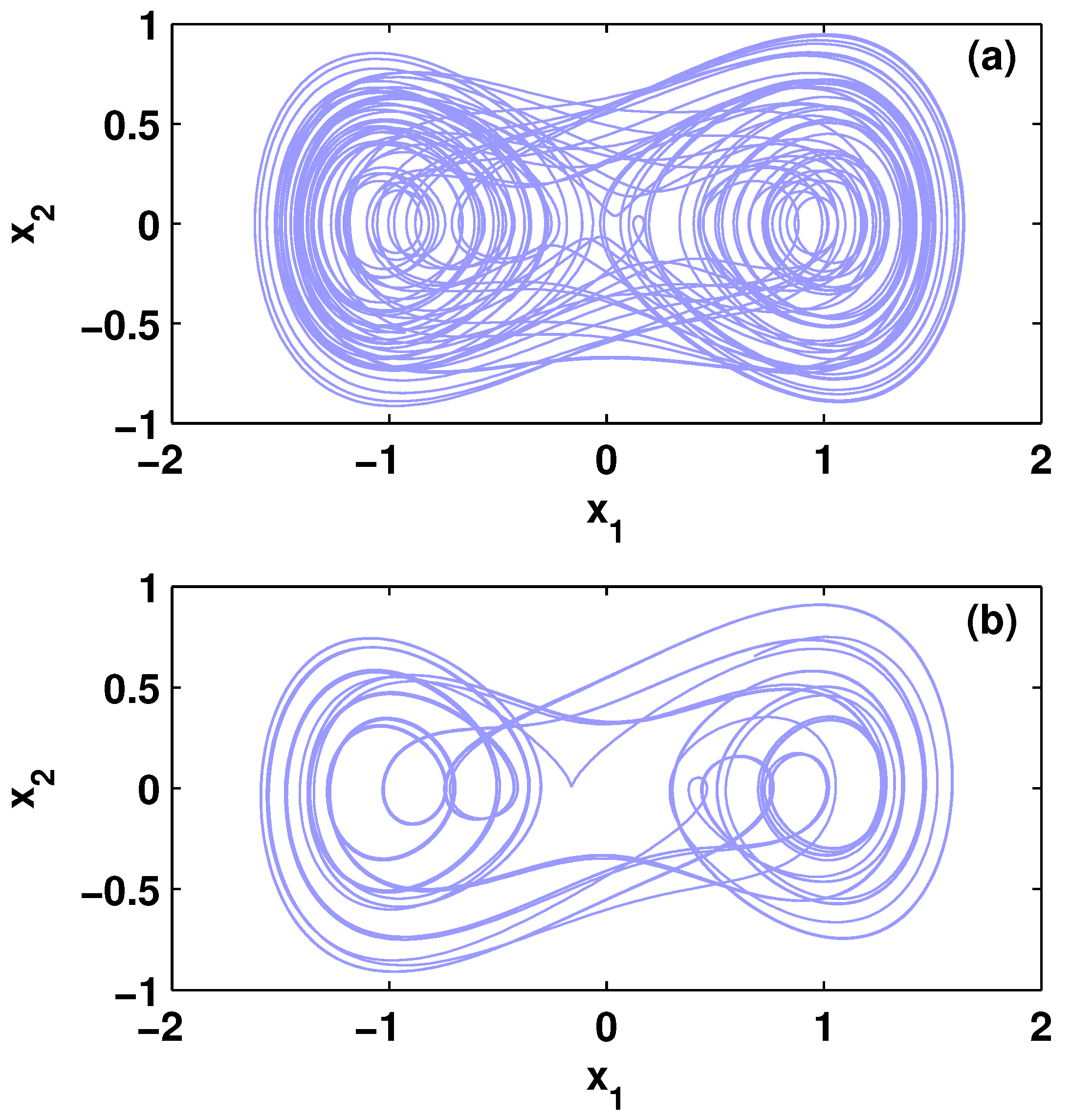
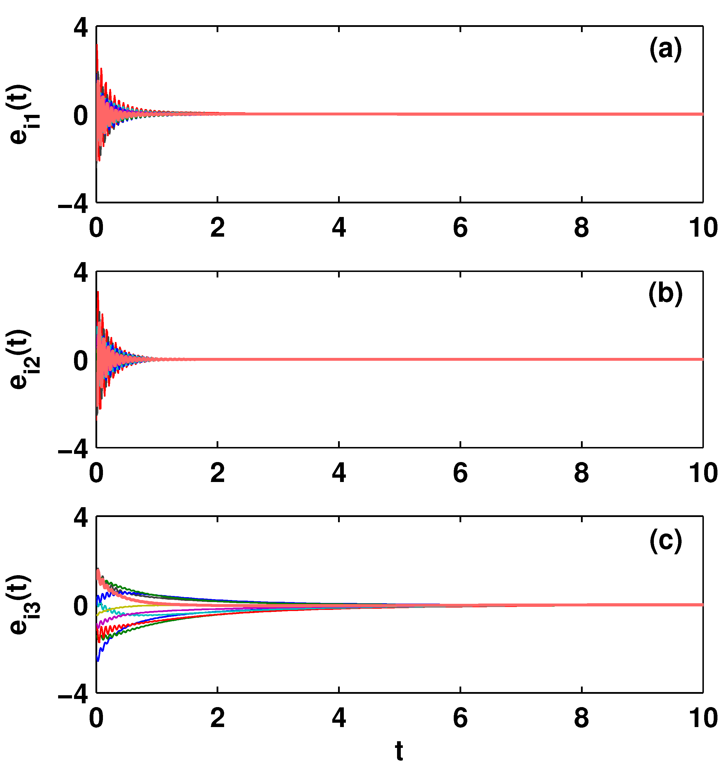
4.1. Outer Synchronization between Two FCNs with Nearest-Neighbor Network Topology

This subsection considers two coupled FCNs with $N=10$ nodes each and nearest-neighbor network topology. The dynamics of the nodes in two networks is determined by the following fractional-order jerk model [49]:

$${\displaystyle \left\{\begin{array}{cc}\hfill D_t^{\alpha }{x}_1& =x_2\hfill \\ \hfill D_t^{\alpha }{x}_2& =x_3\hfill \\ \hfill D_t^{\alpha }{x}_3& =-x_2-\rho x_3+\phi \left(x_1\right)\hfill \end{array}\right.}$$

(29)

with nonlinear characteristic

$${\displaystyle \phi \left(x_1\right)=-1.2x_1+2\mathrm{s}\mathrm{g}\mathrm{n}\left(x_1\right)}$$

and the measured output

$${\displaystyle y\left(t\right)=x_1\left(t\right)}$$

where $x_1$, $x_2$ and $x_3$ are, respectively, the position, velocity, and acceleration of the object, $\rho >0$ is the control parameter. This model in its integer-order version (i.e., $\alpha =1$) is used to determine the time derivative of acceleration of an object and is known to give chaos for $\rho =0.6$. For system (29), we show that the chaotic behavior is preserved in the fractional-order case, as shown in Figure 1 for $\alpha =0.95$. In Lur’e form, the fractional-order jerk model (29) can be represented with

$${\displaystyle \mathit{A}=\left(\begin{array}{ccc}0& 1& 0\\ 0& 0& 1\\ 0& -1& -\rho \end{array}\right),\mathit{f}\left(y\right)=\left(\begin{array}{c}0\\ 0\\ \phi \left(y\right)\end{array}\right),\mathit{H}=(1,0,0)}$$

(30)

The additive control gain perturbations $\Delta \mathit{L}\left(t\right)$ can be described by (9) with

$${\displaystyle {\mathit{M}}_1=\left(\begin{array}{ccc}0.05& -0.13& 0.1\\ -0.24& 0.54& 0.2\\ -0.15& -0.2& 0.16\end{array}\right),{\mathit{F}}_1\left(t\right)=\left(\begin{array}{ccc}\mathrm{c}\mathrm{o}\mathrm{s}\left(3t\right)& 0& 0\\ 0& \mathrm{c}\mathrm{o}\mathrm{s}(0.1t)& 0\\ 0& 0& \mathrm{s}\mathrm{i}\mathrm{n}\left(2t\right)\end{array}\right),{\mathit{N}}_1=\left(\begin{array}{c}0.1\\ 0.2\\ 0.15\end{array}\right)}$$

(31)

For the nearest-neighbor coupling structure, the coupling matrix is given by

$$\mathit{C}=\left(\begin{array}{cccccc}-2k& k& 0& \cdots & 0& k\\ k& -2k& k& 0& \cdots & 0\\ & \ddots & \ddots & \ddots & & \\ 0& \cdots & 0& k& -2k& k\\ k& 0& \cdots & 0& k& -2k\end{array}\right)$$

(32)

where $k>0$ denotes the coupling strength of the whole network.

Figure 1. Chaotic behavior of the fractional-order jerk model (29). The fractional orders are: (a) $\alpha =1$ and (b) $\alpha =0.95$.

Figure 1. Chaotic behavior of the fractional-order jerk model (29). The fractional orders are: (a) $\alpha =1$ and (b) $\alpha =0.95$.

Since the above $\Delta \mathit{L}\left(t\right)$ is in the form of Type 1, Theorem 3.4 is used to design a non-fragile observer-based control (8). Using the MATLAB LMI Control Toolbox, we find that the LMI (16) in Theorem 3.4 is feasible. A feasible solution is presented as follows:

$${\displaystyle \epsilon =85.0407,\mathit{P}=\left(\begin{array}{ccc}41.2019& -0.0000& 0.0000\\ -0.0000& 53.1504& -0.0000\\ 0.0000& -0.0000& 53.1504\end{array}\right),\mathit{Q}={10}^3\times \left(\begin{array}{ccc}0.0146& 2.9380& -0.0124\\ -2.8902& 0.0299& -0.4075\\ 0.0154& 0.4040& -0.0148\end{array}\right)}$$

Therefore, based on the Equation (17) in Theorem 3.4, the nominal control gain is given by:

$${\displaystyle \mathit{L}=\mathit{Q}{\mathit{P}}^{-1}{\mathit{H}}^T{\left(\mathit{H}{\mathit{H}}^T\right)}^{-1}=\left(\begin{array}{c}0.3539\\ -70.1471\\ 0.3734\end{array}\right)}$$

(33)

With the aforementioned control gain matrix and $k=1$, the simulation results for synchronization errors $e_{ij}(i=1,2,\cdots ,10,j=1,2,3)$ of networks (6) and (7) are given in Figure 2, where the initial conditions ${\mathit{x}}_i\left(0\right)$ and ${\widehat{\mathit{x}}}_i\left(0\right)$ are randomly chosen. As seen in Figure 2, the trajectories of the synchronization errors approach zero, which imply outer synchronization between complex networks (6) and (7) with fractional-order jerk models as nodes’ dynamics.

Figure 2. Synchronization errors between the FCNs (6) and (7), where each node is a chaotic fractional-order jerk model (29). (a) The time evolutions of $e_{i1}\left(t\right)=x_{i1}\left(t\right)-{\widehat{x}}_{i1}\left(t\right)$; (b) the time evolutions of $e_{i2}\left(t\right)=x_{i2}\left(t\right)-{\widehat{x}}_{i2}\left(t\right)$; (c) the time evolutions of $e_{i3}\left(t\right)=x_{i3}\left(t\right)-{\widehat{x}}_{i3}\left(t\right)(i=1,2,\cdots ,10)$.

Figure 2. Synchronization errors between the FCNs (6) and (7), where each node is a chaotic fractional-order jerk model (29). (a) The time evolutions of $e_{i1}\left(t\right)=x_{i1}\left(t\right)-{\widehat{x}}_{i1}\left(t\right)$; (b) the time evolutions of $e_{i2}\left(t\right)=x_{i2}\left(t\right)-{\widehat{x}}_{i2}\left(t\right)$; (c) the time evolutions of $e_{i3}\left(t\right)=x_{i3}\left(t\right)-{\widehat{x}}_{i3}\left(t\right)(i=1,2,\cdots ,10)$.

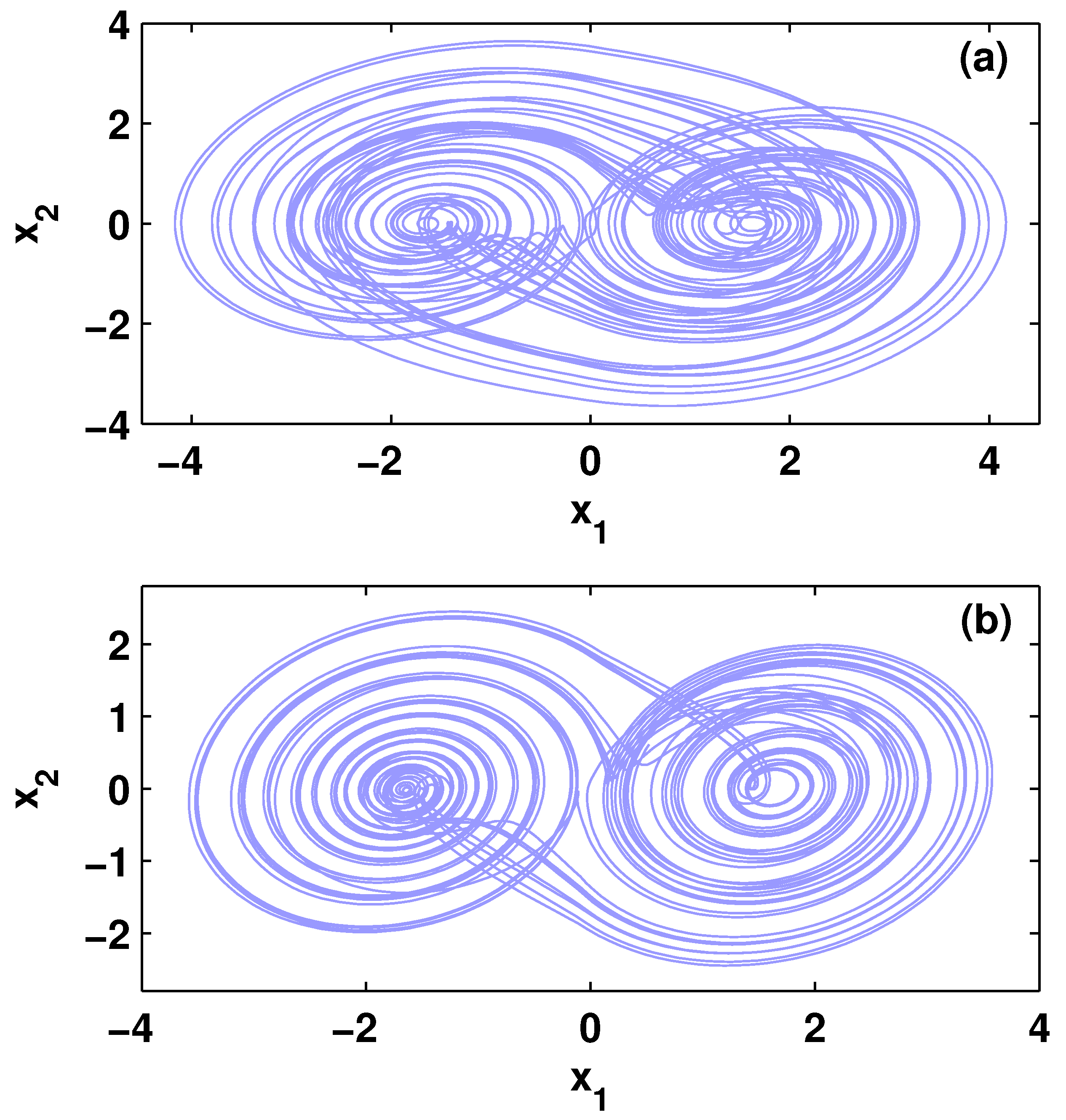
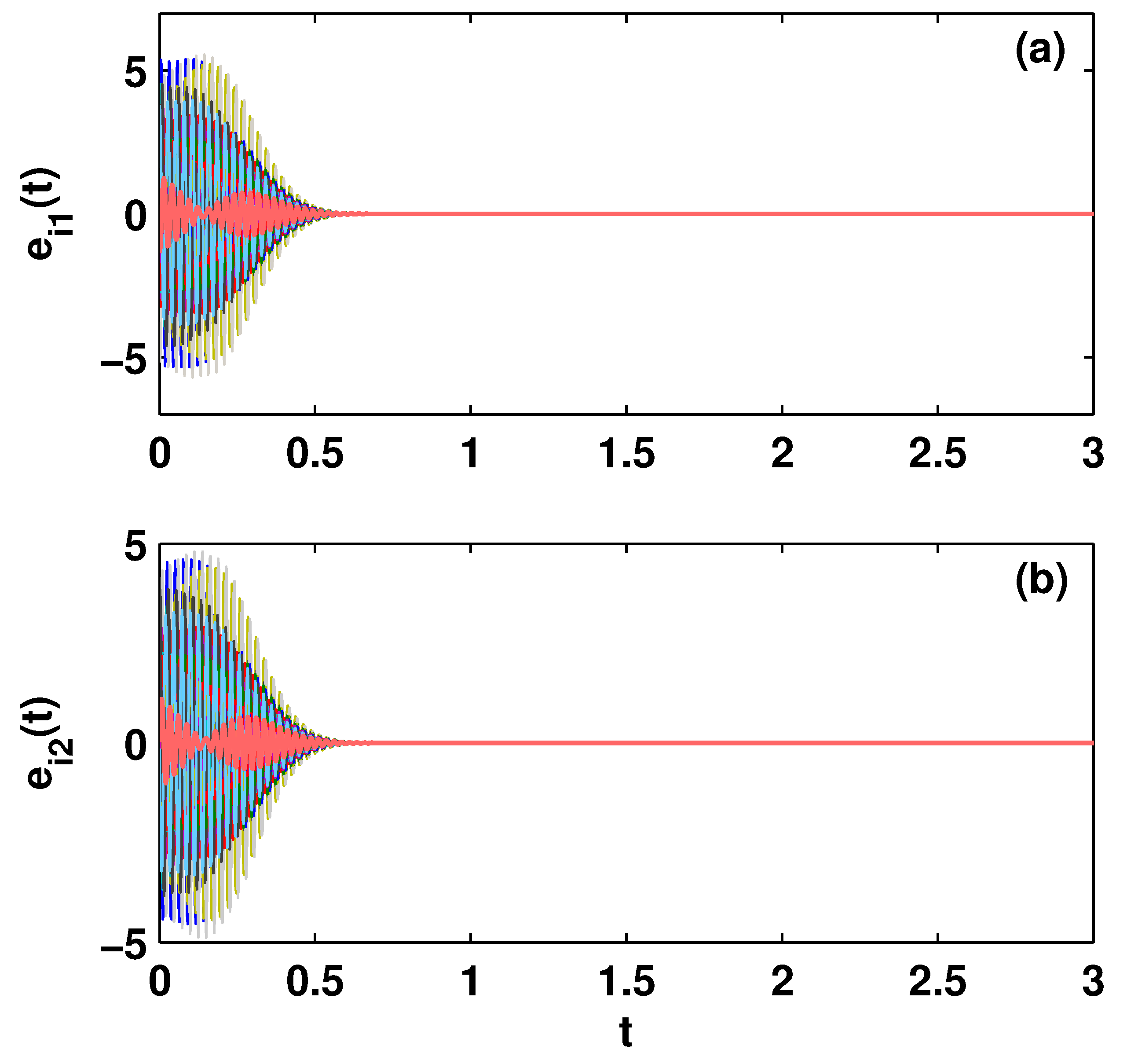
4.2. Outer Synchronization between Two FCNs with Small-World Network Topology

In this simulation, two small-world FCNs of $N=100$ Duffing oscillators are constructed. A single fractional-order Duffing oscillator [50] is described by:

$${\displaystyle \left\{\begin{array}{cc}\hfill D_t^{\alpha }{x}_1& =x_2\hfill \\ \hfill D_t^{\alpha }{x}_2& =-p_1{x}_2-p_2{x}_1-p_3{x}_1^3+q\mathrm{c}\mathrm{o}\mathrm{s}\left(\omega t\right)\hfill \end{array}\right.}$$

(34)

with the measured output

$${\displaystyle y\left(t\right)=\mathit{H}\mathit{x}\left(t\right)=(1,0){(x_1\left(t\right),x_2\left(t\right))}^T}$$

(35)

where $p_1,p_2,p_3$ and q are system parameters. The system can be represented in Lur’e form with

$${\displaystyle \mathit{A}=\left(\begin{array}{cc}0& 1\\ -p_2& -p_1\end{array}\right),\mathit{f}(y,t)=\left(\begin{array}{c}0\\ -p_3{y}^3+q\mathrm{c}\mathrm{o}\mathrm{s}\left(\omega t\right)\end{array}\right)}$$

(36)

For the parameters $p_1=1/25$, $p_2=-1/5$, $p_3=8/15$, $q=2/5$ and $\omega =0.2$, the fractional-order Duffing oscillator (34) exhibits chaotic behavior for $\alpha =0.98$ (see Figure 3).

Figure 3. Chaotic behavior of the fractional-order Duffing oscillator (34). The fractional orders are: (a) $\alpha =1$ and (b) $\alpha =0.98$.

Figure 3. Chaotic behavior of the fractional-order Duffing oscillator (34). The fractional orders are: (a) $\alpha =1$ and (b) $\alpha =0.98$.

The additive controller uncertainties in Equation (10) are considered through

$${\displaystyle {\mathit{M}}_2=\left(\begin{array}{cc}-0.5& -0.24\\ 0.1& -0.35\end{array}\right),{\mathit{F}}_2\left(t\right)=\left(\begin{array}{cc}\mathrm{s}\mathrm{i}\mathrm{n}(0.1t)& 0\\ 0& \mathrm{c}\mathrm{o}\mathrm{s}\left(5t\right)\end{array}\right),{\mathit{N}}_2=\left(\begin{array}{cc}0.2& 0.16\\ -0.05& 0.32\end{array}\right)}$$

(37)

Since the control gain perturbations $\Delta \mathit{L}\left(t\right)$ is in the form of Type 2, Theorem 3.5 is used to design the non-fragile observer-based control (8). Using the MATLAB LMI Control Toolbox, a feasible solution to the LMI (25) in Theorem 3.5 is given by

$${\displaystyle \epsilon =71.6499,\mathit{P}=\left(\begin{array}{cc}40.9209& -1.7321\\ -1.7321& 31.6650\end{array}\right),\mathit{Q}={10}^3\times \left(\begin{array}{cc}0.0212& -7.5497\\ 7.5921& 0.0151\end{array}\right)}$$

Therefore, based on the Equation (26) in Theorem 3.5, the nominal control gain is given by:

$${\displaystyle \mathit{L}=\mathit{Q}{\mathit{P}}^{-1}{\mathit{H}}^T{\left(\mathit{H}{\mathit{H}}^T\right)}^{-1}=\left(\begin{array}{c}-9.5952\\ 185.9816\end{array}\right)}$$

(38)

The zero-row-sum coupling matrix $\mathit{C}$ is generated from the known Watts–Strogatz small-world network model [51] with $N=100$, $m=3$ and $p=0.1$ . According to Theorem 3.5, the outer synchronization between two fractional-order complex networks of coupled Duffing oscillators with small-world topology will be achieved globally. Figure 4 shows the changes in synchronization errors $e_{ij}(i=1,2,\cdots ,100,j=1,2)$, respectively. From these simulation results, it can be seen the designed drive-response networks achieve outer synchronization globally and the effectiveness of the theoretical analysis is demonstrated.

Figure 4. Synchronization errors between the FCNs (6) and (7), where each node is a chaotic fractional-order Duffing oscillator (34). (a) The time evolutions of $e_{i1}\left(t\right)=x_{i1}\left(t\right)-{\widehat{x}}_{i1}\left(t\right)$; (b) the time evolutions of $e_{i2}\left(t\right)=x_{i2}\left(t\right)-{\widehat{x}}_{i2}\left(t\right)(i=1,2,\cdots ,100)$.

Figure 4. Synchronization errors between the FCNs (6) and (7), where each node is a chaotic fractional-order Duffing oscillator (34). (a) The time evolutions of $e_{i1}\left(t\right)=x_{i1}\left(t\right)-{\widehat{x}}_{i1}\left(t\right)$; (b) the time evolutions of $e_{i2}\left(t\right)=x_{i2}\left(t\right)-{\widehat{x}}_{i2}\left(t\right)(i=1,2,\cdots ,100)$.

5. Conclusions

In this paper, we have proposed a novel observer-based control scheme for outer synchronization between two complex networks with fractional-order derivatives. The designed controllers have the following two features: (i) they use only scalar output signals to couple two FCNs in a drive-response manner; (ii) they are non-fragile for both additive and multiplicative control gain perturbations. Therefore, this is more practical and economical for real network applications, such as communication networks. Taking advantage of the eigenvalue distribution of Kronecker sum of two matrices, we presented a basic theorem for outer synchronization of coupled FCNs. Then, two sufficient conditions in the form of LMI for outer synchronization of FCNs are further provided. Compared with previous results, the proposed conditions can not only ensure outer synchronization to be achieved in the “global” sense but also facilitate it with the help of MATLAB LMI Control Toolbox.

References

1. Boccaletti, S.; Latora, V.; Moreno, Y.; Chavez, M.; Hwang, D.-U. Complex networks: Structure and dynamics. Phys. Rep. 2006, 424, 175–308. [Google Scholar] [CrossRef]
2. Pikovsky, A.; Rosenblum, M.; Kurths, J. Synchronization: A Universal Concept in Nonlinear Sciences; Cambridge University Press: Cambridge, UK, 2003. [Google Scholar]
3. Balanov, A.; Janson, N.; Postnov, D.; Sosnovtseva, O. Synchronization: From Simple to Complex; Springer-Verlag: Berlin, Germany, 2010. [Google Scholar]
4. Ren, W.; Beard, R.W. Distributed Consensus in Multi-vehicle Cooperative Control; Springer-Verlag: London, UK, 2008. [Google Scholar]
5. Li, Z.K.; Duan, Z.S.; Chen, G.R.; Huang, L. Consensus of multiagent systems and synchronization of complex networks: A unified viewpoint. IEEE Trans. Circuits Syst. I 2010, 57, 213–224. [Google Scholar]
6. Seo, J.H.; Shim, H.; Back, J. Consensus of high-order linear systems using dynamic output feedback compensator: Low gain approach. Automatica 2009, 45, 2659–2664. [Google Scholar] [CrossRef]
7. Lü, J.; Yu, X.; Chen, G.; Cheng, D. Characterizing the synchronizability of small-world dynamical networks. IEEE Trans. Circuits Syst. I 2004, 51, 787–796. [Google Scholar] [CrossRef]
8. Lü, J.; Chen, G. A time-varying complex dynamical network model and its controlled synchronization criteria. IEEE Trans. Autom. Control 2005, 50, 841–846. [Google Scholar]
9. Zhang, Q.; Lu, J.; Lü, J.; Tse, C.K. Adaptive feedback synchronization of a general complex dynamical network with delayed nodes. IEEE Trans. Circuits Syst. II 2008, 55, 183–187. [Google Scholar] [CrossRef]
10. Yu, W.; Chen, G.; Lü, J. On pinning synchronization of complex dynamical networks. Automatica 2009, 45, 429–435. [Google Scholar] [CrossRef]
11. Yang, X.; Cao, J.; Lu, J. Stochastic synchronization of complex networks with nonidentical nodes via hybrid adaptive and impulsive control. IEEE Trans. Circuits Syst. I 2012, 59, 371–384. [Google Scholar] [CrossRef]
12. Nixon, M.; Fridman, M.; Ronen, E.; Friesem, A.A.; Davidson, N.; Kanter, I. Controlling synchronization in large laser networks. Phys. Rev. Lett. 2012, 108, 214101:1–214101:5. [Google Scholar] [CrossRef] [PubMed]
13. Olfati-Saber, R.; Fax, J.A.; Murray, R.M. Consensus and cooperation in networked multi-agent systems. Proc. IEEE 2007, 95, 215–233. [Google Scholar] [CrossRef]
14. Lü, J.; Chen, G.; Yu, X. Modelling, Analysis and Control of Multi-Agent Systems: A Brief Overview. In Proceedings of the 2011 IEEE International Symposium on Circuits and Systems, Rio de Janeiro, Brazil, 15–18 May 2011; pp. 2103–2106.
15. Chen, Y.; Lü, J.; Han, F.; Yu, X. On the cluster consensus of discrete-time multi-agent systems. Syst. Control Lett. 2011, 60, 517–523. [Google Scholar] [CrossRef]
16. Zhu, J.; Lü, J.; Yu, X. Flocking of multi-agent non-holonomic systems with proximity graphs. IEEE Trans. Circuits Syst. I 2013, 60, 199–210. [Google Scholar] [CrossRef]
17. Lu, X.; Lu, R.; Chen, S.; Lü, J. Finite-time distributed tracking control for multi-agent systems with a virtual leader. IEEE Trans. Circuits Syst. I 2013, 60, 352–362. [Google Scholar] [CrossRef]
18. Kilbas, A.A.; Srivastsava, H.M.; Trujillo, J.J. Theory and Applications of Fractional Differential Equations; Elsevier: Amsterdam, The Netherlands, 2006. [Google Scholar]
19. Miller, K.S.; Ross, B. Introduction to the Fractional Calculus and Fractional Differential Equations; John Wiley: New York, NY, USA, 1993. [Google Scholar]
20. Bagley, R.L.; Torvik, P.J. On the fractional calculus model of viscoelastic behavior. J. Rheol. 1986, 30, 133–155. [Google Scholar] [CrossRef]
21. Cao, Y.; Li, Y.; Ren, W.; Chen, Y.Q. Distributed coordination of networked fractional-order systems. IEEE Trans. Syst. Man Cybernet. B 2010, 40, 362–370. [Google Scholar]
22. Shen, J.; Cao, J.; Lu, J. Consenus of fractional-order systems with non-uniform input and communication delays. J. Syst. Control Eng. 2012, 226, 271–283. [Google Scholar]
23. Tang, Y.; Wang, Z.; Fang, J.A. Pinning control of fractional-order weighted complex networks. Chaos 2009, 19, 013112. [Google Scholar] [CrossRef] [PubMed]
24. Wang, J.; Zhang, Y. Network synchronization in a population of star-coupled fractional nonlinear oscillators. Phys. Lett. A 2010, 374, 1464–1468. [Google Scholar] [CrossRef]
25. Delshad, S.S.; Asheghan, M.M.; Beheshti, M.H. Synchronization of N-coupled incommensurate fractional-order chaotic systems with ring connection. Commun. Nonlinear Sci. Numer. Simul. 2011, 16, 3815–3824. [Google Scholar] [CrossRef]
26. Sun, W.; Li, Y.; Li, C.; Chen, Y.Q. Convergence speed of a fractional order consensus algorithm over undirected scale-free networks. Asian J. Control 2011, 13, 936–946. [Google Scholar] [CrossRef]
27. Chen, L.; Chai, Y.; Wu, R.; Sun, J.; Ma, T. Cluster synchronization in fractional-order complex dynamical networks. Phys. Lett. A 2012, 376, 2381–2388. [Google Scholar] [CrossRef]
28. Wang, J.; Xiong, X. A general fractional-order dynamical network: Synchronization behavior and state tuning. Chaos 2012, 22, 023102:1–023102:9. [Google Scholar] [CrossRef] [PubMed]
29. Zhou, T.; Li, C. Synchronization in fractional-order differential systems. Physica D 2005, 212, 111–125. [Google Scholar] [CrossRef]
30. Li, C.P.; Sun, W.G.; Kurths, J. Synchronization between two coupled complex networks. Phys. Rev. E 2007, 76, 046204. [Google Scholar] [CrossRef] [PubMed]
31. Li, C.P.; Xu, C.X.; Sun, W.G.; Xu, J.; Kurths, J. Outer synchronization of coupled discrete-time networks. Chaos 2009, 19, 013106:1–013106:7. [Google Scholar] [CrossRef] [PubMed]
32. Wang, G.J.; Cao, J.D.; Lu, J.Q. Outer synchronization between two nonidentical networks with circumstance noise. Physica A 2008, 389, 1480–1488. [Google Scholar] [CrossRef]
33. Li, Z.C.; Xue, X.P. Outer synchronization of coupled networks using arbitrary coupling strength. Chaos 2010, 20, 023106:1–023106:7. [Google Scholar] [CrossRef] [PubMed]
34. Liu, H.; Lu, J.A.; Lü, J.H.; Hill, D.J. Structure identification of uncertain general complex dynamical networks with time delay. Automatica 2009, 45, 1799–1807. [Google Scholar] [CrossRef]
35. Zhao, J.C.; Li, Q.; Lu, J.A.; Jiang, J.P. Topology identification of complex dynamical networks. Chaos 2010, 20, 023119:1–023119:7. [Google Scholar] [CrossRef] [PubMed]
36. Banerjee, R.; Grosu, I.; Dana, S.K. Antisynchronization of two complex dynamical networks. LNICST 2009, 4, 1072–1082. [Google Scholar]
37. Wu, X.; Zheng, W.X.; Zhou, J. Generalized outer synchronization between complex dynamical networks. Chaos 2009, 19, 013109:1–013109:9. [Google Scholar] [CrossRef] [PubMed]
38. Sun, M.; Zeng, C.Y.; Tian, L.X. Linear generalized synchronization between two complex networks. Commun. Nonlinear Sci. Numer. Simul. 2010, 15, 2162–2167. [Google Scholar] [CrossRef]
39. Wu, X.J.; Lu, H.T. Outer synchronization between two different fractional-order general complex dynamical networks. Chin. Phys. B 2010, 19, 070511:1–070511:12. [Google Scholar]
40. Asheghan, M.M.; Míguez, J.; Hamidi-Beheshti, M.T.; Tavazoei, M.S. Robust outer synchronization between two complex networks with fractional order dynamics. Chaos 2011, 21, 033121:1–033121:12. [Google Scholar] [CrossRef] [PubMed]
41. Keel, L.H.; Bhattacharyya, S.P. Robust, Fragile, or Optimal? IEEE Trans. Autom. Control 1997, 42, 1098–1105. [Google Scholar] [CrossRef]
42. Matignon, D. Stability results of fractional differential equations with applications to control processing. IMACS, IEEE-SMC 1996, 2, 963–968. [Google Scholar]
43. Laub, A.J. Matrix Analysis for Scientists and Engineers; SIAM: Philadelphia, PA, USA, 2005. [Google Scholar]
44. Lu, J.G.; Chen, Y.Q. Robust stability and stabilization of fractional-order interval systems with the fractional order α: the case 0 < α < 1. IEEE Trans. Autom. Control 2010, 55, 152–158. [Google Scholar]
45. Khargonekar, P.P.; Petersen, I.R.; Zhou, K. Robust stabilization of uncertain linear systems: quadratic stabilizability and H control theory. IEEE Trans. Autom. Control 1990, 35, 356–361. [Google Scholar] [CrossRef]
46. Boyd, S.; Ghaoui, L.; Feron, E.; Balakrishnan, V. Linear Matrix Inequalities in System and Control Theory; SIAM: Philadelphia, PA, USA, 1994. [Google Scholar]
47. Glad, T.; Ljung, L. Control Theory (Multivariable and Nonlinear Methods); Taylor and Francis: London, UK, 2000. [Google Scholar]
48. Chen, Y.Q.; Ahn, H.S.; Podlubny, I. Robust stability check of fractional order linear time invariant systems with interval uncertainties. Signal Process. 2006, 86, 2611–2618. [Google Scholar] [CrossRef]
49. Ahmad, W.M.; Sprott, J.C. Chaos in fractional-order autonomous nonlinear systems. Chaos Solitons Fractals 2003, 16, 339–351. [Google Scholar] [CrossRef]
50. Li, C.P.; Deng, W.H. Chaos synchronization of fractional-order differential systems. Int. J. Mod. Phys. B 2006, 20, 791–803. [Google Scholar] [CrossRef]
51. Watts, D.J.; Strogatz, S.H. Collective dynamics of "small-world" networks. Nature 1998, 393, 440–442. [Google Scholar] [CrossRef] [PubMed]