Genetic Algorithm-Based Identification of Fractional-Order Systems

Abstract

Fractional calculus has become an increasingly popular tool for modeling the complex behaviors of physical systems from diverse domains. One of the key issues to apply fractional calculus to engineering problems is to achieve the parameter identification of fractional-order systems. A time-domain identification algorithm based on a genetic algorithm (GA) is proposed in this paper. The multi-variable parameter identification is converted into a parameter optimization by applying GA to the identification of fractional-order systems. To evaluate the identification accuracy and stability, the time-domain output error considering the condition variation is designed as the fitness function for parameter optimization. The identification process is established under various noise levels and excitation levels. The effects of external excitation and the noise level on the identification accuracy are analyzed in detail. The simulation results show that the proposed method could identify the parameters of both commensurate rate and non-commensurate rate fractional-order systems from the data with noise. It is also observed that excitation signal is an important factor influencing the identification accuracy of fractional-order systems.

1. Introduction

Fractional calculus [1,2,3,4] is the general expression of differential calculus. In recent years, researchers and engineers have increasingly used fractional-order dynamic models to model real physical systems that have independent frequency-domain and long memory transients [5,6,7,8,9,10,11,12,13]. Some systems may have fractional-order dynamic characteristics, even if each unit has integer-order dynamic characteristics [14]. What’s more, applying fractional calculus to entropy theory has become a hotspot research domain [15,16,17,18,19,20]; the fractional entropy could be used in the formulation of algorithms for image segmentation where traditional Shannon entropy has presented limitations [16]. In an analysis of the past ten years of trends and results in the fractional calculus application to dynamic problems of solid mechanics, the method of mechanical system dynamics analysis based on fractional calculus has gradually become one of main methods in the dynamics analysis of engineering [21]. Fractional calculus has been introduced into the various engineering and science domains [22,23], including image processing [24,25,26], thermal systems identification [27,28], biological tissues identification [29,30,31], control theory and application [32,33,34,35,36], signal processing [37,38], path planning [39] and path tracking [40,41], robotics [42,43], mechanical damping [10,44], battery [45,46], mechanics [47,48], diffusion [49,50], chaos [51,52], and others. Therefore, the application of fractional calculus has become a focus of international academic research.

Fractional-order system identification is a basic issue of application of fractional calculus [53,54,55,56,57,58]. Several researchers have reported their work on identifying the fractional-order model in the time-domain and frequency-domain. Poinot and Trigeassou [53] proposed a time-domain method using the state-space equation, successfully obtaining the dynamical model of a heat transfer system. Cois et al. [54] modeled non-integer systems using the non-integer state-space representation, the modal coefficients, the eigenvalue, the differentiation order, and Marquardt algorithm. Lin et al. [55] used the least squares method to investigate the frequency response identification technique. Valério and Costa [56] demonstrated the fractional transfer function approximation based on phase characteristics in the frequency domain. Through the detailed analysis of these studies, it could be observed that the time domain identification proposed by Poinot and Trigeassou [53] and Cois et al. [54] could approximate most system parameters including the fractional order, but the solution of the derivation and inverse matrix is difficult and requires heavy computation. In comparison to the time-domain method, the identification methods derived by Lin et al. [55] and Valério and Costa [56] required simple calculation, but the fractional order could not be solved directly.

This paper presents an identification algorithm based on GA in the time domain. The identification process of the method is the process of parameter optimization, and the matrix inversion and differential coefficient are not needed in the method. Firstly, the effective fitness function based on output-error is put forward in the time domain, and then the multivariable parameters identification is converted into parameters optimization using GA. Secondly, the excitation signals used in parameter identification are demonstrated to indicate their effect on identification accuracy. In addition, to testify the effectiveness of the proposed methods, the identified data used in this paper adopted the real output of benchmark model coupled with various noise levels.

The organization of this paper is as follows: In Section 2, the fractional calculus, fractional-order systems and problem statement are introduced. In Section 3, the identification method based on GA is proposed. And corresponding numerical simulations and analysis are provided in Section 4. Finally, conclusions are made in Section 5.

2. Fractional-Order System Model

2.1. The Definition of Fractional Calculus

There are several commonly used definitions for the general fractional differentiation and integration, such as the $\text{Grünwald-Letnikov}$ (GL) definition, the Riemann–Liouville (RL) definition and Caputo definition [3,21]. The GL fractional derivative of continuous function f(t) is given by $\text{Grünwald}$ [57]:

$${}_{a}D_t^{\alpha }f(t)=\underset{h\to 0}{\lim }\frac{1}{h^{\alpha }}{\displaystyle \sum _{j=0}^{[\frac{t-a}{h}]}{\omega }_j^{(\alpha )}}f(t-jh)$$

(1)

$${\omega }_j^{(\alpha )}=\frac{{(-1)}^j\Gamma (\alpha +1)}{\Gamma (j+1)\Gamma (\alpha -j+1)}$$

(2)

where h is the sampling period and $\Gamma (\cdot )$ is the Gamma function and $[\frac{t-a}{h}]$ represents a truncation. ${}_{a}D_t^{\alpha }$ denotes fractional-order differential operator.

2.2. Fractional-Order Systems

The fractional-order system is a more general expression than the integer order system; and the fractional-order system is a mathematical model based on fractional calculus. Due to the continuous order, fractional-order systems have independent frequency-domain and long memory transients [2,5,6,7,8,9,10,11,12,13,59], which can describe complex physical system more accurately.

The single-input-single-output linear fractional-order differential equation is shown by Equation (3):

$$y(t)+a_{\text{1}}{D}^{{\alpha }_1}y(t)+\cdot \cdot \cdot +a_{\text{n}}{D}^{{\alpha }_n}y(t)=b_{0}u(t)+b_{\text{1}}{D}^{{\beta }_1}u(t)+\cdot \cdot \cdot +b_{\text{m}}{D}^{{\beta }_m}u(t)$$

(3)

In the zero initial condition, transfer function expression in the s domain of Equation (3) is obtainedas follows:

$$G(s)=\frac{b_m{s}^{{\beta }_m}+\mathrm{...}+b_1{s}^{{\beta }_1}+b_0}{a_n{s}^{{\alpha }_n}+\mathrm{...}+a_1{s}^{{\alpha }_1}+1}$$

(4)

Equation (5) is the commensurate rate fractional-order system which is the common fractional-order system studied at this stage, and its expression is shown as follows:

$$G(s)=\frac{b_m{s}^{m\alpha }+\mathrm{...}+b_1{s}^{\alpha }+b_0}{a_n{s}^{n\alpha }+\mathrm{...}+a_1{s}^{\alpha }+1}$$

(5)

2.3. Common Parameter Identification Methods

Commonly used methods of parameter estimation include least square method, maximum likelihood, correlation identification and others [60]. Taking Equation (5) as an example, this article deduces an identification method based on least square method. The fractional-order differential equation of Equation (5) is given by:

$$y(t)+a_{\text{1}}{D}^{\alpha }y(t)+\cdot \cdot \cdot +a_{\text{n}}{D}^{n\alpha }y(t)=b_{0}u(t)+b_{\text{1}}{D}^{\alpha }u(t)+\cdot \cdot \cdot +b_{\text{m}}{D}^{m\alpha }u(t)$$

(6)

Selecting h as the sampling period, we may solve the order through using the step-by-step method, and $\alpha \in [{\alpha }_0,{\alpha }_L]$ and L+1 is total calculation number of times. Each step is $\Delta \alpha =({\alpha }_L-{\alpha }_0)/L$, ${\alpha }_k={\alpha }_0+k\Delta \alpha$, then a group of optimal coefficients are produced; we can calculate the optimal order and coefficients by using the error function J.

The least square equation is realized by the following expression:

$$y(k)={\text{ψ}}^T(k)\text{θ}$$

(7)

where:

$$\{\begin{array}{c}\text{ψ}(k)=[-D^{{\alpha }_k}y(kh),\cdot \cdot \cdot ,-D^{n{\alpha }_k}y(kh),u(kh),\cdot \cdot \cdot ,D^{m{\alpha }_k}u(kh)]T\hfill \\ \hfill \text{θ}={[a_1,\cdot \cdot \cdot ,a_n,b_1,\cdot \cdot \cdot ,b_m]}^T\hfill \end{array}$$

(8)

Parameter vector is defined as:

$$\stackrel{⌢}{\text{θ}}={[{\stackrel{⌢}{a}}_1,\cdot \cdot \cdot ,{\stackrel{⌢}{a}}_n,{\stackrel{⌢}{b}}_1,\cdot \cdot \cdot ,{\stackrel{⌢}{b}}_m]}^T$$

(9)

Setting matrix $\Phi$ and vector Y:

$$\Phi =\left[\begin{array}{c}-D^{{\alpha }_k}y(h),\cdot \cdot \cdot ,-D^{n{\alpha }_k}y(h),u(h),\cdot \cdot \cdot ,D^{m{\alpha }_k}u(h)\\ -D^{{\alpha }_k}y(2h),\cdot \cdot \cdot ,-D^{n{\alpha }_k}y(2h),u(2h),\cdot \cdot \cdot ,D^{m{\alpha }_k}u(2h)\\ ⋮\\ -D^{{\alpha }_k}y(Nh),\cdot \cdot \cdot ,-D^{n{\alpha }_k}y(Nh),u(Nh),\cdot \cdot \cdot ,D^{m{\alpha }_k}u(Nh)\end{array}\right]$$

(10)

$$Y={[y(h),y(2h),\cdots ,y(Nh)]}^T$$

(11)

Then, the linear equation is gotten in Equation (12):

$$Y=\Phi \text{θ}$$

(12)

The least square principle is introduced and its expression is shown in Equation (13):

$$J={\displaystyle \sum _{k=1}^N{e}^2(k)}$$

(13)

where e(k) is equation error and its expression is shown as follows:

$$e(k)={\text{ψ}}^T(k)(\text{θ}-\stackrel{⌢}{\text{θ}})$$

(14)

The residual standard is introduced by Equation (15):

$$J={\stackrel{⌢}{e}}^T\stackrel{⌢}{e}={(Y-\Phi \stackrel{⌢}{\text{θ}})}^T(Y-\Phi \stackrel{⌢}{\text{θ}})=\min$$

(15)

The partial derivative of J is deduced in Equation (16):

$$\frac{\partial J}{\partial \stackrel{⌢}{\text{θ}}}=-{\mathrm{\Phi }}^T(Y-\mathrm{\Phi }\stackrel{⌢}{\text{θ}})-{\mathrm{\Phi }}^T(Y-\mathrm{\Phi }\stackrel{⌢}{\mathrm{\theta }})=0$$

(16)

where:

$${\mathrm{\Phi }}^T\mathrm{\Phi }\stackrel{⌢}{\text{θ}}={\mathrm{\Phi }}^{T}Y$$

(17)

The estimated value of the parameters based on the least square method is obtained:

$${\stackrel{⌢}{\text{θ}}}_{LS}={({\mathrm{\Phi }}^T\mathrm{\Phi })}^{-1}{\mathrm{\Phi }}^{T}Y$$

(18)

The above method may figure out the coefficients and fractional order of Equation (5), however, Equation (18) could be solved only if ${\mathrm{\Phi }}^T\mathrm{\Phi }$ is a nonsingular matrix. This might result in limitation of its application to some issues. Moreover, the above algorithm could not identify the fractional order directly, and the accuracy of identification result largely relies on step length $\Delta \alpha$. Therefore, this paper introduces another identification method based on genetic algorithm in the next section.

3. Fractional-Order System Identification Based on GA

3.1. Fractional-Order Benchmark Model

Transforming from s domain to the z domain is the discrete process of continuous transfer function, where different methods perform differently. This paper introduces first-order backwards finite difference formula [65] used as the discrete method and expands into 1,000-item truncated MacLaurin series, in order to approach the true fractional-order model.

First-order backwards finite difference formula is shown as follows:

$$s^v={\left(\frac{1-z^{-1}}{T}\right)}^v$$

(19)

whose MacLaurin series is given in Equation (20).

$$C(z^{-1})=\frac{1}{T^v}{\displaystyle \sum _{k=0}^N{(-1)}^k\left(\begin{array}{c}v\\ k\end{array}\right)}{z}^{-k}$$

(20)

where T is the sampling period, v is the fractional order, and N is power series of expansion equation. This formula is equivalent to $\text{Grünwald-Letnikov}$.

The classical fractional model [53,58] is taken as the benchmark model (21) for identification in Section 4.2 and Section 4.3, as follows:

$$\frac{b}{s^v+a}$$

(21)

where a = 1, b = 1, v = 0.7.

Continuous transfer function of the benchmark model in the s domain is described as:

$$\frac{Y(s)}{U(s)}=\frac{\stackrel{⌢}{b}}{s^{\stackrel{⌢}{v}}+\stackrel{⌢}{a}}$$

(22)

It is obvious that $\widehat{a}$, $\widehat{b}$, $\widehat{v}$ in Equation (22) are parameters to be identified, and the Equation (22) is transformed into differential equation as follows:

$$\widehat{a}y(t)+D^{\widehat{v}}y(t)=\widehat{b}u(t)$$

(23)

Then the expression of Equation (22) in the time domain is obtained as:

$$y(t)=\raisebox{1ex}{$\left(\widehat{b}u(t)-\frac{1}{T^{\widehat{v}}}{\displaystyle \sum _{k=0}^N{(-1)}^k\left(\begin{array}{c}\widehat{v}\\ k\end{array}\right)}y(t-kT)\right)$}\!\left/ \!\raisebox{-1ex}{$\widehat{a}$}\right.$$

(24)

$$\left(\begin{array}{c}\widehat{v}\\ k\end{array}\right)=\frac{\widehat{v}(\widehat{v}-1)\cdot \cdot \cdot (\widehat{v}-k+1)}{k!}$$

(25)

where N is the memory length of the Equation (24).

It is assumption that i is the memory length of the Equation (24) (the maximum of i is 1,000 for this study), which is consistent with the number of simulation data. The total time t is iT. Therefore, we use y_i expresses y(t), y_i-k expresses y(t-kT), u_i expresses u(t), the Equation (24) can be turned into the final expression (26):

$$y_i=\raisebox{1ex}{$\left(\widehat{b}{u}_i-\frac{1}{T^{\widehat{v}}}{\displaystyle \sum _{k=1}^i{(-1)}^k\left(\begin{array}{c}\widehat{v}\\ k\end{array}\right)}{y}_{i-k}\right)$}\!\left/ \!\raisebox{-1ex}{$\left(\widehat{a}+\frac{1}{T^{\widehat{v}}}\right)$}\right.$$

(26)

3.2. Fitness Function of Optimization

Fitness function plays a key role in the accuracy of results. This paper takes the weighted value of output-error as the fitness function in the time domain. Therefore, parameters identification is converted into parameters optimization.

The fitness function is defined as:

$$J=\raisebox{1ex}{$\sqrt{{\displaystyle \sum _{i=1}^N(y_i^{*}}-y_i{)}^2}$}\!\left/ \!\raisebox{-1ex}{${\sigma }_{y_i^{*}}$}\right.$$

(27)

where N is the number of data. $y_i^{*}$ is the real output of benchmark model under different excitation signals and noise level, $y_i$ is the estimated output without any noise. $\sqrt{{\displaystyle \sum _{i=1}^N(y_i^{*}}-y_i{)}^2}$ could be considered as the 2-norm of an N-dimensional error vector. ${\sigma }_{y_i^{*}}$ is the standard deviation of $y_i^{*}$. To eliminate the influence of the excitation signal’s waveform, the error pseudo distance is divided by ${\sigma }_{y_i^{*}}$.

3.3. Evaluation Index of Fitness Function

A series of results are obtained through the simulation and identification, the average of parameters may be regarded as net result to clear up accidental factors. Standard deviations of results can be used as the criterion of the algorithm’s stability, where standard deviation is smaller usually means the algorithm is more stable.

However, because of coupling among parameters, there will be plenty of similar identification results that have the same accuracy but relevant parameter among results does not have the same value, when accuracy is not particularly high. For instance, fractional-order model (21) based on the parameters (a = 0.986, b = 0.995, v = 0.697) nearly has the same dynamic characteristics with that based on another parameters (a = 1.006, b = 0.9998, v = 0.701), although the error of each parameter (true value: a = 1, b = 1, v = 0.7) of first ones is larger than that of the latter. Therefore, it is not enough to only use each parameter’s precision to evaluate the results. This paper separately takes Magnitude (dB) and Phase (degree) in the frequency domain and approximation fit in the time domain as evaluation indices to evaluate identification results.

The larger fit is, the more precise identification results are. The definition is provided as follows:

$$fit=\max (1-J_y\times N,0)\times 100\%=\max (1-{{\Vert y-y_e\Vert }_2/\Vert y-mean\left(y\right)\Vert }_2,0)\times 100\%$$

(28)

where y is the real output of benchmark model without any noise. y_e is the estimated output based on relevant final identification results without any noise. In order to evaluate identification results in unified standard, both y and y_e are the output under the same frequency signal (VFS) excitation.

3.4. The Identification Process Based on Genetic Algorithm

GA [60,61,62,63,64] is an optimization method that models natural selection mechanism in the biological evolution process, and it has been investigated by John Holland and his students in 1975. This algorithm has global and parallel search ability and is appropriate for solving complex nonlinear problems.

In a genetic algorithm, a population of certain solutions (called individuals) to an optimization problem is evolved toward better solutions. Each potential solution has a lot of properties (its chromosomes or genotype) which can be varied and altered. Traditionally, solutions are represented in binary, but other encodings such as decimal, octal and other codes are also possible.

The evolution commonly begins with a population of randomly generated individuals and is an iterative process, with the population in each iteration called a generation. In every generation, the fitness of every individual in the population is evaluated, the more fit individuals are stochastically selected from the current population, and each individual's genome is modified (recombined and possibly randomly mutated) to form the population of next generation. This new population is then used in the next iteration of the algorithm. Usually, the algorithm would terminate when either a maximum number of generations has been produced, or other conditions have reached our request. A typical genetic algorithm requires: a genetic representation of the solution domain and an efficient fitness function to evaluate the solution domain.

Basic operation procedure of GA:

Step 1: Initialization: Set the counter of evolution t = 0, the maximum number of generation T, an initial population P(0), and set other termination conditions.

Step 2: Individual evaluation: Calculate the fitness value of each individual in population P(t).

Step 3: Selection operation: Apply the selection operation to P(t) based on the fitness value.

Step 4: Crossover operation: Apply the crossover operation to P(t).

Step 5: Mutation operation: Apply the mutation operation to P(t).

After Step 3, Step 4, Step 5, next generation population P(t + 1) will be gotten.

Step 6: Termination condition judgment: If t = T or meet other termination conditions, the individual which has the most suitable fitness value in the processing will be selected as the optimal solution. Otherwise, back to Step 2.

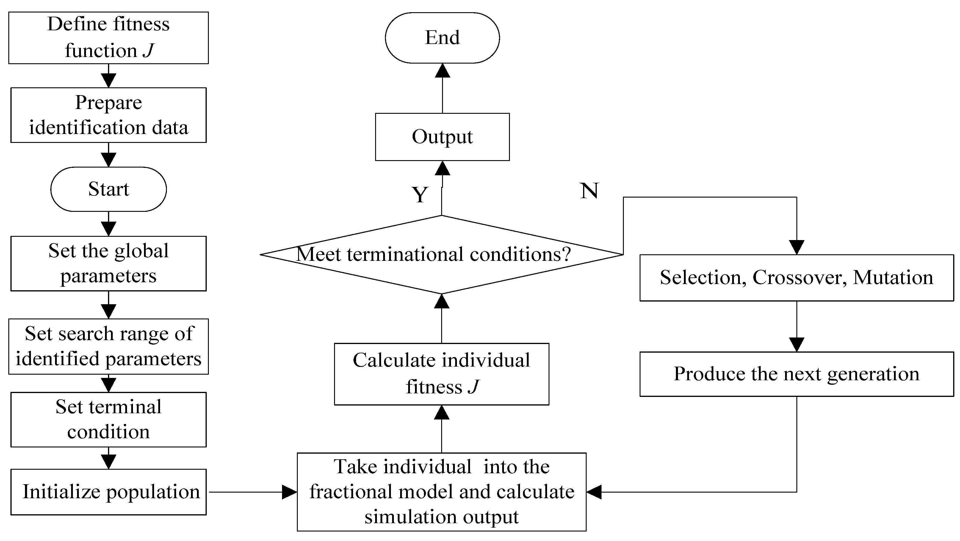
In this paper, the identification process is illustrated in Figure 1 based on the preceding analysis and basic operation process of GA. It can be seen from Figure 1 that the individual of population is composed of parameters to be identified. In the identification process, the binary encoding type and the initial population of 120 are selected. The optimization process will be stopped if one of three terminal conditions, which are 1,800 consecutive generations, 1,000 seconds runtime and 0.000001 fitness value, is satisfied.

Figure 1. Flow chart of fractional-order systems identification based on genetic algorithm.

Figure 1. Flow chart of fractional-order systems identification based on genetic algorithm.

4. Numerical Simulation and Results

4.1. Excitation Signals

The input signal is vital to system identification because it controls the output characteristics of the model [60,66]. Taken in this sense, it also determines the accuracy of identification results and whether the system is cognizable. Different systems need different optimal excitation signals to get more built-in features. Several input signals are selected to simulate the fractional-order system, including pseudo-random binary sequence (PRBS), sawtooth wave signal, sin-swept signal, and variable frequency signal (VFS). In this paper, PRBS and VFS are a periodic square wave signals; the frequency of sawtooth wave signal is 0.05 Hz; the sin-swept signal’s frequency increases from 0 to 200 Hz in one second linearly. The signals are generated by using signal functions in MATLAB. In addition, the amplitude of all the excitation signals is 1.00 and the length of data of each signal is 1,000. In engineering practice, the obtained data are contaminated by noise more or less because of the sensor precision and interference factors. To approach the actual situation, the output is joined by Gaussian white noise, and the input data have no noise.

Signal to Noise Ratio (SNR) is defined with the most commonly used method, as follows:

$$SNR=10{\log }_{10}\frac{YW}{NW}$$

(29)

where YW, NW express the powers of signal and noise respectively.

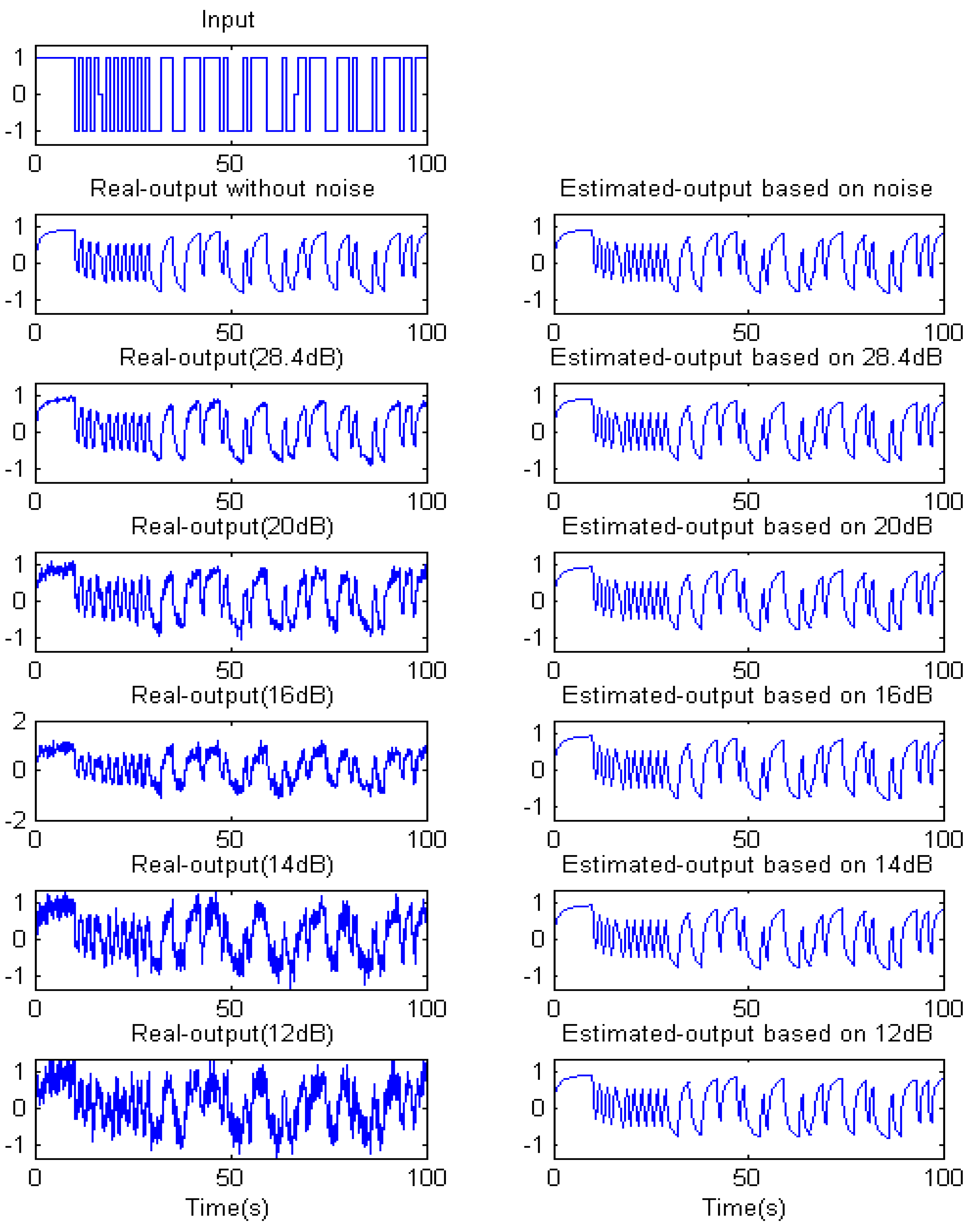
Figure 2. VFS excitation based on different noise levels of model (21).

Figure 2. VFS excitation based on different noise levels of model (21).

4.2. The Effect of Noise Level

It is well known that the noise often influences the accuracy of different identification methods. To estimate the sensitive extent of the proposed method, various noise levels of output signal is obtained by adding the Gaussian white noise, where the system input excitation is VFS without noise. The numerical simulations are carried out in the different noise level conditions. The external excitation and system response output with different SNR of model (21), and estimated output based on relevant final identification results are indicated in Figure 2 which includes output data with no noise, 28.4, 20, 16, 14 and 12 dB.

In order to reduce the stochastic error of each identification process, the mean and standard deviation of optimized parameters are adopted to evaluate the identification results. The identification result of each run is different. Therefore, in order to eliminate random error, the number of runs (five) was selected to calculate the statistical characteristics, such as the mean and standard deviation. The parameters listed in the paper are statistical values of multiple runs. For example, a, b, v are means of result of five times identifications; ${\sigma }_a$, ${\sigma }_b$, ${\sigma }_v$ are standard deviations of parameters. At the same time, the estimation index fit is introduced to evaluate the identification results fairly under different conditions. It can be viewed from Table 1 that, in case of on noise, the identified parameters are consistent with the true values and the fit is very close to 100% and the error could be ignored. In case of 20 dB noise level, the identification result presented in Table 1 shows that the means of identified parameters a, b, v are 0.976071, 0.988563 and 0.696444, respectively. In this condition, the maximum standard deviation is 2.33917 × 10⁻⁵ and the identification accuracy is 99.35%. While the SNR is 28.4 dB, the maximum standard deviation is 2.725825 × 10⁻⁵ and the parameter fit could reach to 99.58%. When the SNR is 16 dB, the fit is 99.18%. Even if the SNR is equal to 14 dB, the identification accuracy keeps 98.76% and its maximum standard deviation is 0.695666 × 10⁻⁵. However, when the noise continues to increase, the identification accuracy will become worse. The parameter fit is only 97.09% in case of 12 dB.

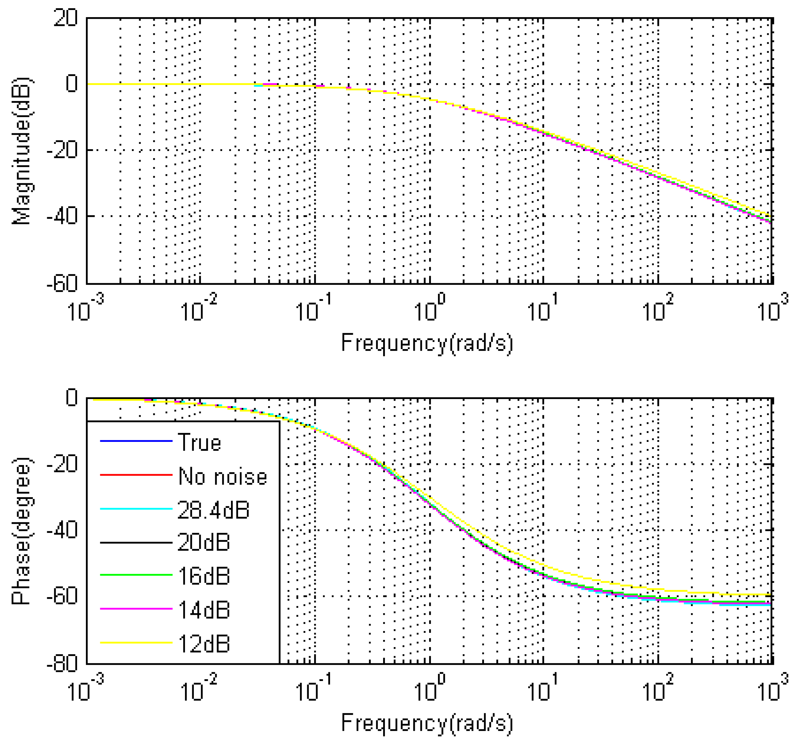
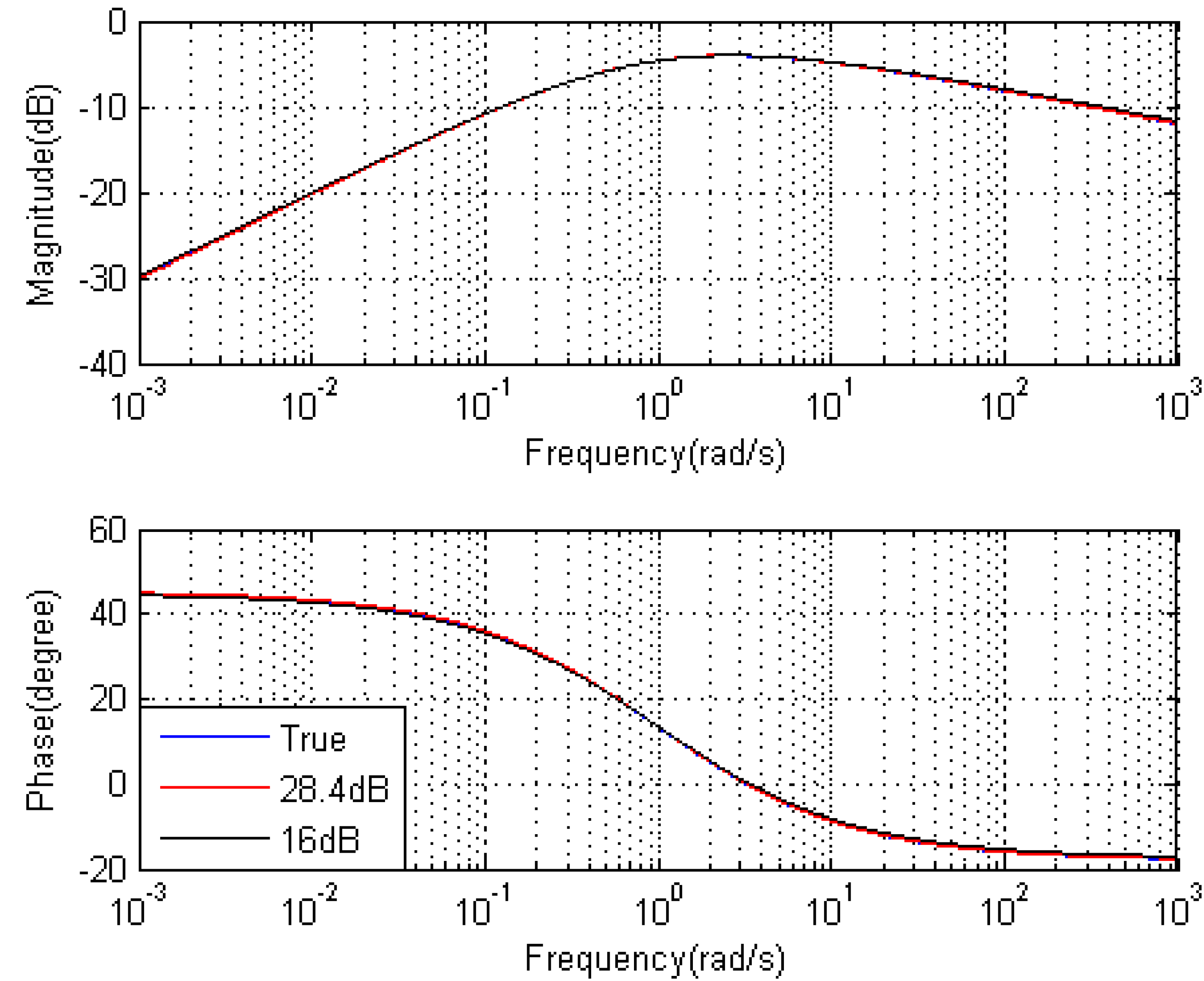
Figure 3. Identification results under different noise levels of model (21).

Figure 3. Identification results under different noise levels of model (21).

Figure 3 shows the Bode diagram of benchmark model (Equation (21), a = 1, b = 1, v = 0.7) and identified models under various noise levels, and Table 2 shows maximum errors of Magnitude and Phase between benchmark model and identified models in Figure 3. It can be seen from Figure 3 that estimated models have almost the same dynamic characteristics compared to the true one. In details, in case of on noise, the maximum errors of Magnitude and Phase are 5.8848 × 10⁻⁵ (dB) and 4.3329 × 10⁻⁴ (degree) orderly, and the error could be ignored. When the SNR is 28.4 dB, the maximum errors of Magnitude and Phase are merely −0.0205 and 0.0793 in turn. While the SNR is between 20 dB and 14 dB, the errors are closed to each other. The maximum errors of Magnitude and Phase are 0.1131, 0.3190 in case of 20 dB, 0.1376 and 0.3404 in case of 16 dB, 0.1269 and 0.3416 in case of 14 dB. However, when the SNR is 12 dB, the errors increase apparently, and they are 2.0961 dB and 3.3482 degrees. Therefore, from the above simulation and analysis results, it is obvious that the proposed method is insensitive to noise above 14 dB.

Table 1. Identification results based on different SNR of model (21).

Excitation	A	${\sigma }_a$ /10−5	b	${\sigma }_b$ /10−5	v	${\sigma }_v$ /10−5	fit
True	1		1		0.7
No noise	1.000034	0.960063	1.000018	0.869508	0.700011	0.508406	99.9997%
28.4 dB	1.006228	2.725825	0.999772	1.416844	0.701493	0.806250	99.58%
20 dB	0.976071	2.339170	0.988563	1.339580	0.696444	0.713023	99.35%
16 dB	0.972494	2.847766	0.988270	1.71262	0.696197	0.711188	99.18%
14 dB	0.958144	0.695666	0.972546	0.305697	0.696120	0.478331	98.76%
12 dB	1.007271	3.584513	1.016610	1.986676	0.667246	1.086456	97.09%

Table 1. Identification results based on different SNR of model (21).

Excitation	A	${\sigma }_a$ /10−5	b	${\sigma }_b$ /10−5	v	${\sigma }_v$ /10−5	fit
True	1		1		0.7
No noise	1.000034	0.960063	1.000018	0.869508	0.700011	0.508406	99.9997%
28.4 dB	1.006228	2.725825	0.999772	1.416844	0.701493	0.806250	99.58%
20 dB	0.976071	2.339170	0.988563	1.339580	0.696444	0.713023	99.35%
16 dB	0.972494	2.847766	0.988270	1.71262	0.696197	0.711188	99.18%
14 dB	0.958144	0.695666	0.972546	0.305697	0.696120	0.478331	98.76%
12 dB	1.007271	3.584513	1.016610	1.986676	0.667246	1.086456	97.09%

Table 2. Errors in frequency domain based on different SNR of model (21).

Error types	No noise	28.4 dB	20 dB	16 dB	14 dB	12 dB
Maximum error of Magnitude(dB)	5.8848 × 10−5	−0.0205	0.1131	0.1376	0.1269	2.0961
Maximum error of Phase(degree)	4.3329 × 10−4	0.0793	0.3190	0.3404	0.3416	3.3482

Table 2. Errors in frequency domain based on different SNR of model (21).

Error types	No noise	28.4 dB	20 dB	16 dB	14 dB	12 dB
Maximum error of Magnitude(dB)	5.8848 × 10−5	−0.0205	0.1131	0.1376	0.1269	2.0961
Maximum error of Phase(degree)	4.3329 × 10−4	0.0793	0.3190	0.3404	0.3416	3.3482

Figure 4. PRBS excitation output with SNR = 28.4dB of model (21)

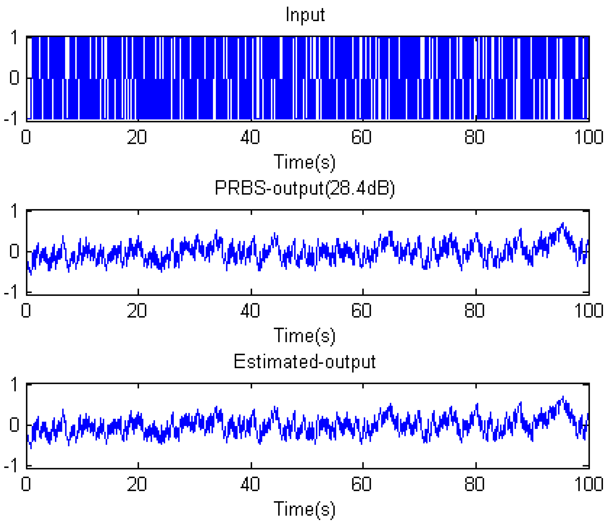
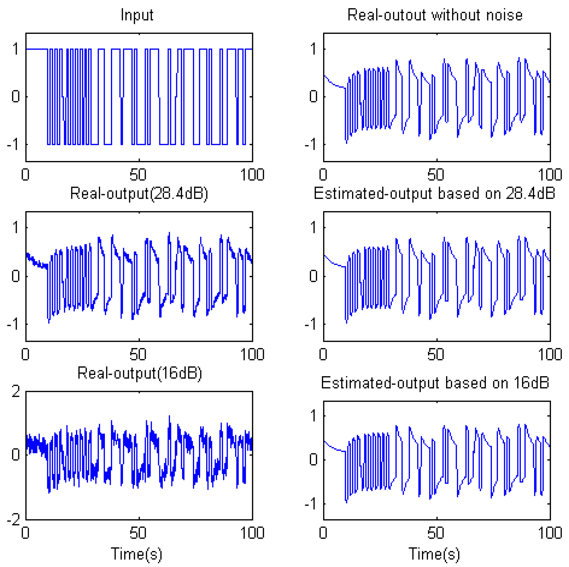
Figure 4. PRBS excitation output with SNR = 28.4dB of model (21)

4.3. The Effect of Excitation Signals

In the system identification, the external excitation is also an important factor to affect the identification accuracy. For the purpose of investigating the effect of excitation on identifying fractional-order system, this work designs various excitation signals, which include PRBS, VFS, sawtooth wave signal, and sin-swept signal. Meanwhile, the condition of numerical simulation is selected as system response with 28.4 dB noise level in order to keep the simulation conformable to reality. Different excitations and response outputs for the benchmark model (21), and estimated output based on relevant final identification results are indicated in Figure 2, Figure 4, Figure 5 and Figure 6. It is obvious that Figure 2 shows the system input and output under VFS excitation. Figure 4 describes the PRBS excitation. The system responses under sawtooth wave excitation and sin-swept signal excitation are exhibited in Figure 5 and Figure 6, respectively.

Figure 5. Sawtooth excitation output with SNR = 28.4 dB of model (21).

Figure 5. Sawtooth excitation output with SNR = 28.4 dB of model (21).

Figure 6. Sin-sweep excitation output with SNR = 28.4 dB of model (21).

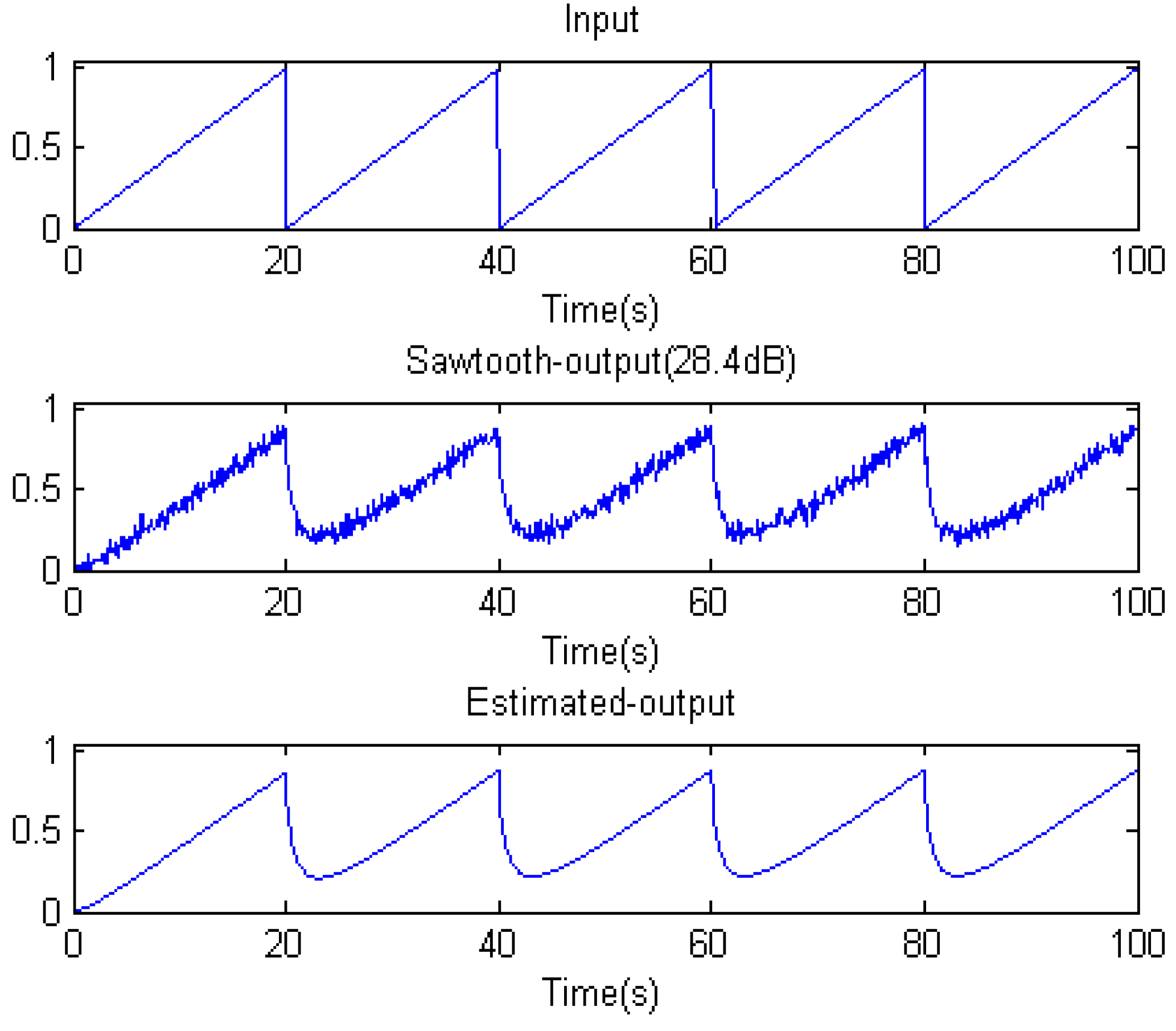
Figure 6. Sin-sweep excitation output with SNR = 28.4 dB of model (21).

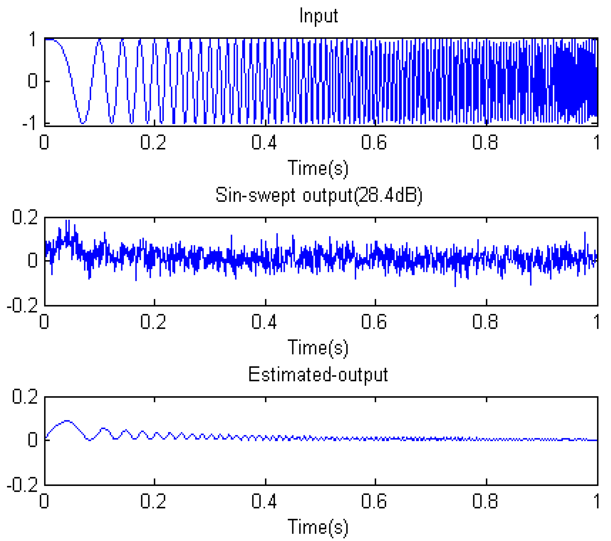
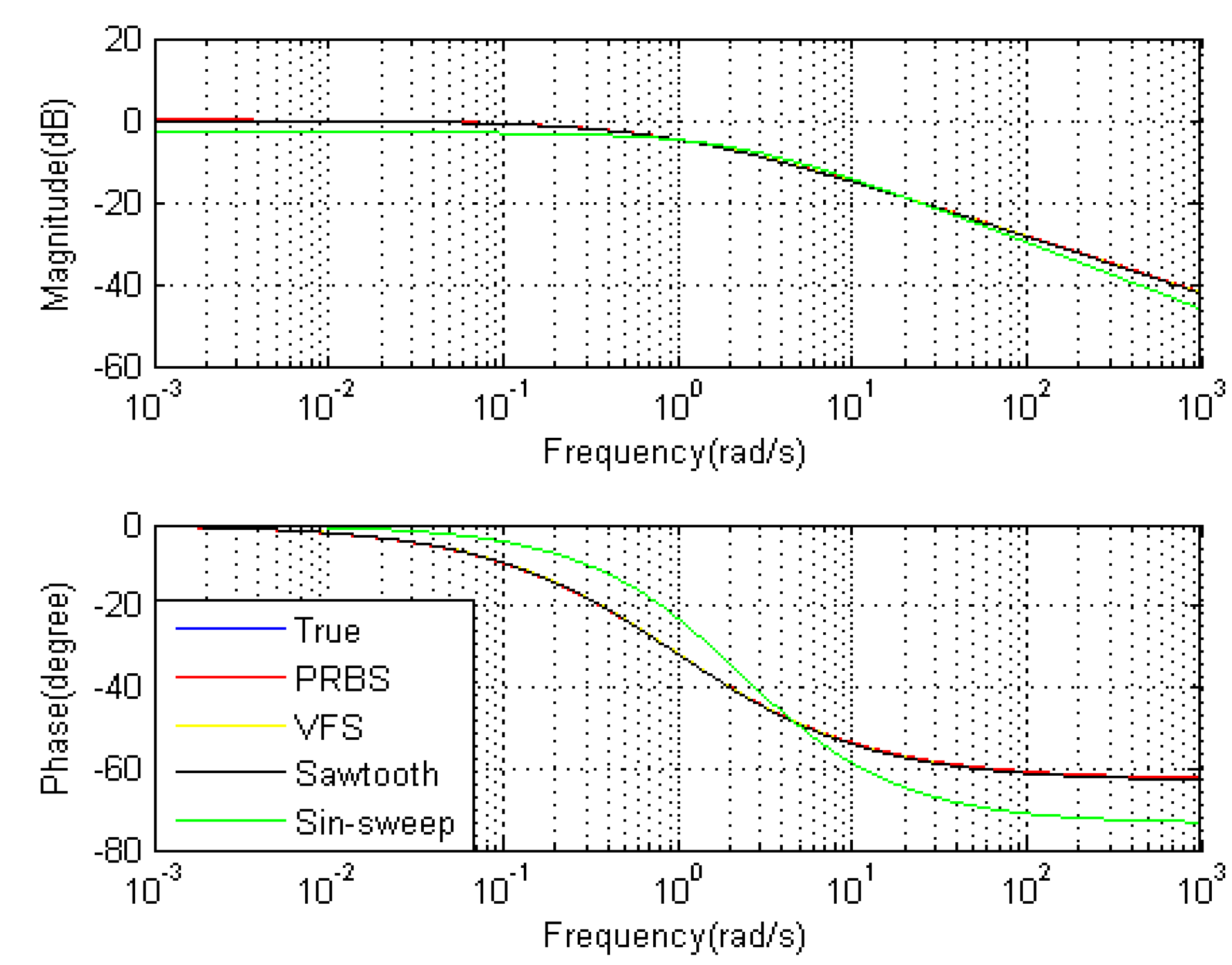
The identification results using the proposed method are listed in Table 3. It can be seen that the higher identification accuracy is obtained using PRBS and VFS excitation. The maximum accuracy reaches to 99.58% and its corresponding estimated parameters is 1.006228, 0.99538 and 0.701493. While adopting sawtooth wave excitation, the estimated values of a, b, v is 0.996426, 0992339 and 0.711274 and the fit is 98.67%. The worse results are obtained by using sin-swept signal excitation. In this case, the identification accuracy is 81.59% and its corresponding estimated parameters are 1.999999, 1.427971 and 0.817042. Figure 7 shows the Bode diagram of benchmark model and identified models under various excitations (SNR = 28.4 dB), and Table 4 shows the maximum errors of Magnitude and Phase between benchmark model and identified models in Figure 7. It can be seen from Figure 7 that estimated models under VFS and PRBS have almost the same dynamic characteristics compared to the true one. In addition, the maximum errors of Magnitude and Phase under VFS (−0.0205 dB, 0.0793 degree) are close to sawtooth wave excitation (0.0232 dB, 0.1052 degree), and are smaller than PRBS (0.1669 dB, 0.3146 degree). However, the errors are very big under sin-swept signal excitation, which are 0.9075 dB and 9.2118 degrees. Therefore, there is large difference between benchmark model and estimated model under sin-sweep excitation, which confirms the results in Table 3 and Table 4.

Figure 7. Identification results based on different excitations of model (21).

Figure 7. Identification results based on different excitations of model (21).

Table 3. Identification results based on different excitations of model (21).

Excitation	a	${\sigma }_a$ /10−5	b	${\sigma }_b$ /10−5	v	${\sigma }_v$ /10−5	fit
True	1		1		0.7
PRBS	0.985850	5.757508	0.995380	2.927489	0.696537	1.187264	99.51%
VFS	1.006228	2.725825	0.999772	1.416844	0.701493	0.806250	99.58%
Sawtooth	0.996426	1.329199	0.992339	1.266606	0.711274	0.222961	98.67%
Sin-sweep	1.999999	0.000415	1.427971	0.042450	0.817042	0.008724	81.59%

Table 3. Identification results based on different excitations of model (21).

Excitation	a	${\sigma }_a$ /10−5	b	${\sigma }_b$ /10−5	v	${\sigma }_v$ /10−5	fit
True	1		1		0.7
PRBS	0.985850	5.757508	0.995380	2.927489	0.696537	1.187264	99.51%
VFS	1.006228	2.725825	0.999772	1.416844	0.701493	0.806250	99.58%
Sawtooth	0.996426	1.329199	0.992339	1.266606	0.711274	0.222961	98.67%
Sin-sweep	1.999999	0.000415	1.427971	0.042450	0.817042	0.008724	81.59%

Table 4. Errors in frequency domain based on different excitations of model (21).

Error types	PRBS	VFS	Sawtooth	Sin-sweep
Maximum error of Magnitude(dB)	0.1669	−0.0205	0.0232	0.9075
Maximum error of Phase(degree)	0.3146	0.0793	0.1052	9.2118

Table 4. Errors in frequency domain based on different excitations of model (21).

Error types	PRBS	VFS	Sawtooth	Sin-sweep
Maximum error of Magnitude(dB)	0.1669	−0.0205	0.0232	0.9075
Maximum error of Phase(degree)	0.3146	0.0793	0.1052	9.2118

In this paper, identification results of the benchmark model (21) are more accurate based on square wave excitations such as PRBS and VFS excitation than sin-swept signal excitation. Therefore, it can be viewed that the external excitation plays a significant role in parameter identification of fractional-order systems. Because optimal excitation signal might arouse the most characters of the system, different systems need different optimal excitation signals to embody more features.

4.4. Identification of General Non-Commensurate Rate Fractional-Order System

In order to verify that the proposed method is effective for general model, the general non-commensurate rate fractional-order model (model (30)) is used as benchmark model for identification, as follows:

$$\frac{s^q}{s^v+1}$$

(30)

where q = 0.5, v = 0.7.

The external excitation (VFS) and system response output [model (30)] with different SNR which includes output data with 28.4 dB and 16 dB, and estimated output based on relevant final identification results are indicated in Figure 8.

Figure 8. VFS excitation with different noise levels of model (30).

Figure 8. VFS excitation with different noise levels of model (30).

The Bode diagrams of benchmark model and estimated models are shown in Figure 9. When the SNR is 28.4 dB, the fit is 99.62%, and maximum errors of Magnitude and Phase are 0.0337 dB and 0.3844 degree orderly. Estimated q is 0.503864 and v is 0.703319, and relevant standard deviations are 0.237492 × 10⁻⁵ and 0.319154 × 10⁻⁵. In case of 16 dB, estimated q is 0.497678 and v is 0.691340, and relevant standard deviations are 0.545049 × 10⁻⁵ and 0.716980 × 10⁻⁵. The fit is 99.26%, and maximum errors of Magnitude and Phase are 0.3775 dB and 0.6656 degree. The identified results prove that the proposed method is also suitable for general fractional-order systems.

Figure 9. Identification results of model (30).

Figure 9. Identification results of model (30).

5. Conclusions

This paper proposes an identification algorithm based on GA in the time domain with the weighted value of output error for fractional-order systems. The results verify that this algorithm can precisely identify the coefficients and fractional-order, even when the output mixed with noise. Taking the effective fitness function, GA can do the global search and solve the parameter identification issue for fractional-order systems. In addition, it is not enough to only use each parameter’s precision to evaluate the results on account of coupling among parameters. Taking errors between benchmark mode and estimated model both in the frequency domain and in the time domain as evaluation indices might be a good choice.

Excitation signal is of great importance for fractional-order systems identification; the best result might be found if the input is the optimal excitation signal of the system. However, it is very difficult to find the best signal, so it is important to select an input signal in accordance with specific conditions, which may base on antecedent analysis and experiences. What’s more, the results demonstrate that this method could identify the parameters of both commensurate rate and non-commensurate rate fractional-order systems from the data with noise. Exploring the application fractional-order systems identification to engineering practice is the further work in the future.

References

- Samko, S.G.; Kilbas, A.A.; Marichev, O.I. Fractional Integrals and Derivatives: Theory and applications; Gordon and Breach Science Publisher: New York, NY, USA, 1993. [Google Scholar]
- Oustaloup, A.; Levron, F.; Mathieu, B.; Nanot, F.M. Frequency-band complex noninteger differentiator: characterization and synthesis. IEEE Trans. Circuits and Systems I Fund. Theory Appl. 2000, 47, 25–40. [Google Scholar] [CrossRef]
- Oldham, K.B.; Spanier, J. The Fractional Calculus; Academic Press: New York, NY, USA, 1974. [Google Scholar]
- Miller, K.; Ross, B. An Introduction to the Fractional Calculus and Fractional Differential Equations; Wiley-Blackwell: New York, NY, USA, 1993. [Google Scholar]
- Vinagre, B.M.; Feliú, V.; Feliú, J.J. Frequency domain identification of a flexible structure with piezoelectric actuators using irrational transfer function models. In Proceedings of the 37th IEEE Conference on Decision and Control, Tampa, FL, USA, 16–18 December 1998; pp. 1278–1280.
- Lewandowski, R.; Chorazyczewski, B. Identification of the parameters of the Kelvin–Voigt and the Maxwell fractional models, used to modeling of viscoelastic dampers. Comput. Struct. 2010, 88, 1–17. [Google Scholar] [CrossRef]
- Dzielinski, A.; Sierociuk, D. Ultracapacitor modelling and control using discrete fractional order state-space model. Acta Montan. Slovaca 2008, 13, 136–145. [Google Scholar]
- Sabatier, J.; Aoun, M.; Oustaloup, A.; Grégoire, G.; Ragot, F.; Roy, P. Fractional system identification for lead acid battery state of charge estimation. Signal Process. 2006, 86, 2645–2657. [Google Scholar] [CrossRef]
- Suchorsky, M.K.; Rand, R.H. A pair of van der Pol oscillators coupled by fractional derivatives. Nonlinear Dynamics 2012, 69, 313–324. [Google Scholar] [CrossRef]
- Cao, J.Y.; Ma, C.B.; Xie, H.; Jiang, Z.D. Nonlinear dynamics of duffing system with fractional order damping. ASME J. Comput. Nonlinear Dyn. 2010, 5, 041012–041018. [Google Scholar] [CrossRef]
- Diethelm, K. A fractional calculus based model for the simulation of an outbreak of dengue fever. Nonlinear Dyn. 2013, 71, 613–619. [Google Scholar] [CrossRef]
- Yang, J.H.; Zhu, H. Vibrational resonance in Duffing systems with fractional-order damping. Chaos 2012, 22, 013112:1–013112:9. [Google Scholar] [CrossRef] [PubMed]
- Chen, W.; Zhang, X.D.; Cai, X. A study on modified Szabo’s wave equation modeling of frequency-dependent dissipation in ultrasonic medical imaging. Phys. Scripta 2009, T136, 014014. [Google Scholar] [CrossRef]
- Machado, J.T.; Galhano, A.S. Statistical fractional dynamics. J. Comput.Nonlinear Dyn. 2008, 3, 021201:1–021201:5. [Google Scholar] [CrossRef]
- Ubriaco, M.R. Entropies based on fractional calculus. Phys. Lett. A 2009, 373, 2516–2519. [Google Scholar] [CrossRef]
- Machado, J.A.T. Entropy analysis of integer and fractional dynamical systems. Nonlinear Dyn. 2010, 62, 371–378. [Google Scholar]
- Hoffmann, K.H.; Essex, C.; Schulzky, C. Fractional diffusion and entropy production. J. Non-Equilib. Thermodyn. 1998, 23, 166–175. [Google Scholar] [CrossRef]
- Essex, C.; Schulzky, C.; Franz, A.; Hoffmann, K.H. Tsallis and Rényi entropies in fractional diffusion and entropy production. Phys. Stat. Mech. Appl. 2000, 284, 299–308. [Google Scholar] [CrossRef]
- Prehl, J.; Essex, C.; Hoffmann, K.H. The super diffusion entropy production paradox in the space-fractional case for extended entropies. Phys. Stat. Mech. Appl. 2010, 389, 215–224. [Google Scholar] [CrossRef]
- Li, H.; Haldane, F.D.M. Entanglement spectrum as a generalization of entanglement entropy: identification of topological order in non-abelian fractional quantum hall effect states. Phys. Rev. Lett. 2008, 101, 010504. [Google Scholar] [CrossRef] [PubMed]
- Rossikhin, Y.A.; Shitikova, M.V. Application of fractional calculus for dynamic problems of solid mechanics: novel trends and recent results. J. Appl. Mech. Rev. 2010, 63, 1–52. [Google Scholar] [CrossRef]
- Baleanu, D.; Güvenç, Z.B.; Machado, J.A.T. New Trends in Nanotechnology and Fractional Calculus Applications; Springer-Verlag: New York, NY, USA, 2010. [Google Scholar]
- Sabatier, J.; Agrawal, O.P.; Machado, J.A.T. Advances in Fractional Calculus: Theoretical Developments and Applications in Physics and Engineering; Springer-Verlag: New York, NY, USA, 2007. [Google Scholar]
- Mathieu, B.; Melchior, P.; Oustaloup, A.; Ceyral, C. Fractional differentiation for edge detection. Signal Process. 2003, 83, 2421–2432. [Google Scholar] [CrossRef]
- Takayasu, H. Fractals in the Physical Sciences; St. Martin’s Press: New York, NY, USA, 1990. [Google Scholar]
- Fisher, Y. Fractal Image Compression: Theory and Application; Springer-Verlag: New York, NY, USA, 1995. [Google Scholar]
- Gabano, J.D.; Poinot, T.; Kanoun, H. Identification of a thermal system using continuous linear parameter-varying fractional modeling. Control Theory Appl. 2011, 5, 889–899. [Google Scholar] [CrossRef]
- Victor, S.; Melchior, P.; Nelson-Gruel, D.; Oustaloup, A. Flatness control for linear fractional MIMO systems: thermal application. In Proceedings of 3rd IFAC Workshop on Fractional Differentiation and Its Application, Ankara, Turkey, 5–7 November 2008; pp. 5–7.
- Ionescu, C.-M.; Hodrea, R.; de Keyser, R. Variable time-delay estimation for anesthesia control during intensive care. IEEE Trans. Biomed. Eng. 2011, 58, 363–369. [Google Scholar] [CrossRef] [PubMed]
- Sommacal, L.; Melchior, P.; Dossat, A.; Petit, J.; Cabelguen, J.-M.; Oustaloup, A.; Ijspeert, A.J. Improvement of the muscle fractional multimodel for low-rate stimulation. Biomed. Signal Process. Control 2007, 2, 226–233. [Google Scholar] [CrossRef]
- Sommacal, L.; Melchior, J.; Cabelguen, J.-M.; Oustaloup, A.; Ijspeert, A.J. Fractional Multi-Models of the Gastrocnemius Frog Muscle. J. Vib. Control 2008, 14, 1415–1430. [Google Scholar] [CrossRef]
- Oustaloup, A.; Sabatier, J.; Lanusse, P. From fractal robustness to the Crone control. Fract. Calc. Appl. Anal. 1999, 2, 1–30. [Google Scholar]
- Machado, J.A.T. Discrete-time fractional-order controllers. Fract. Calc. Appl. Anal. 2001, 4, 47–66. [Google Scholar]
- Monje, C.A.; Vinagre, B.M.; Feliu, V.; Chen, Y.Q. Tuning and auto-tuning of fractional order controllers for industry applications. Control Eng. Pract. 2008, 16, 798–812. [Google Scholar] [CrossRef]
- Chen, Y.Q.; Ahn, H.S.; Podlubny, I. Robust stability check of fractional order linear time invariant systems with interval uncertainties. Signal Process. 2006, 86, 2611–2618. [Google Scholar] [CrossRef]
- Zhao, M.C.; Wang, J.W. Outer synchronization between fractional-order complex networks: A non-fragile observer-based control scheme. Entropy 2013, 15, 1357–1374. [Google Scholar] [CrossRef]
- Barbosa, R.S.; Machado, J.A.T.; Silva, M.F. Time domain design of fractional differ integrators using least-squares. Signal Process. 2006, 86, 2567–2581. [Google Scholar] [CrossRef]
- Ortigueira, M.D.; Machado, J.A.T. Fractional signal processing and applications. Signal Process. 2003, 83, 2285–2286. [Google Scholar] [CrossRef]
- Melchior, P.; Orsoni, B.; Lavialle, O.; Poty, A.; Oustaloup, A. Consideration of obstacle danger level in path planning using A* and fast-marching optimisation: Comparative study. Signal Process. 2003, 83, 2387–2396. [Google Scholar] [CrossRef]
- Yousfi, N.; Melchior, P.; Rekik, C.; Derbel, N.; Oustaloup, A. Design of centralized CRONE controller combined with MIMO-QFT approach applied to non-square multivariable systems. Int. J. Comput. Appl. 2012, 45, 6–14. [Google Scholar]
- Yousfi, N.; Melchior, P.; Rekik, C.; Derbel, N.; Oustaloup, A. Path tracking design by fractional prefilter using a combined QFT/H∞ design for TDOF uncertain feedback systems. Nonlinear Dyn. 2013, 71, 701–712. [Google Scholar] [CrossRef]
- Ferreira, N.M.F.; Machado, J.A.T. Fractional-order hybrid control of robotic manipulators. In Proceedings of ICAR 2003, the 11th International Conference on Advanced Robotics, Coimbra, Portugal, 30 June–3 July 2003.
- Silva, M.F.; Machado, J.A.T.; Lopes, A.M. Fractional order control of a hexapod robot. Nonlinear Dyn. 2004, 38, 417–433. [Google Scholar] [CrossRef]
- Gaul, L.; Klein, P.; Kemple, S. Damping description involving fractional operators. Mech. Syst. Signal Process. 1991, 5, 81–88. [Google Scholar] [CrossRef]
- Cugnet, M.; Sabatier, J.; Laruelle, S.; Grugeon, S.; Sahut, B.; Oustaloup, A.; Tarascon, J.-M. Lead-acid battery fractional modeling associated to a model validation method for resistance and cranking capability estimation. IEEE Trans. Ind. Electron. 2010, 57, 909–917. [Google Scholar] [CrossRef]
- Sabatier, J.; Cugnet, M.; Laruelle, S.; Grugeon, S.; Sahut, B.; Oustaloup, A.; Tarascon, J.M. A fractional order model for lead-acid battery crankability estimation. Commun. Nonlinear Sci. Numer. Simul. 2010, 15, 1308–1317. [Google Scholar] [CrossRef]
- Baleanu, D.; Golmankhaneh, A.K.; Nigmatulli, R.; Golmankhaneh, A.K. Fractional Newtonian mechanics. Cent. Eur. J. Phys. 2010, 8, 120–125. [Google Scholar] [CrossRef]
- Herallah, M.A.E.; Baleanu, D. Fractional-order Euler–Lagrange equations and formulation of Hamiltonian equations. Nonlinear Dyn. 2009, 58, 385–391. [Google Scholar] [CrossRef]
- Sun, H.G.; Chen, W.; Chen, Y.Q. Variable-order fractional differential operators in anomalous diffusion modeling. Phys. Stat. Mech. Appl. 2009, 388, 4586–4592. [Google Scholar] [CrossRef]
- Chen, W.; Ye, L.J.; Sun, H.G. Fractional diffusion equations by the Kansa method. Comput. Math. Appl. 2010, 59, 1614–1620. [Google Scholar] [CrossRef]
- Li, C.P.; Peng, G.J. Chaos in Chen’s system with a fractional order. Chaos Soliton. Fract. 2007, 32, 443–450. [Google Scholar] [CrossRef]
- Yan, J.P.; Li, C.P. On chaos synchronization of fractional differential equations. Chaos Soliton. Fract. 2007, 32, 725–735. [Google Scholar] [CrossRef]
- Poinot, T.; Trigeassou, J.-C. Identification of fractional systems using an output-error technique. Nonlinear Dyn. 2004, 38, 133–154. [Google Scholar] [CrossRef]
- Cois, O.; Oustaloup, A.; Battaglia, E.; Battaglia, J.-L. Non integer model from modal decomposition for time domain system identification. In Proceedings of the 12th IFAC Symposium on System Identification, Santa Barbara, CA, USA, 21–23 June 2000; pp. 989–994.
- Lin, J.; Poinot, T.; Li, S.T.; Trigeassou, J.-C. Identification of non-integer-order systems in frequency domain. J. Control Theory Appl. 2008, 25, 517–520. [Google Scholar]
- Valério, D.; Costa, J.S.D. Identifying digital and fractional transfer functions from a frequency response. Int. J. Control 2011, 84, 445–457. [Google Scholar] [CrossRef]
- Poinot, T.; Trigeassou, J.-C. A method for modeling and simulation of fractional systems. Signal Process. 2003, 83, 2319–2333. [Google Scholar] [CrossRef]
- Hartley, T.T.; Lorenzo, C.F. Fractional-order system identification based on continuous order-distributions. Signal Process. 2003, 83, 2287–2300. [Google Scholar] [CrossRef]
- Nyikos, L.; Pajkossy, T. Fractal dimension and fractional power frequency-dependent impedance of blocking electrodes. Electrochim. Acta 1985, 30, 1533–1540. [Google Scholar] [CrossRef]
- Liu, D.H.; Cai, Y.W.; Su, Y.Z.; Yi, Y.X. Optimization method of parameter identification. In System Identification and Its Application, 1st ed.; Zhao, X.G., Yu, X.H., Eds.; National Defense Industry Press: Beijing, China, 2010; Volume 1, pp. 101–106. [Google Scholar]
- Goldberg, D.E.; Holland, J.H. Genetic Algorithms and Machine Learning. Mach. Learn. 1988, 3, 95–99. [Google Scholar] [CrossRef]
- Grefenstette, J.J. Optimization of control parameters for genetic algorithms. Syst. IEEE Trans. Man Cybern. 1986, 16, 122–128. [Google Scholar] [CrossRef]
- Harik, G.; Cantú-Paz, E.; Goldberg, D.E.; Miller, B.L. The gambler’s ruin problem, genetic algorithms, and the sizing of populations. In Proceedings of the IEEE International Conference on Evolutionary Computation, Ann Arbor, MI, USA, 13–16 April 1997; pp. 231–253.
- Miller, B.L.; Goldberg, D.E. Genetic algorithms, selection schemes, and the varying effects of noise. Evol. Comput. 1996, 4, 113–131. [Google Scholar] [CrossRef]
- Vale´rio, D.; Costa, J.S.D. Time-domain implementati on of fractional order controllers. IEEE Proc. Control Theory Appl. 2005, 152, 539–552. [Google Scholar] [CrossRef]
- Haber, R.; Keviczky, L. Nonlinear System Identification: Input-Output Modeling Approach; Springer-Verlag: New York, NY, USA, 1999. [Google Scholar]
© 2013 by the authors; licensee MDPI, Basel, Switzerland. This article is an open access article distributed under the terms and conditions of the Creative Commons Attribution license (http://creativecommons.org/licenses/by/3.0/).
Share and Cite
MDPI and ACS Style
Zhou, S.; Cao, J.; Chen, Y. Genetic Algorithm-Based Identification of Fractional-Order Systems. Entropy 2013, 15, 1624-1642. https://doi.org/10.3390/e15051624
AMA Style
Zhou S, Cao J, Chen Y. Genetic Algorithm-Based Identification of Fractional-Order Systems. Entropy. 2013; 15(5):1624-1642. https://doi.org/10.3390/e15051624
Chicago/Turabian StyleZhou, Shengxi, Junyi Cao, and Yangquan Chen. 2013. "Genetic Algorithm-Based Identification of Fractional-Order Systems" Entropy 15, no. 5: 1624-1642. https://doi.org/10.3390/e15051624