Bayesian and Quasi-Bayesian Estimators for Mutual Information from Discrete Data

Abstract

Mutual information (MI) quantifies the statistical dependency between a pair of random variables, and plays a central role in the analysis of engineering and biological systems. Estimation of MI is difficult due to its dependence on an entire joint distribution, which is difficult to estimate from samples. Here we discuss several regularized estimators for MI that employ priors based on the Dirichlet distribution. First, we discuss three “quasi-Bayesian” estimators that result from linear combinations of Bayesian estimates for conditional and marginal entropies. We show that these estimators are not in fact Bayesian, and do not arise from a well-defined posterior distribution and may in fact be negative. Second, we show that a fully Bayesian MI estimator proposed by Hutter (2002), which relies on a fixed Dirichlet prior, exhibits strong prior dependence and has large bias for small datasets. Third, we formulate a novel Bayesian estimator using a mixture-of-Dirichlets prior, with mixing weights designed to produce an approximately flat prior over MI. We examine the performance of these estimators with a variety of simulated datasets and show that, surprisingly, quasi-Bayesian estimators generally outperform our Bayesian estimator. We discuss outstanding challenges for MI estimation and suggest promising avenues for future research.

1. Introduction

Mutual information (MI) is a key statistic in science and engineering applications such as causality inference [1], dependency detection [2], and estimation of graphical models [3]. Mutual information has the theoretical virtue of being invariant to the particular coding of variables. As a result, it has been widely used to quantify the information carried by neural spike trains, where the coding is typically not known a priori [4].

One approach to mutual information estimation is to simplify the problem using a breakdown of MI into marginal and conditional entropies (see Equation (2)). These entropies can be estimated separately and then combined to yield a consistent estimator for MI. As we will show, three different breakdowns yield three distinct estimators for MI. We will call these estimates “quasi-Bayesian” when they arise from combinations of Bayesian entropy estimates.

A vast literature has examined the estimation of Shannon’s entropy, which is an important problem in its own right [5,6,7,8,9,10,11,12,13,14,15,16]. Among the most popular methods is a Bayes Least Squares (BLS) estimator known as Nemenman–Shafee–Bialek (NSB) estimator [17]. This estimator employs a mixture-of-Dirichlets prior over the space of discrete distributions, with mixing weights selected to achieve an approximately flat prior over entropy. The BLS estimate corresponds to the mean of the posterior over entropy.

A second, “fully Bayesian” approach to MI estimation is to formulate a prior over the joint probability distribution in question and compute the mean of the induced posterior distribution over MI. Hutter showed that the BLS estimate (i.e., posterior mean) for MI under a Dirichlet prior has an analytic form [18]. To our knowledge, this is the only fully Bayesian MI estimator proposed thus far, and its performance has never been evaluated empirically (but see [19]).

We begin, in Section 2, with a brief introduction to entropy and mutual information. In Section 3, we review Bayesian entropy estimation, focusing on the NSB estimator and the intuition underlying the construction of its prior. In Section 4, we show that the MI estimate resulting from a linear combination of BLS entropy estimates is not itself Bayesian. In Section 5, we examine the MI estimator introduced by Hutter [18] and show that it induces a narrow prior distribution over MI, leading to large bias and excessively narrow credible intervals for small datasets. We formulate a novel Bayesian MI estimator using a mixture-of-Dirichlets prior, designed to have a maximally uninformative prior over MI. Finally, in Section 6, we compare the performance of Bayesian and quasi-Bayesian estimators on a variety of simulated datasets.

2. Entropy and Mutual Information

Consider data samples ${\left(x_i,y_i\right)}_{i=1}^N$ drawn iid from π, a discrete joint distribution for random variables X and Y. Assume that these variables take values on finite alphabets $\{1,\dots ,K_x\}$ and $\{1,\dots ,K_y\}$, respectively, and define ${\pi }_{ij}=p(X=i,Y=j)$. Note that π can be represented as a $K_x\times K_y$ matrix, and that ${\sum }_i{\sum }_j{\pi }_{ij}=1$. The entropy of the joint distribution is given by

$$H(\pi )=-\sum _{i=1}^{K_x}\sum _{j=1}^{K_y}{\pi }_{ij}log{\pi }_{ij}$$

(1)

where log denotes the logarithm base 2 (We denote the natural logarithm by ln; that is, $logx=\frac{lnx}{ln2}$). The mutual information between X and Y is also a function of π. It can be written in terms of entropies in three different but equivalent forms:

$$\begin{array}{}\mathrm{(2)}& \hfill I(\pi )& =& H({\pi }_y)+H({\pi }_x)-H(\pi )\hfill \mathrm{(3)}& & =& H({\pi }_x)-\sum _{j=1}^{K_y}{\pi }_{y_j}H({\pi }_{x|y_j})\hfill \mathrm{(4)}& & =& H({\pi }_y)-\sum _{i=1}^{K_x}{\pi }_{x_i}H({\pi }_{y|x_i})\hfill \end{array}$$

where we use ${\pi }_x$ and ${\pi }_y$ to denote the marginal distributions of X and Y, respectively, ${\pi }_{x|y_j}=p(X|Y=j)$ and ${\pi }_{y|x_i}=p(Y|X=i)$ to denote the conditionals, and ${\pi }_{x_i}=p(X=i)$ and ${\pi }_{y_j}=p(Y=j)$ to denote the elements of the marginals.

The simplest approach for estimating joint entropy $H(X,Y)$ and mutual information $I(X,Y)$ is to directly estimate the joint distribution π from counts $n_{ij}={\sum }_{n=1}^N{\mathbf{1}}_{\left\{(x_n,y_n)=(i,j)\right\}}$. These counts yield the empirical joint distribution $\widehat{\pi }$, where ${\widehat{\pi }}_{ij}=n_{ij}/N$. Plugging $\widehat{\pi }$ into Equations (1) and (2) yields the so-called “plugin” estimators for entropy and mutual information: ${\widehat{H}}_{\text{plugin}}=H(\widehat{\pi })$ and ${\widehat{I}}_{\text{plugin}}=I(\widehat{\pi })$, respectively. To compute ${\widehat{I}}_{\text{plugin}}$ we estimate the marginal distributions ${\pi }_x$ and ${\pi }_y$ via the marginal counts $n_{y_j}={\sum }_{i=1}^{K_x}{n}_{ij}$ and $n_{x_i}={\sum }_{j=1}^{K_y}{n}_{ij}$. The plugin estimators are the maximum-likelihood estimators under multinomial likelihood. Although these estimators are straightforward to compute, they unfortunately exhibit substantial bias unless π is well-sampled: ${\widehat{H}}_{\text{plugin}}$ exhibits negative bias and, as a consequence, ${\widehat{I}}_{\text{plugin}}$ exhibits positive bias [8,20]. There are many proposed methods for removing these biases, which generally attempt to compensate for the excessive “roughness” of $\widehat{\pi }$ that arises from undersampling. Here, we focus on Bayesian methods, which regularize using an explicit prior distributions over π.

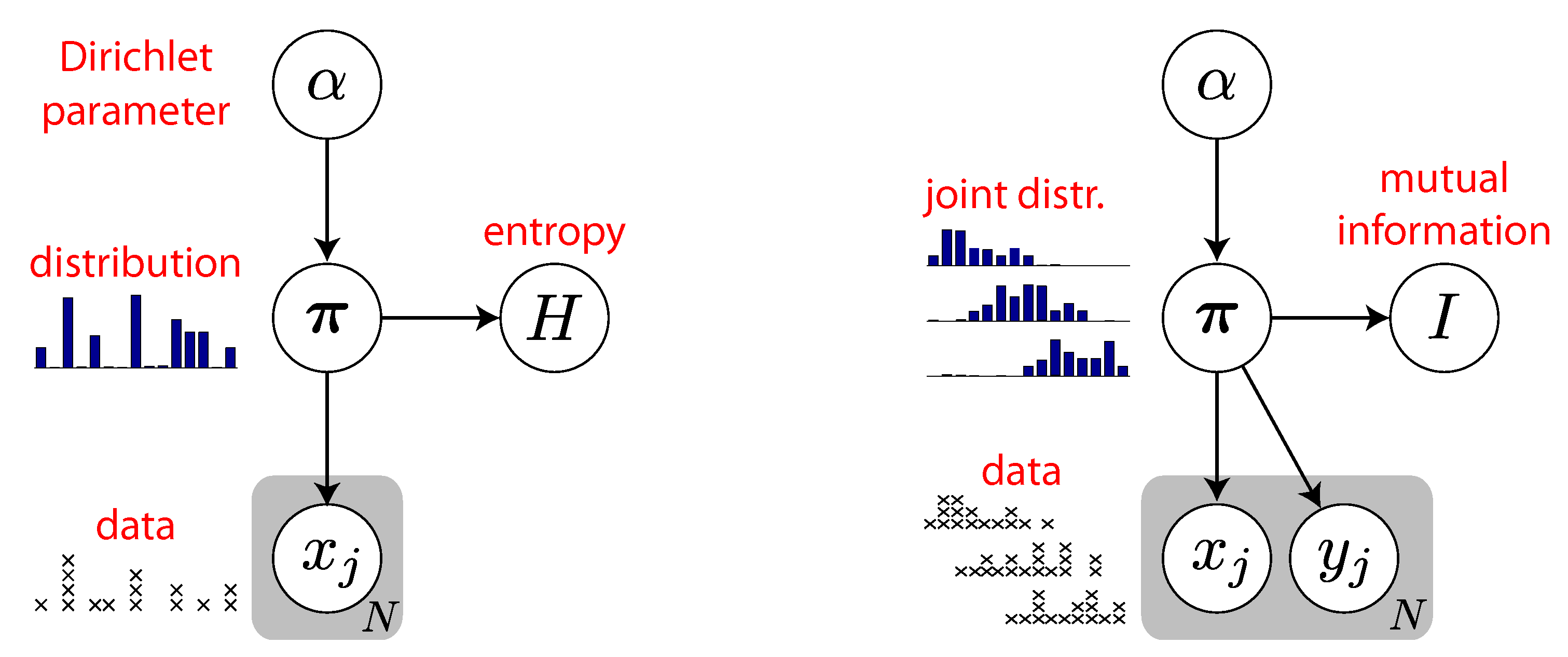
3. Bayesian Entropy Estimation

We begin by reviewing the NSB estimator [17], a Bayes least squares (BLS) estimator for H under the generative model depicted in Figure 1. The Bayesian approach to entropy estimation involves formulating a prior over distributions π, and then turning the crank of Bayesian inference to infer H using the posterior over H induced by the posterior over π. The starting point for this approach is the symmetric Dirichlet prior with parameter α over a discrete distribution π:

$$p(\pi |\alpha )=\text{Dir}(\alpha )\triangleq \text{Dir}(\alpha ,\alpha ,\dots ,\alpha )=\frac{\Gamma (K\alpha )}{\Gamma {(\alpha )}^K}\prod _{i=1}^K{\pi }_i^{\alpha -1}(Dirichlet prior)$$

(5)

where ${\pi }_i$ (the ith element of the vector π) gives the probability that a data point x falls in the ith bin, K denotes the number of bins in the distribution, and ${\sum }_{i=1}^K{\pi }_i=1$. The Dirichlet concentration parameter $\alpha >0$ controls the concentration or “roughness” of the prior, with small α giving spiky distributions (most probability mass concentrated in a few bins) and large α giving more uniform distributions.

Figure 1. Graphical models for entropy and mutual information of discrete data. Arrows indicate conditional dependencies between variables and gray “plates” indicate N independent draws of random variables. Left: Graphical model for entropy estimation [16,17]. The probability distribution over all variables factorizes as $p(\alpha ,\pi ,\mathbf{x},H)=p(\alpha )p(\pi |\alpha )p(\mathbf{x}|\pi )p(H|\pi )$, where $p(H|\pi )$ is simply a delta measure on $H(\pi )$. The hyper-prior $p(\alpha )$ specifies a set of “mixing weights” for Dirichlet distributions $p(\pi |\alpha )=\text{Dir}(\alpha )$ over discrete distributions π. Data $\mathbf{x}=\left\{x_j\right\}$ are drawn from the discrete distribution π. Bayesian inference for H entails integrating out α and π to obtain the posterior $p(H|\mathbf{x})$. Right: Graphical model for mutual information estimation, in which π is now a joint distribution that produces paired samples $\left\{(x_j,y_j)\right\}$. The mutual information I is a deterministic function of the joint distribution π. The Bayesian estimate comes from the posterior $p(I|\mathbf{x})$, which requires integrating out π and α.

Figure 1. Graphical models for entropy and mutual information of discrete data. Arrows indicate conditional dependencies between variables and gray “plates” indicate N independent draws of random variables. Left: Graphical model for entropy estimation [16,17]. The probability distribution over all variables factorizes as $p(\alpha ,\pi ,\mathbf{x},H)=p(\alpha )p(\pi |\alpha )p(\mathbf{x}|\pi )p(H|\pi )$, where $p(H|\pi )$ is simply a delta measure on $H(\pi )$. The hyper-prior $p(\alpha )$ specifies a set of “mixing weights” for Dirichlet distributions $p(\pi |\alpha )=\text{Dir}(\alpha )$ over discrete distributions π. Data $\mathbf{x}=\left\{x_j\right\}$ are drawn from the discrete distribution π. Bayesian inference for H entails integrating out α and π to obtain the posterior $p(H|\mathbf{x})$. Right: Graphical model for mutual information estimation, in which π is now a joint distribution that produces paired samples $\left\{(x_j,y_j)\right\}$. The mutual information I is a deterministic function of the joint distribution π. The Bayesian estimate comes from the posterior $p(I|\mathbf{x})$, which requires integrating out π and α.

The likelihood (bottom arrow in Figure 1, left) is the conditional probability of the data x given π:

$$p(\mathbf{x}|\pi )=\frac{N!}{{\prod }_i{n}_i!}\prod _{i=1}^K{\pi }_i^{n_i}(multinomial likelihood)$$

(6)

where $n_i$ is the number of samples in x falling in the ith bin, and N is the total number of samples. Because Dirichlet is conjugate to multinomial, the posterior over π given α and x takes the form of a Dirichlet distribution:

$$p(\pi |\mathbf{x},\alpha )=\text{Dir}(\alpha +n_1,\dots ,\alpha +n_K)=\Gamma (K\alpha +N)\prod _{i=1}^K\frac{{\pi }_i^{n_i+\alpha -1}}{\Gamma (\alpha +n_i)}(Dirichlet posterior)$$

(7)

From this expression, the posterior mean of H can be computed analytically [17,21]:

$$\begin{array}{cc}\mathrm{(8)}& \hfill {\widehat{H}}_{Dir}(\alpha )=\mathbb{E}\left[H\right|\mathbf{x},\alpha ]& =\int H(\pi )p(\pi |\mathbf{x},\alpha )d\pi \hfill & =\frac{1}{ln2}\left[{\psi }_0(N+K\alpha +1)-\sum _i\frac{(n_i+\alpha )}{(N+\alpha K)}{\psi }_0(n_i+\alpha +1)\right]\hfill \end{array}$$

where ${\psi }_n$ is the polygamma function of n-th order (${\psi }_0$ is the digamma function). For each α, ${\widehat{H}}_{Dir}(\alpha )$ is the posterior mean of a Bayesian entropy estimator with a $\text{Dir}(\alpha )$ prior. Nemenman and colleagues [17] observed that, unless $N\gg K$, the estimate ${\widehat{H}}_{Dir}$ is strongly determined by the Dirichlet parameter α. They suggested using a hyper-prior $p(\alpha )$ over the Dirichlet parameter, resulting in a mixture-of-Dirichlets distributions prior:

$$p(\pi )=\int p(\pi |\alpha )p(\alpha )d\alpha (prior)$$

(9)

The NSB estimator is the posterior mean of $p(H|\mathbf{x})$ under this prior, which can in practice be computed by numerical integration over α with appropriate weighting of ${\widehat{H}}_{Dir}(\alpha )$:

$${\widehat{H}}_{NSB}=\mathbb{E}\left[H\right|\mathbf{x}]=\int \int H(\pi )p(\pi |\mathbf{x},\alpha )p(\alpha |\mathbf{x})d\pi d\alpha =\int {\widehat{H}}_{Dir}(\alpha )p(\alpha |\mathbf{x})d\alpha$$

(10)

By Bayes’ rule, we have $p(\alpha |\mathbf{x})\propto p(\mathbf{x}|\alpha )p(\alpha )$, where $p(\mathbf{x}|\alpha )$, the marginal probability of x given α, takes the form of a Polya distribution [22]:

$$p(\mathbf{x}|\alpha )=\int p(\mathbf{x}|\pi )p(\pi |\alpha )d\pi =\frac{(N!)\Gamma (K\alpha )}{\Gamma {(\alpha )}^K\Gamma (N+K\alpha )}\prod _{i=1}^K\frac{\Gamma (n_i+\alpha )}{n_i!}$$

(11)

To obtain an uninformative prior on the entropy, [17] proposed the (hyper-)prior

$$p_{\text{NSB}}(\alpha )\propto \frac{\mathrm{d}\mathbb{E}\left[H\right|\alpha ]}{\mathrm{d}\alpha }=\frac{1}{ln2}\left[K{\psi }_1(K\alpha +1)-{\psi }_1(\alpha +1)\right],$$

(12)

the derivative with respect to α of the prior mean of the entropy (i.e., before any data have been observed, which depends only on the number of bins K). This prior may be computed numerically (from Equation (12)) using a fine discretization of α. In practice, we find that a prior representation in terms of log α is more tractable since the derivative is extremely steep near zero; the prior on log α has a more approximately smooth bell shape (see Figure 2A).

The NSB prior would provide a uniform prior over entropy if the distribution p(H|α) were a delta function. In practice, the implied prior on H is not entirely flat, especially for small K (see Figure 2B).

Figure 2. NSB priors used for entropy estimation, for three different values of alphabet size K. (A) The NSB hyper-prior on the Dirichlet parameter α on a log scale (Equation (12)). (B) Prior distributions on H implied by each of the three NSB hyper-priors in (A). Ideally, the implied prior over entropy should be as close to uniform as possible.

Figure 2. NSB priors used for entropy estimation, for three different values of alphabet size K. (A) The NSB hyper-prior on the Dirichlet parameter α on a log scale (Equation (12)). (B) Prior distributions on H implied by each of the three NSB hyper-priors in (A). Ideally, the implied prior over entropy should be as close to uniform as possible.

3.1. Quantifying Uncertainty

Credible intervals (Bayesian confidence intervals) can be obtained from the posterior variance of H|x, which can be computed by numerically integrating the variance of entropy across α. The raw second moment of the posterior is, from [16,21]:

$$\begin{array}{c}\hfill \mathbb{E}\left[H^2\right|\mathbf{x},\alpha ]=\frac{1}{ln{(2)}^2}\sum _i\frac{(n_i^{\prime }+1)(n_i^{\prime })}{\nu (\nu +1)}\left[{({\psi }_0(n_i^{\prime }+2)-{\psi }_0(\nu +2))}^2+{\psi }_1(n_i^{\prime }+2)-{\psi }_1(\nu +2)\right]\\ \mathrm{(13)}& \hfill +\frac{1}{ln{(2)}^2}\sum _{i\ne k}\frac{n_i^{\prime }{n}_k^{\prime }}{\nu (\nu +1)}\left[({\psi }_0(n_k^{\prime }+1)-{\psi }_0(\nu +2))({\psi }_0(n_i^{\prime }+1)-{\psi }_0(\nu +2))-{\psi }_1(\nu +2)\right]\end{array}$$

where $n_i^{\prime }=n_i+\alpha$ and $\nu =N+\alpha K$. As above, this expression can be integrated numerically with respect to $p(\alpha |\mathbf{x})$ to obtain the second moment of the NSB estimate:

$$\mathbb{E}\left[H^2\right|\mathbf{x}]=\int \mathbb{E}\left[H^2\right|\mathbf{x},\alpha ]p(\alpha |\mathbf{x})d\alpha$$

(14)

giving posterior variance $\mathbb{V}\text{ar}(H|\mathbf{x})=\mathbb{E}\left[H^2\right|\mathbf{x}]-E{\left[H\right|\mathbf{x}]}^2$.

3.2. Efficient Computation

Computation of the posterior mean and variance under the NSB prior can be carried out more efficiently using a representation in terms of multiplicities, also known as the empirical histogram distribution function [8], which is the number of bins in the empirical distribution with each count. Let $z_n=\left|\{i;n_i=n\}\right|$ denote the number of histogram bins with exactly n samples. This gives the compressed statistic $\mathbf{z}={[z_0,z_1,\cdots ,z_{n_{\text{max}}}]}^T$, where $n_{\text{max}}$ is the largest number of samples in a single histogram bin. Note that the dot product $[0,1,\dots ,n_{\text{max}}]\mathbf{z}=N$, is the total number of samples in the dataset.

The advantage of this representation is that we only need to compute sums and products involving the number of bins with distinct counts (at most $n_{\text{max}}$), rather than the total number of bins K. We can use this representation for any expression not explicitly involving π, such as the marginal probability of x given α (Equation (11)),

$$p(\mathbf{x}|\alpha )=\frac{(N!)\Gamma (K\alpha )}{\Gamma {(\alpha )}^K\Gamma (N+K\alpha )}\prod _{n=0}^{n_{\text{max}}}{\left(\frac{\Gamma (n+\alpha )}{n!}\right)}^{z_n}$$

(15)

and the posterior mean of H given α (Equation (8)), given by

$${\widehat{H}}_{\text{Dir}}=\mathbb{E}\left[H\right|\mathbf{x},\alpha ]=\frac{1}{ln2}\left[{\psi }_0(N+\alpha K+1)-\sum _{n=0}^{n_{\text{max}}}\frac{z_n(n+\alpha )}{N+\alpha K}{\psi }_0(n+\alpha +1)\right]$$

(16)

which are the two ingredients we need to numerically compute ${\widehat{H}}_{\text{NSB}}$ (Equation (10)).

4. Quasi-Bayesian Estimation of MI

The problem of estimating mutual information between a pair of random variables is distinct from the problem of estimating entropy. However, it presents many of the same challenges, since the maximum likelihood estimators for both entropy and mutual information are biased [8]. One way to regularize an estimate for MI is to use Bayesian estimates for the entropies appearing in the decompositions of MI (given in Equations (2), (3), and (4)) and combine them appropriately. We refer to the resulting estimates as “quasi-Bayesian”, since (as we will show below) they do not arise from any well-defined posterior distribution.

Consider three different quasi-Bayesian estimators for mutual information, which result from distinct combinations of NSB entropy estimates:

$$\begin{array}{}\mathrm{(17)}& \hfill {\widehat{I}}_{\text{NSB1}}(\pi )& ={\widehat{H}}_{\text{NSB}}({\pi }_x)+{\widehat{H}}_{\text{NSB}}({\pi }_y)-{\widehat{H}}_{\text{NSB}}(\pi )\hfill \mathrm{(18)}& \hfill {\widehat{I}}_{\text{NSB2}}(\pi )& ={\widehat{H}}_{\text{NSB}}({\pi }_x)-\sum _{j=1}^{K_y}{\widehat{\pi }}_{y_i}{\widehat{H}}_{\text{NSB}}({\pi }_{x|y_j})\hfill \mathrm{(19)}& \hfill {\widehat{I}}_{\text{NSB3}}(\pi )& ={\widehat{H}}_{\text{NSB}}({\pi }_y)-\sum _{i=1}^{K_x}{\widehat{\pi }}_{x_i}{\widehat{H}}_{\text{NSB}}({\pi }_{y|x_i})\hfill \end{array}$$

The first of these (${\widehat{I}}_{\text{NSB1}}$) combines estimates of the marginal entropies of ${\pi }_x$ and ${\pi }_y$ and the full joint distribution π, while the other two (${\widehat{I}}_{\text{NSB2}}$ and ${\widehat{I}}_{\text{NSB3}}$) rely on weighted combinations of estimates of marginal and conditional entropies. Although the three algebraic breakdowns of MI are mathematically identical, the three quasi-Bayesian estimators defined above are in general different, and they can exhibit markedly different performance in practice.

Studies in the nervous system often use ${\widehat{I}}_{\text{NSB3}}$ to estimate the MI between sensory stimuli and neural responses, an estimator commonly known as the “direct method” [7], motivated by the fact that the marginal distribution over stimuli ${\pi }_x$ is either pre-specified by the experimenter or well-estimated from the data [4,23]. In these experiments, the number of stimuli $K_x$ is typically much smaller than the number of possible neural responses $K_y$, which makes this approach reasonable. However, we show that ${\widehat{I}}_{\text{NSB3}}$ does not achieve the best empirical performance of the three quasi-Bayesian estimators, at least for the simulated examples we consider below.

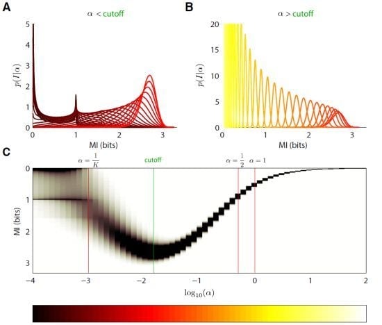
4.1. Bayesian Entropy Estimates do not Give Bayesian MI Estimates

Bayesian estimators require a well-defined posterior distribution. A linear combination of Bayesian estimators does not produce a Bayesian estimator unless the estimators can be combined in a manner consistent with a single underlying posterior. In the case of entropy estimation, the NSB prior depends on the number of bins K. Consequently, the priors over the marginal distributions ${\pi }_x$ and ${\pi }_y$, which have $K_x$ and $K_y$ bins, respectively, are not equal to the priors implied by marginalizing the NSB prior over the joint distribution π, which has $K_x{K}_y$ bins. This means that ${\widehat{H}}_{\text{NSB}}({\pi }_x)$, ${\widehat{H}}_{\text{NSB}}({\pi }_y)$, and ${\widehat{H}}_{\text{NSB}}(\pi )$ are Bayesian estimators under inconsistent prior distributions over the pieces of π. Combining them to form ${\widehat{I}}_{\text{NSB1}}$ (Equation (17)) results in an estimate that is not Bayesian, as there is no well-defined posterior over I given the data.

The same inconsistency arises for ${\widehat{I}}_{\text{NSB2}}$ and ${\widehat{I}}_{\text{NSB3}}$, which combine Bayesian entropy estimates under incompatible priors over the conditionals and marginals of the joint distribution. To wit, ${\widehat{I}}_{\text{NSB2}}$ assumes the conditionals ${\pi }_{x|y_i}$ and the marginal ${\pi }_x$ are a priori independent and identically distributed (i.e., with uniform entropy on $[0,log{K}_x]$ as specified by the NSB prior). This is incompatible with the fact that the marginal is a convex combination of the conditionals, and therefore entirely dependent on the distribution of the conditionals. We state the general observation as follows:

Proposition 1. 

The estimators ${\widehat{I}}_{\text{NSB1}}$, ${\widehat{I}}_{\text{NSB2}}$, or ${\widehat{I}}_{\text{NSB3}}$ are not Bayes least squares estimators for mutual information.

To establish this proposition, it suffices to show that there is a dataset for which the quasi-Bayesian estimates are negative. Since MI can never be negative, the posterior cannot have negative support, and the Bayesian least squares estimate must therefore be non-negative. It is easy to find datasets with small numbers of observations for which the quasi-Bayesian estimates are negative. Consider a dataset from a joint distribution on 3 × 3 bins, with counts given by $\left[\begin{array}{ccc}0& 1& 0\\ 1& 10& 1\\ 0& 1& 0\end{array}\right]$. Although the plugin estimate for MI is positive (0.02 bits), all three quasi-Bayesian estimates are negative: ${\widehat{I}}_{\text{NSB1}}=-0.07$ bits, and ${\widehat{I}}_{\text{NSB2}}={\widehat{I}}_{\text{NSB3}}=-0.05$ bits. Even more negative values may be obtained when this 3 × 3 table is embedded in a larger table of zeros. This discrepancy motivates the development of fully Bayesian estimators for MI under a single, consistent prior over joint distributions, a topic we address in the next section.

5. Fully Bayesian Estimation of MI

A Bayes least squares estimate for MI is given by the mean of a well-defined posterior distribution over MI. The first such estimator, proposed originally by [18], employs a Dirichlet prior over the joint distribution π. The second, which we introduce here, employs a mixture-of-Dirichlets prior, which is conceptually similar to the NSB prior in attempting to achieve a maximally flat prior distribution over the quantity of interest.

5.1. Dirichlet Prior

Consider a Dirichlet prior with identical concentration parameters α over the joint distribution of $X\times Y$, defined by a probability table of size $K_x\times K_y$ (see Figure 1). This prior treats the joint distribution π as a simple distribution on $K=K_x{K}_y$ bins, ignoring any joint structure. Nevertheless, the properties of the Dirichlet distribution again prove convenient for computation. While table π is distributed just as a probability vector in Equation (2), by the aggregation property of the Dirichlet distribution, the marginals of π are also Dirichlet distributed:

$$\begin{array}{cc}\hfill p({\pi }_x|\alpha )& =\text{Dir}(\alpha K_y,\cdots ,\alpha K_y)\hfill \end{array}$$

(20)

$$\begin{array}{cc}\hfill p({\pi }_y|\alpha )& =\text{Dir}(\alpha K_x,\cdots ,\alpha K_x)\hfill \end{array}$$

(21)

These observations permit us to compute a closed-form expression for the expected mutual information given x and α (first given by Hutter in [18]),

$$\begin{array}{cc}\hfill \mathbb{E}[I(\pi )|\alpha ,\mathbf{x}]& =\mathbb{E}\left[H({\pi }_x)\right|\alpha ,\mathbf{x}]+\mathbb{E}\left[H({\pi }_y)\right|\alpha ,\mathbf{x}]-\mathbb{E}\left[H(\pi )\right|\alpha ,\mathbf{x}]\hfill \\ & =\frac{1}{ln2}({\psi }_0(N+K\alpha +1)-\sum _{i,j}\frac{(n_{ij}+\alpha )}{(N+\alpha K)}\left[{\psi }_0(n_{x_i}+\alpha K_y+1)\right.\hfill \\ \mathrm{(22)}& & \left.+{\psi }_0(n_{y_j}+\alpha K_x+1)-{\psi }_0(n_{ij}+\alpha +1)\right])\hfill \end{array}$$

which we derive in Appendix A.

Figure 3. The distribution of MI under a $\text{Dir}(\alpha )$ prior as a function of α for a 10 × 100 joint probability table. The distributions $p(I|\alpha )$ are tightly concentrated around 0 for very small and very large values of α. The mean MI for each distribution increases with α until a “cutoff” near 0.01, past which the mean decreases again with α. All curves are colored in a gradient from dark red (small α) to bright yellow (large α). (A) Distributions $p(I|\alpha )$ for $\alpha <0.01$. Notice that some distributions are bimodal, with peaks in MI around 0 and 1 bit. The peak around 0 appears because, for very small values of α, nearly all probability mass is concentrated on joint tables on a single entry. The peak around 1 bit arises because, as α increases from 0, tables with 2 nonzero entries become increasingly likely. (B) Distributions $p(I|\alpha )$ for $\alpha >0.01$. (C) The distributions in (A) and (B) plotted together to better illustrate their dependence on ${log}_{10}(\alpha )$. The color bar underneath shows the color of each distribution that appears in (A) and (B). Note that no $\text{Dir}(\alpha )$ prior assigns significant probability mass to the values of I near the maximal MI of $log10\approx 3.3$ bits; the highest mean $\mathbb{E}\left[I\right|\alpha ]$ occurs at approximately 2.65, for the cutoff value $\alpha \approx 0.01$.

Figure 3. The distribution of MI under a $\text{Dir}(\alpha )$ prior as a function of α for a 10 × 100 joint probability table. The distributions $p(I|\alpha )$ are tightly concentrated around 0 for very small and very large values of α. The mean MI for each distribution increases with α until a “cutoff” near 0.01, past which the mean decreases again with α. All curves are colored in a gradient from dark red (small α) to bright yellow (large α). (A) Distributions $p(I|\alpha )$ for $\alpha <0.01$. Notice that some distributions are bimodal, with peaks in MI around 0 and 1 bit. The peak around 0 appears because, for very small values of α, nearly all probability mass is concentrated on joint tables on a single entry. The peak around 1 bit arises because, as α increases from 0, tables with 2 nonzero entries become increasingly likely. (B) Distributions $p(I|\alpha )$ for $\alpha >0.01$. (C) The distributions in (A) and (B) plotted together to better illustrate their dependence on ${log}_{10}(\alpha )$. The color bar underneath shows the color of each distribution that appears in (A) and (B). Note that no $\text{Dir}(\alpha )$ prior assigns significant probability mass to the values of I near the maximal MI of $log10\approx 3.3$ bits; the highest mean $\mathbb{E}\left[I\right|\alpha ]$ occurs at approximately 2.65, for the cutoff value $\alpha \approx 0.01$.

The expression in Equation (22) is the mean of the posterior over MI under a $\text{Dir}(\alpha )$ prior on the joint distribution π. However, we find that fixed-α Dirichlet priors yield highly biased estimates of mutual information: the conditional distributions $p(I|\alpha )$ under such Dirichlet priors are tightly concentrated (Figure 3). For very small and very large values of α, $p(I|\alpha )$ is concentrated around 0, and even for moderate values of α, where the support of $p(I|\alpha )$ is somewhat more broad, the distributions are still highly localized. This poses a difficulty for Bayesian estimators based upon priors with fixed values of α; we can only expect them to perform well when the MI to be estimated falls within a very small range. To address this problem, we pursue a strategy similar to [17] of formulating a more uninformative prior using a mixture-of-Dirichlet distributions.

Figure 4. Prior mean, $\mathbb{E}\left[I\right|\alpha ]$ (solid gray lines), and 80% quantiles (gray regions) of mutual information for tables of size 10 × 10, 10 × 100, and 10 × 10³, as α varies. Quantiles are computed by sampling 5 × 10⁴ probability tables from a $\text{Dir}(\alpha )$ distribution for each value of α. For very large and very small α, $p(I|\alpha )$ is concentrated tightly around I = 0 (see Figure 3). For small α, the most probable tables under $\text{Dir}(\alpha )$ are those with all probability mass in a single bin. For very large α, the probability mass of $\text{Dir}(\alpha )$ concentrates on nearly uniform probability tables. Notice that sampling fails for very small values of α due to numerical issues; for α ≈ 10⁻⁶ nearly all sampled tables have only a single nonzero element, and quantiles of the sample do not contain $\mathbb{E}\left[I\right|\alpha ]$.

Figure 4. Prior mean, $\mathbb{E}\left[I\right|\alpha ]$ (solid gray lines), and 80% quantiles (gray regions) of mutual information for tables of size 10 × 10, 10 × 100, and 10 × 10³, as α varies. Quantiles are computed by sampling 5 × 10⁴ probability tables from a $\text{Dir}(\alpha )$ distribution for each value of α. For very large and very small α, $p(I|\alpha )$ is concentrated tightly around I = 0 (see Figure 3). For small α, the most probable tables under $\text{Dir}(\alpha )$ are those with all probability mass in a single bin. For very large α, the probability mass of $\text{Dir}(\alpha )$ concentrates on nearly uniform probability tables. Notice that sampling fails for very small values of α due to numerical issues; for α ≈ 10⁻⁶ nearly all sampled tables have only a single nonzero element, and quantiles of the sample do not contain $\mathbb{E}\left[I\right|\alpha ]$.

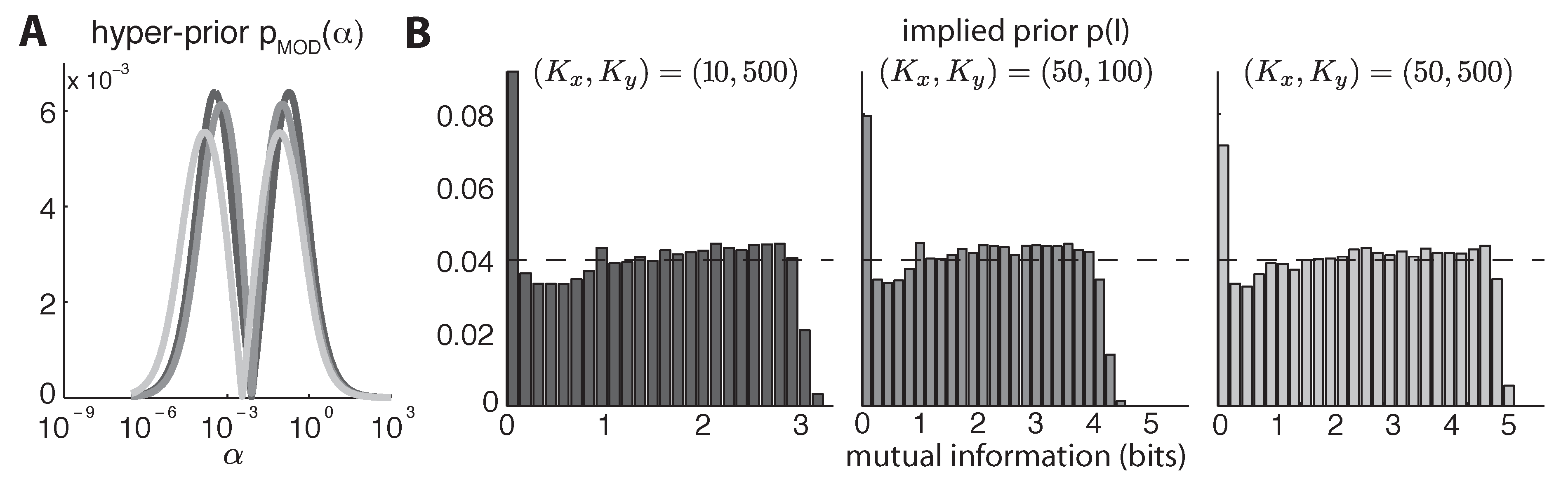
5.2. Mixture-of-Dirichlets (MOD) Prior

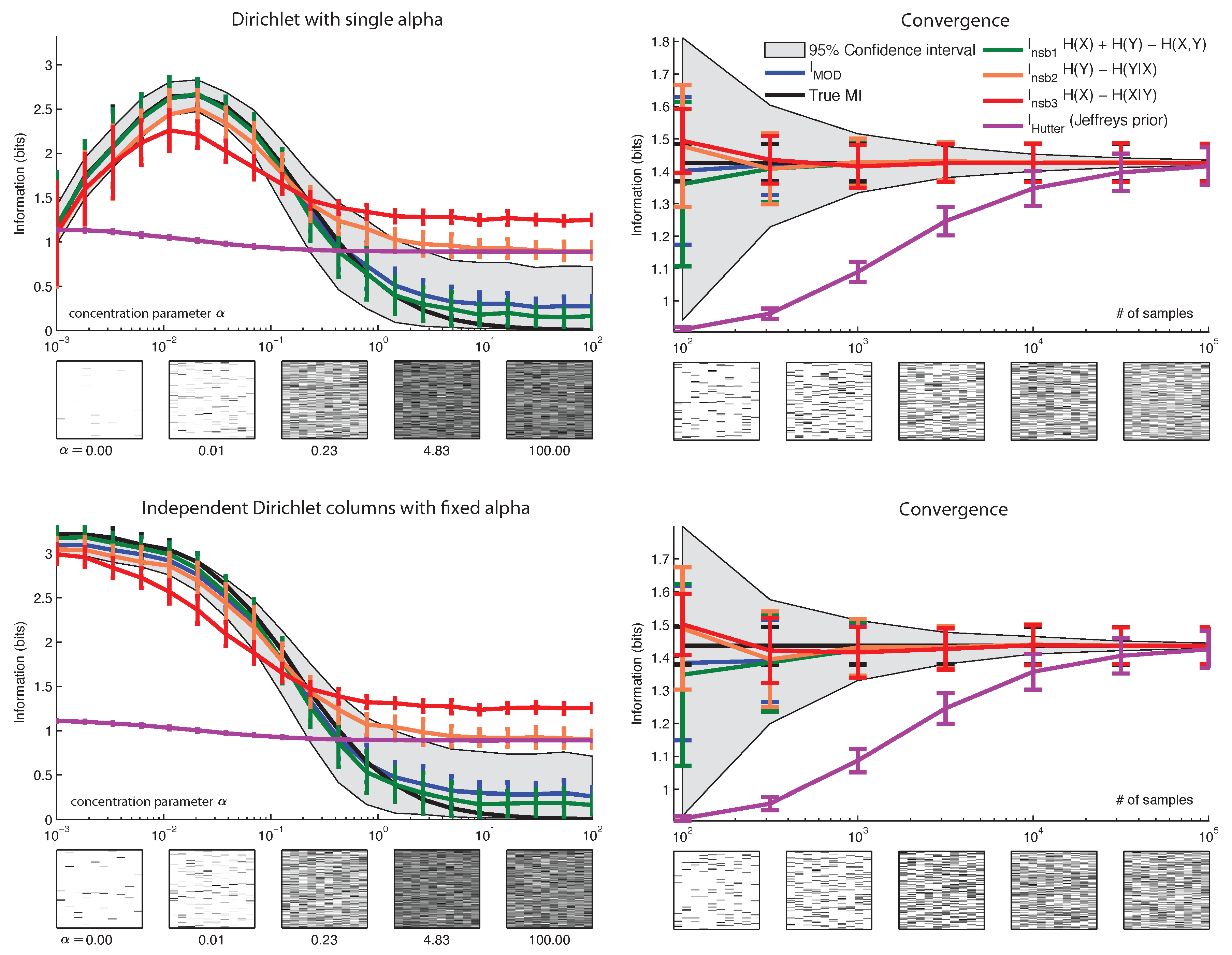
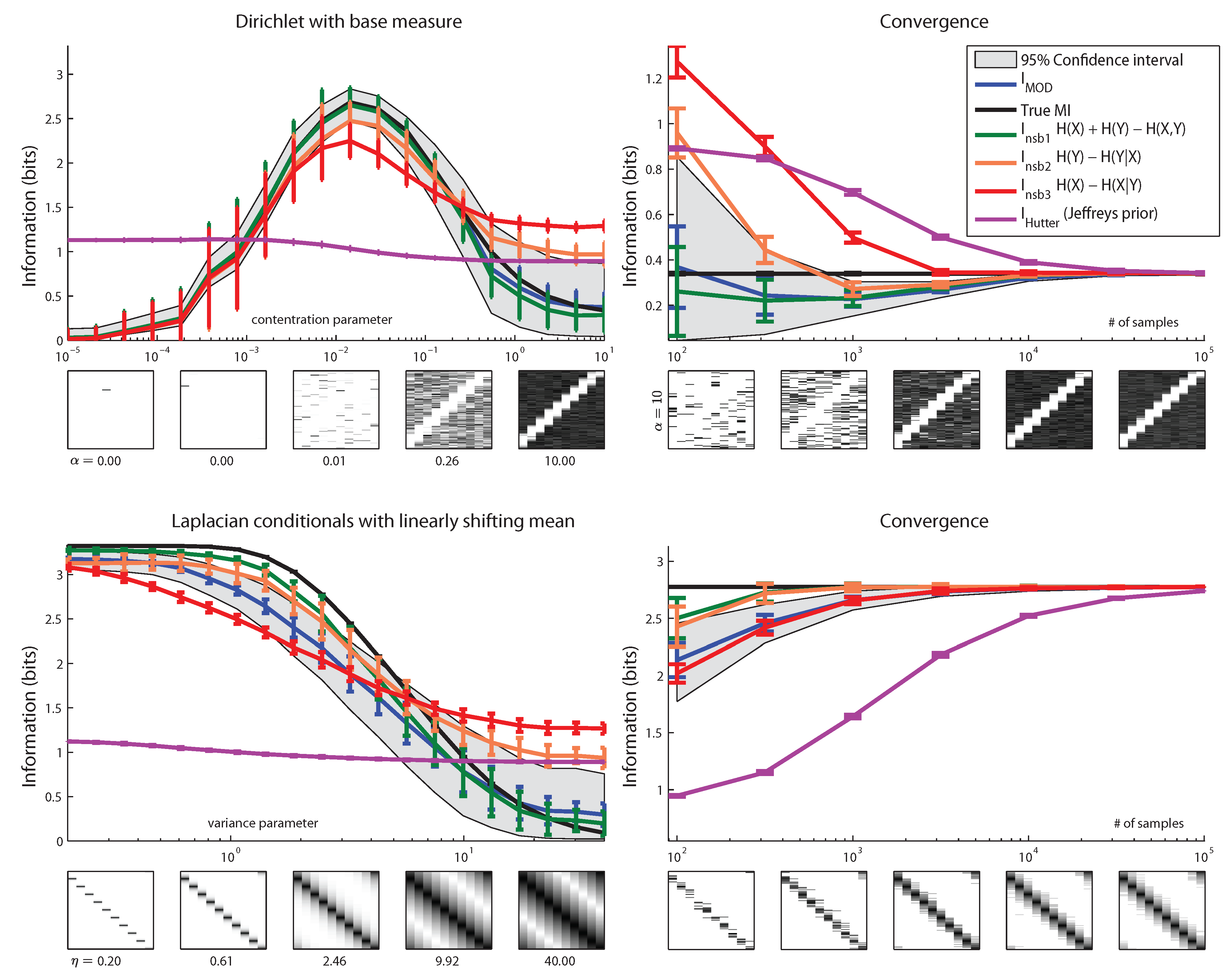
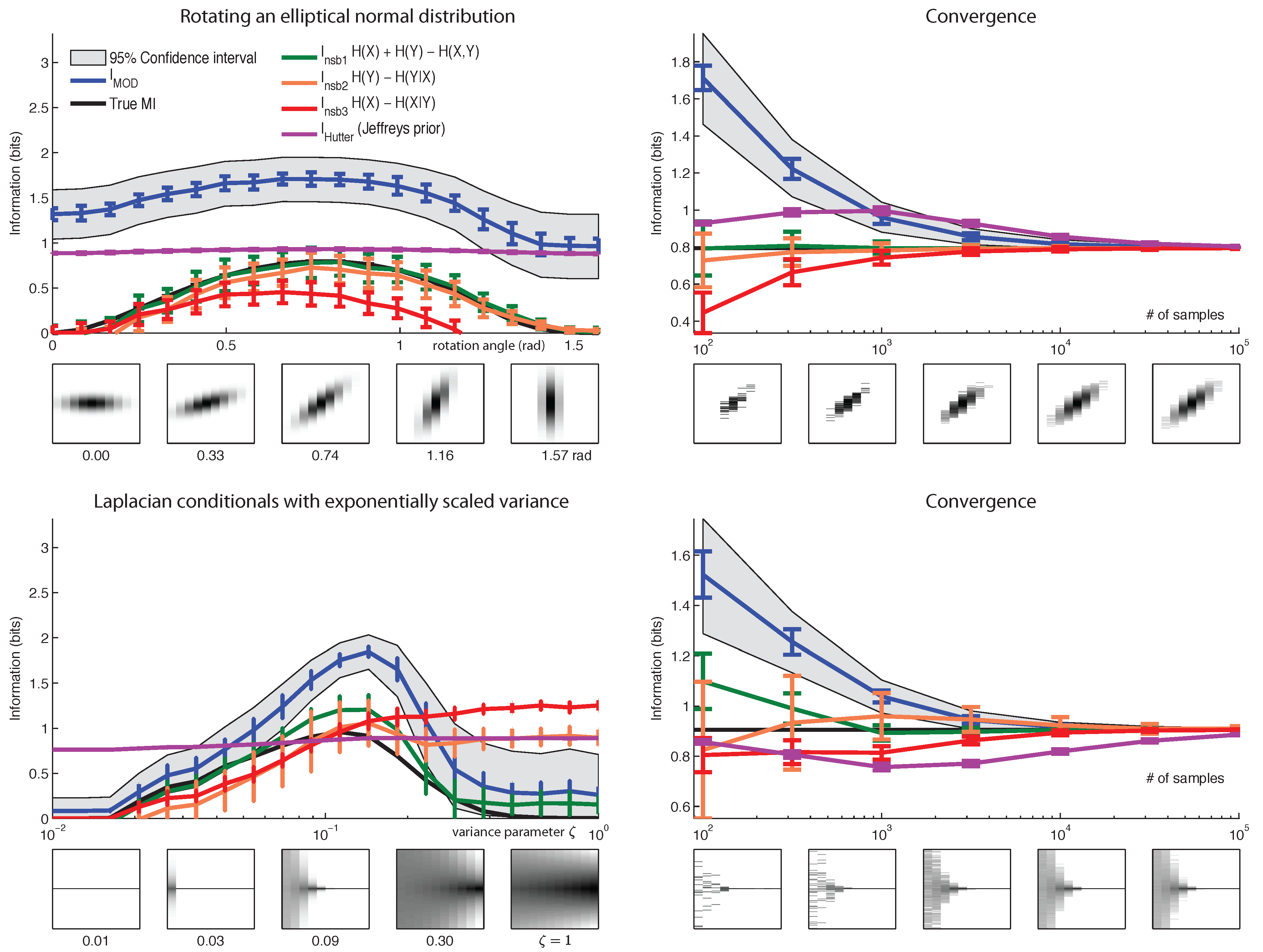
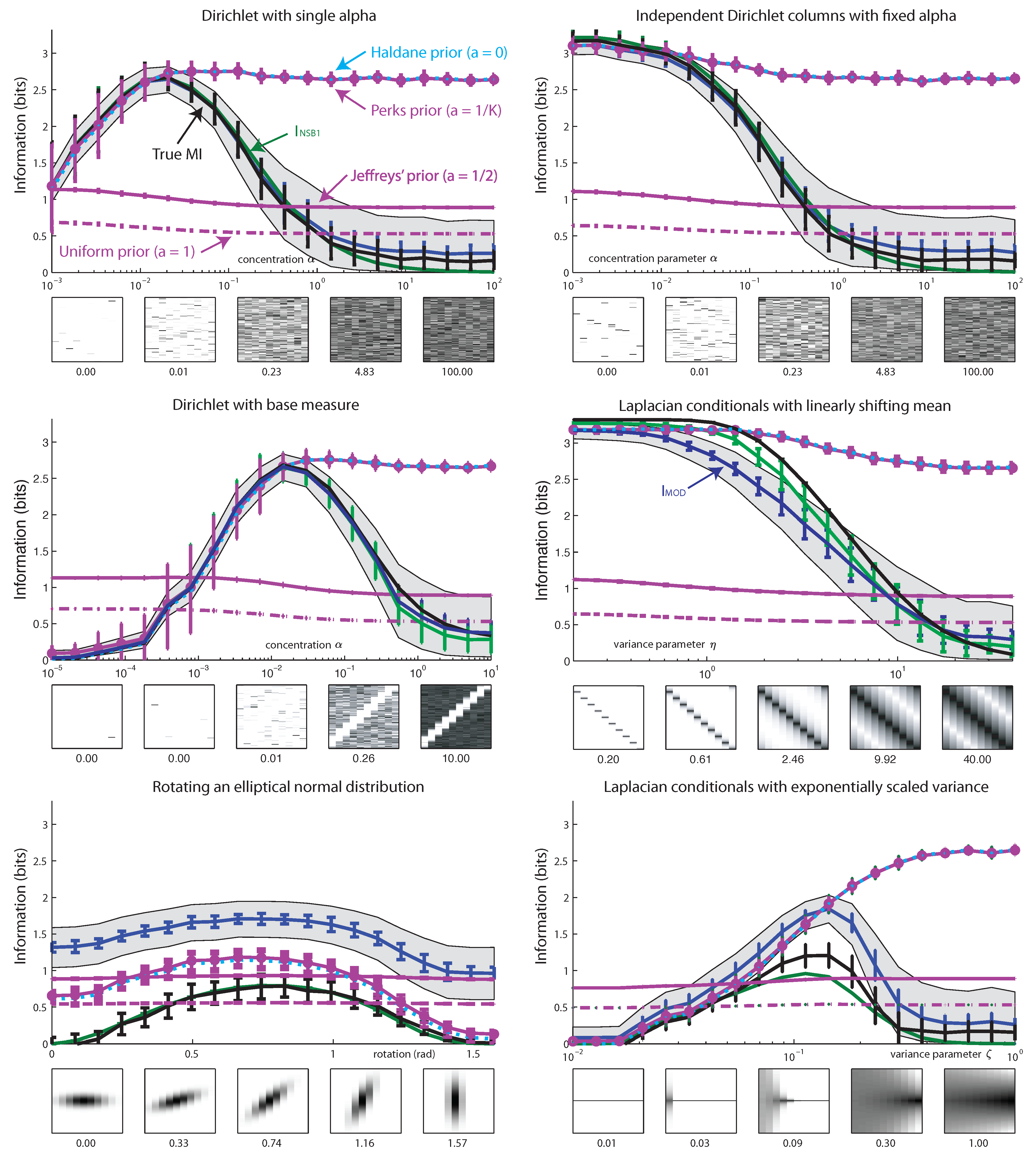
Following [17], we can design an approximately uniform NSB-style prior over MI by mixing together Dirichlet distributions with appropriate mixing weights. The posterior mean of mutual information under such a mixture prior will have a form directly analogous to Equation (10), except that the posterior mean of entropy is replaced by the posterior mean of MI (Equation (22)). We refer to the the resulting prior as the Mixture of Dirichlets (MOD) distribution. Naively, we want mixing weights to be proportional to the derivative of the expected MI with respect to α, which depends $K_x$ and $K_y$:

$$p_{\text{MOD}}(\alpha )\propto \frac{d}{d\alpha }\mathbb{E}\left[I(\pi )\right|\alpha ]=\frac{1}{ln2}\left[K{\psi }_1(K\alpha +1)+{\psi }_1(\alpha +1)-K_x{\psi }_1(K_x\alpha +1)-K_y{\psi }_1(K_y\alpha +1)\right].$$

(23)

However, this derivative crosses zero and becomes negative above some value ${\alpha }_0$, meaning we cannot simply normalize by ${\int }_0^{\infty }\frac{d}{d\alpha }\mathbb{E}\left[I(\pi )\right|\alpha ]d\alpha$ to obtain the prior. We are, however, free to weight $p_{\text{MOD}}(\alpha )$ for $\alpha \le {\alpha }_0$ and $\alpha \ge {\alpha }_0$ separately, to form a flat implied prior over I, since either side provides a flat prior. Our only constraint is that together they form a valid probability distribution (one might consider improper priors on α, but we do not pursue them here). We choose to combine the two portions together with equal weight, i.e., ${\int }_0^{{\alpha }_0}{p}_{\text{MOD}}(\alpha )d\alpha ={\int }_{{\alpha }_0}^{\infty }{p}_{\text{MOD}}(\alpha )d\alpha =\frac{1}{2}$. Empirically, we found different weightings of the two sides to give nearly identical performance. The result is a bimodal prior over α designed to provide an approximately uniform prior $p(I)$. (See Figure 5). Although the induced prior over I is not exactly uniform, it is relatively non-informative and robust to changes in table size. This represents a significant improvement over the fixed-α priors considered by [18]. However, the prior still assigns very little probability to distributions having the values of MI near the theoretical maximum. This roll-off in the prior near the maximum depends on the size of the matrix, and cannot be entirely overcome with any prior defined as a mixture of Dirichlet distributions.

Figure 5. Illustration of Mixture-of-Dirichlets (MOD) priors and hyper-priors, for three settings of $K_y$ and $K_x$. (A) Hyper-priors over α for three different-sized joint distributions: $(K_x,K_y)=(10,500)$ (dark), $(K_x,K_y)=(50,100)$ (gray), and $(K_x,K_y)=(50,500)$ (light gray). (B) Prior distributions over mutual information implied by each of the priors on α shown in (A). The prior on mutual information remains approximately flat for varying table sizes, but note that it does not assign very much probability the maximum possible mutual information, which is given by the right-most point on the abscissa in each graph.

Figure 5. Illustration of Mixture-of-Dirichlets (MOD) priors and hyper-priors, for three settings of $K_y$ and $K_x$. (A) Hyper-priors over α for three different-sized joint distributions: $(K_x,K_y)=(10,500)$ (dark), $(K_x,K_y)=(50,100)$ (gray), and $(K_x,K_y)=(50,500)$ (light gray). (B) Prior distributions over mutual information implied by each of the priors on α shown in (A). The prior on mutual information remains approximately flat for varying table sizes, but note that it does not assign very much probability the maximum possible mutual information, which is given by the right-most point on the abscissa in each graph.

6. Results

We analyzed the empirical performance of Bayesian (${\widehat{I}}_{\text{MOD}}$, ${\widehat{I}}_{\text{Hutter}}$) and quasi-Bayesian (${\widehat{I}}_{\text{NSB1}}$, ${\widehat{I}}_{\text{NSB2}}$, and ${\widehat{I}}_{\text{NSB3}}$) estimators on simulated data from six different joint distributions (shown in Figure 6, Figure 7, Figure 8 and Figure 9). We examine ${\widehat{I}}_{\text{Hutter}}$ with four fixed values of $\alpha =\{0,\frac{1}{K},\frac{1}{2},1\}$, with $K=K_x{K}_y$, as suggested in [19]. For visual simplicity, we show only the uninformative Jeffreys’ prior $\alpha =\frac{1}{2}$ in Figure 6, Figure 7 and Figure 8, and compare all other values in Figure 9. The conditional entropies appearing in ${\widehat{I}}_{\text{NSB2}}$ and ${\widehat{I}}_{\text{NSB3}}$ require estimates of the marginal distributions ${\pi }_y$ and ${\pi }_x$, respectively. We ran experiments using both the true marginal distributions ${\pi }_x$ and ${\pi }_y$ and their maximum likelihood (plugin) estimates from data. The two cases showed little difference in the experiments shown here (data not shown). Note that all these estimators are consistent, as illustrated in the convergence figures (right column in Figure 6, Figure 7 and Figure 8). However, with a small number of samples, the estimators exhibited substantial bias (left column).

Figure 6. Performance of MI estimators for true distributions sampled from distributions related to Dirichlet. Joint distributions have 10 × 100 bins. (left column) Estimated mutual information from 100 data samples, as a function of a parameter defining the true distribution. Error bars indicate the variability of the estimator over independent samples (± one standard deviation). Gray shading denotes the average 95% Bayesian credible interval. Insets show examples of true joint distributions, for visualization purposes. (right column) Convergence as a function of sample size. True distribution is given by that shown in the central panel of the corresponding figure on the left. Inset images show examples of empirical distribution, calculated from data. (top row) True distributions sampled from a fixed Dirichlet Dir(α) prior, where α varies from 10⁻³ to 10². (bottom row) Each column (conditional) is an independent Dirichlet distribution with a fixed α.

Figure 6. Performance of MI estimators for true distributions sampled from distributions related to Dirichlet. Joint distributions have 10 × 100 bins. (left column) Estimated mutual information from 100 data samples, as a function of a parameter defining the true distribution. Error bars indicate the variability of the estimator over independent samples (± one standard deviation). Gray shading denotes the average 95% Bayesian credible interval. Insets show examples of true joint distributions, for visualization purposes. (right column) Convergence as a function of sample size. True distribution is given by that shown in the central panel of the corresponding figure on the left. Inset images show examples of empirical distribution, calculated from data. (top row) True distributions sampled from a fixed Dirichlet Dir(α) prior, where α varies from 10⁻³ to 10². (bottom row) Each column (conditional) is an independent Dirichlet distribution with a fixed α.

Figure 7. Performance of MI estimators on distributions sampled from more structured distributions. Joint distributions have 10 × 100 bins. The format of left and right columns is the same as in Figure 6. (top row) Dirichlet joint distribution with a base measure ${\mu }_{ij}$ chosen such that there is a diagonal strip of low concentration. The base measure is given by ${\mu }_{ij}\propto \frac{1}{{10}^{-6}+Q(i,j)}$, where $Q(x,y)$ is a $2D$ Gaussian probability density function with 0 mean and covariance matrix $\left[\begin{array}{cc}0.08& 0\\ 0& 0.0003\end{array}\right]$. We normalized ${\mu }_{ij}$ to sum to one over the grid shown. (bottom row) Laplace conditional distributions with linearly-shifting means. Each conditional $p(Y=y|X=x)$ has the form of $e^{-|y-10x|/\eta }$. These conditionals are shifted circularly with respect to one another, generating a diagonal structure.

Figure 7. Performance of MI estimators on distributions sampled from more structured distributions. Joint distributions have 10 × 100 bins. The format of left and right columns is the same as in Figure 6. (top row) Dirichlet joint distribution with a base measure ${\mu }_{ij}$ chosen such that there is a diagonal strip of low concentration. The base measure is given by ${\mu }_{ij}\propto \frac{1}{{10}^{-6}+Q(i,j)}$, where $Q(x,y)$ is a $2D$ Gaussian probability density function with 0 mean and covariance matrix $\left[\begin{array}{cc}0.08& 0\\ 0& 0.0003\end{array}\right]$. We normalized ${\mu }_{ij}$ to sum to one over the grid shown. (bottom row) Laplace conditional distributions with linearly-shifting means. Each conditional $p(Y=y|X=x)$ has the form of $e^{-|y-10x|/\eta }$. These conditionals are shifted circularly with respect to one another, generating a diagonal structure.

Among Bayesian estimators, we found ${\widehat{I}}_{\text{MOD}}$ performed substantially better than ${\widehat{I}}_{\text{Hutter}}$ in almost all cases. However, we found that quasi-Bayesian estimators generally outperformed the fully Bayesian estimators, and ${\widehat{I}}_{\text{NSB1}}$ exhibited the best performance overall. The ${\widehat{I}}_{\text{MOD}}$ estimator performed well when the joint distribution π was drawn from a Dirichlet distribution with a fixed α (Figure 6 top). It also performed well when each column was independently distributed as Dirichlet with a constant global α (Figure 6 bottom). The ${\widehat{I}}_{\text{Hutter}}$ estimator performed poorly except when the true concentration parameter matched the value assumed by the estimator ($\alpha =\frac{1}{2}$). Among the quasi-Bayesian estimators, ${\widehat{I}}_{\text{NSB1}}$ had the best performance, on par with ${\widehat{I}}_{\text{MOD}}$.

Figure 8. Performance of MI estimators: failure mode for ${\widehat{I}}_{\text{MOD}}$. Joint distributions have 10 × 100 bins. The format of left and right column is same as in Figure 6. (top row) True distributions are rotating, discretized Gaussians, where rotation angle is varied from 0 to π. For cardinal orientations, the distribution is independent and MI is 0. For diagonal orientations, the MI is maximal. (bottom row) Each column (conditional) is an independent Laplace (double-exponential) distribution: $p(Y=j|X=i)=e^{-|j-50|/\tau (i)}$. The width of the Laplace distribution is governed by $\tau (i)=e^{-1.11i\zeta }$ where ζ is varied from 10⁻² to 1.

Figure 8. Performance of MI estimators: failure mode for ${\widehat{I}}_{\text{MOD}}$. Joint distributions have 10 × 100 bins. The format of left and right column is same as in Figure 6. (top row) True distributions are rotating, discretized Gaussians, where rotation angle is varied from 0 to π. For cardinal orientations, the distribution is independent and MI is 0. For diagonal orientations, the MI is maximal. (bottom row) Each column (conditional) is an independent Laplace (double-exponential) distribution: $p(Y=j|X=i)=e^{-|j-50|/\tau (i)}$. The width of the Laplace distribution is governed by $\tau (i)=e^{-1.11i\zeta }$ where ζ is varied from 10⁻² to 1.

In Figure 7, the joint distributions significantly deviate from the prior assumed by the ${\widehat{I}}_{\text{MOD}}$ estimator. The top panel shows joint distributions sampled from a Dirichlet distribution with non-constant concentration parameter, taking the form $\text{Dir}(\alpha {\mu }_{11},\alpha {\mu }_{12},\dots ,\alpha {\mu }_{K_x{K}_y})$, with variable weights ${\mu }_{ij}$. The bottom panel shows joint distributions defined by double-exponential distributions in each column. Here, the ${\widehat{I}}_{\text{MOD}}$ estimator exhibits reasonable performance, and ${\widehat{I}}_{\text{NSB1}}$ is the best quasi-Bayesian estimator.

Figure 8 shows two example distributions for which ${\widehat{I}}_{\text{MOD}}$ performs relatively poorly, yet the quasi-Bayesian estimators perform well. These joint distributions have low probability in the space parameterized by a Dirichlet distribution with fixed α parameter. As a result, when data are drawn from such distributions, ${\widehat{I}}_{\text{MOD}}$ posterior estimates are far removed from the true mutual information.

Figure 9. Comparison of Hutter MI estimator for different values of α. Four datasets shown in Figure 6 and Figure 7 are used with the same sample size of N = 0. We compare improper Haldane prior (α = 0), Perks prior ($\alpha =\frac{1}{K_x{K}_y}$), Jeffreys’ prior ($\alpha =\frac{1}{2}$), and uniform prior (α = 1) [19]. ${\widehat{I}}_{\text{NSB1}}$ is also shown for comparison.

Figure 9. Comparison of Hutter MI estimator for different values of α. Four datasets shown in Figure 6 and Figure 7 are used with the same sample size of N = 0. We compare improper Haldane prior (α = 0), Perks prior ($\alpha =\frac{1}{K_x{K}_y}$), Jeffreys’ prior ($\alpha =\frac{1}{2}$), and uniform prior (α = 1) [19]. ${\widehat{I}}_{\text{NSB1}}$ is also shown for comparison.

Among the quasi-Bayesian estimators, ${\widehat{I}}_{\text{NSB1}}$ had superior performance compared to both ${\widehat{I}}_{\text{NSB2}}$ and ${\widehat{I}}_{\text{NSB3}}$, for all of the examples we considered. To our knowledge, ${\widehat{I}}_{\text{NSB1}}$ is not used in the literature, and this comparison between different forms of NSB estimation has not been shown previously. However, the quasi-Bayesian estimators sometimes give negative estimates of mutual information, for example in the rotating Gaussian distribution (see Figure 8, upper left).

In Figure 9, we examined the performance of ${\widehat{I}}_{\text{Hutter}}$ for these same simulated datasets, for several different commonly-used values of the Dirichlet parameter α [19]. The ${\widehat{I}}_{\text{Hutter}}$ estimate under Jeffrey’s ($\alpha =\frac{1}{2}$) and Uniform (α = 1) priors is highly determined by the prior, and does not track the true entropy accurately. However, the ${\widehat{I}}_{\text{Hutter}}$ estimate with smaller α (Haldane and Perks priors) exhibits reasonably good performance across a range of values of the true entropy, as long as the true distribution is relatively sparse. This indicates that small-α Dirichlet priors are less informative about mutual information than large-α priors (which may also be observed from the gray regions in Figure 4 showing quantiles of I|α).

7. Conclusions

We have proposed ${\widehat{I}}_{\text{MOD}}$, a novel Bayesian mutual information estimator that uses a mixture-of-Dirichlets prior over the space of joint discrete probability distributions. We designed the mixing distribution to achieve an approximately flat prior over MI, following a strategy similar to the one proposed by [17] in the context of entropy estimation. However, we find that the MOD estimator exhibits relatively poor empirical performance compared with quasi-Bayesian estimators, which rely on combinations Bayesian entropy estimates. This suggests that mixtures of Dirichlet priors do not provide a flexible enough family of priors for highly-structured joint distributions, at least for purposes of MI estimation.

However, quasi-Bayesian estimators based on NSB entropy estimates exhibit relatively high accuracy, particularly the form denoted ${\widehat{I}}_{\text{NSB1}}$, which involves the difference of marginal and joint entropy estimates. The neuroscience literature has typically employed ${\widehat{I}}_{\text{NSB3}}$, but our simulations suggests ${\widehat{I}}_{\text{NSB1}}$ may perform better. Nevertheless, quasi-Bayesian estimators also show significant failure modes. These problems arise from its use of distinct models for the marginals and conditionals of a joint distribution, which do not correspond to a coherent prior over the joint. This suggests an interesting direction for future research: to develop a well-formed prior over joint distributions that harnesses the good performance of quasi-Bayesian estimators while producing a tractable Bayesian least squares estimator, providing reliable Bayesian credible intervals while avoiding pitfalls such as negative estimates.

While the properties of the Dirichlet prior, in particular the closed form of $\mathbb{E}\left[I\right|\alpha ]$, make the MOD estimator tractable and easy to compute, one might consider more flexible models that rely on sampling for inference. A natural next step would be to design a prior capable of mimicking the performance of ${\widehat{I}}_{\text{NSB1}}$, ${\widehat{I}}_{\text{NSB2}}$, or ${\widehat{I}}_{\text{NSB3}}$ under fully Bayesian sampling-based inference.

References

1. Schindler, K.H.; Palus, M.; Vejmelka, M.; Bhattacharya, J. Causality detection based on information-theoretic approaches in time series analysis. Phys. Rep. 2007, 441, 1–46. [Google Scholar]
2. Rényi, A. On measures of dependence. Acta Math. Hung. 1959, 10, 441–451. [Google Scholar] [CrossRef]
3. Chow, C.; Liu, C. Approximating discrete probability distributions with dependence trees. Inf. Theory IEEE Trans. 1968, 14, 462–467. [Google Scholar] [CrossRef]
4. Rieke, F.; Warland, D.; de Ruyter van Steveninck, R.; Bialek, W. Spikes: Exploring the Neural Code; MIT Press: Cambridge, MA, USA, 1996. [Google Scholar]
5. Ma, S. Calculation of entropy from data of motion. J. Stat. Phys. 1981, 26, 221–240. [Google Scholar] [CrossRef]
6. Bialek, W.; Rieke, F.; de Ruyter van Steveninck, R.R.; Warland, D. Reading a neural code. Science 1991, 252, 1854–1857. [Google Scholar] [CrossRef] [PubMed]
7. Strong, S.; Koberle, R.; de Ruyter van Steveninck, R.; Bialek, W. Entropy and information in neural spike trains. Phys. Rev. Lett. 1998, 80, 197–202. [Google Scholar] [CrossRef]
8. Paninski, L. Estimation of entropy and mutual information. Neural Comput. 2003, 15, 1191–1253. [Google Scholar] [CrossRef]
9. Barbieri, R.; Frank, L.; Nguyen, D.; Quirk, M.; Solo, V.; Wilson, M.; Brown, E. Dynamic Analyses of Information Encoding in Neural Ensembles. Neural Comput. 2004, 16, 277–307. [Google Scholar] [CrossRef] [PubMed]
10. Kennel, M.; Shlens, J.; Abarbanel, H.; Chichilnisky, E. Estimating Entropy Rates with Bayesian Confidence Intervals. Neural Comput. 2005, 17, 1531–1576. [Google Scholar] [CrossRef] [PubMed]
11. Victor, J. Approaches to information-theoretic analysis of neural activity. Biol. Theory 2006, 1, 302–316. [Google Scholar] [CrossRef] [PubMed]
12. Shlens, J.; Kennel, M.B.; Abarbanel, H.D.I.; Chichilnisky, E.J. Estimating information rates with confidence intervals in neural spike trains. Neural Comput. 2007, 19, 1683–1719. [Google Scholar] [CrossRef] [PubMed]
13. Vu, V.Q.; Yu, B.; Kass, R.E. Coverage-adjusted entropy estimation. Stat. Med. 2007, 26, 4039–4060. [Google Scholar] [CrossRef] [PubMed]
14. Montemurro, M.A.; Senatore, R.; Panzeri, S. Tight data-robust bounds to mutual information combining shuffling and model selection techniques. Neural Comput. 2007, 19, 2913–2957. [Google Scholar] [CrossRef] [PubMed]
15. Vu, V.Q.; Yu, B.; Kass, R.E. Information in the Nonstationary Case. Neural Comput. 2009, 21, 688–703. [Google Scholar] [CrossRef] [PubMed]
16. Archer, E.; Park, I.M.; Pillow, J. Bayesian estimation of discrete entropy with mixtures of stick-breaking priors. In Advances in Neural Information Processing Systems 25; Bartlett, P., Pereira, F., Burges, C., Bottou, L., Weinberger, K., Eds.; MIT Press: Cambridge, MA, 2012; pp. 2024–2032. [Google Scholar]
17. Nemenman, I.; Shafee, F.; Bialek, W. Entropy and inference, revisited. In Advances in Neural Information Processing Systems 14; MIT Press: Cambridge, MA, 2002; pp. 471–478. [Google Scholar]
18. Hutter, M. Distribution of mutual information. In Advances in Neural Information Processing Systems 14; MIT Press: Cambridge, MA, 2002; pp. 399–406. [Google Scholar]
19. Hutter, M.; Zaffalon, M. Distribution of mutual information from complete and incomplete data. Comput. Stat. Data Anal. 2005, 48, 633–657. [Google Scholar] [CrossRef]
20. Treves, A.; Panzeri, S. The upward bias in measures of information derived from limited data samples. Neural Comput. 1995, 7, 399–407. [Google Scholar] [CrossRef]
21. Wolpert, D.; Wolf, D. Estimating functions of probability distributions from a finite set of samples. Phys. Rev. E 1995, 52, 6841–6854. [Google Scholar] [CrossRef]
22. Minka, T. Estimating a Dirichlet Distribution; Technical report; MIT: Cambridge, MA, USA, 2003. [Google Scholar]
23. Nemenman, I.; Lewen, G.D.; Bialek, W.; de Ruyter van Steveninck, R.R. Neural coding of natural stimuli: information at sub-millisecond resolution. PLoS Comput. Biol. 2008, 4, e1000025. [Google Scholar] [CrossRef] [PubMed]