Article

Zero Delay Joint Source Channel Coding for Multivariate Gaussian Sources over Orthogonal Gaussian Channels

1
Intervention Center, Oslo University Hospital and Institute of Clinical Medicine, University of Oslo,0372 Oslo, Norway
2
Department of Electronics and Telecommunication, Norwegian University of Science and Technology (NTNU), 7491 Trondheim, Norway
3
SINTEF ICT, Forskningsveien 1, 0314 Oslo, Norway
*
Authors to whom correspondence should be addressed.
Entropy 2013, 15(6), 2129-2161; https://doi.org/10.3390/e15062129
Submission received: 26 April 2013 / Revised: 18 May 2013 / Accepted: 21 May 2013 / Published: 31 May 2013

Abstract

:
Communication of a multivariate Gaussian source transmitted over orthogonal additive white Gaussian noise channels using delay-free joint source channel codes (JSCC) is studied in this paper. Two scenarios are considered: (1) all components of the multivariate Gaussian are transmitted by one encoder as a vector or several ideally collaborating nodes in a network; (2) the multivariate Gaussian is transmitted through distributed nodes in a sensor network. In both scenarios, the goal is to recover all components of the multivariate Gaussian at the receiver. The paper investigates a subset of JSCC consisting of direct source-to-channel mappings that operate on a symbol-by-symbol basis to ensure zero coding delay. A theoretical analysis that helps explain and quantify distortion behavior for such JSCC is given. Relevant performance bounds for the network are also derived with no constraints on complexity and delay. Optimal linear schemes for both scenarios are presented. Results for Scenario 1 show that linear mappings perform well, except when correlation is high. In Scenario 2, linear mappings provide no gain from correlation when the channel signal-to-noise ratio (SNR) gets large. The gap to the performance upper bound is large for both scenarios, regardless of SNR, when the correlation is high. The main contribution of this paper is the investigation of nonlinear mappings for both scenarios. It is shown that nonlinear mappings can provide substantial gain compared to optimal linear schemes when correlation is high. Contrary to linear mappings for Scenario 2, carefully chosen nonlinear mappings provide a gain for all SNR, as long as the correlation is close to one. Both linear and nonlinear mappings are robust against variations in SNR.

1. Introduction

We study the problem of transmitting a multivariate Gaussian source over orthogonal additive white Gaussian noise channels with joint source channel codes (JSCC), where the source and channel dimensions, M, are equal. We place special emphasis on delay-free codes. That is, we require the JSCC to operate on a symbol-by-symbol basis. Two scenarios are considered: (1) the multivariate Gaussian is communicated as an M-dimensional vector source by one encoder over M parallel channels or M channel uses. This scenario can also be seen as ideally collaborating nodes in a network (“Ideal collaboration" means that all nodes have access to a noiseless version of all the other node observations without any additional cost), communicating over equal and independent channels (see Figure 1a). (2) The multivariate Gaussian is communicated as M distributed (i.e., non-collaborating) sensor nodes with correlated measurements in a sensor network. That is, each node encodes one component of the multivariate Gaussian (see Figure 1b). Scenario 2 can be seen as a special case of Scenario 1. In a more practical setting, Scenarios 1 and 2 may, for instance, represent several wired or non-wired in- or on-body sensors in a body area network communicating with a common off-body receiver.
Figure 1. Block diagram for networks under consideration. (a) Scenario 1: cooperative encoders; (b) Scenario 2: distributed encoders.
Entropy 15 02129 g001
Communication problems of this nature have been investigated for several decades. For lossless channels, it was proven in [1] that distributed lossless coding of finite alphabet correlated sources can be as rate efficient as with full collaboration between the sensor nodes. This result assumes no restriction on complexity and delay. It is not known whether a similar conclusion holds in the finite complexity and delay regime. For lossy source coding of a Gaussian vector source (Scenario 1), the rate-distortion function was determined in [2]. For lossy distributed source coding (Scenario 2), the rate-distortion function for recovering information common to all sources was solved in [3]. For the case of recovering Gaussian sources (both common, as well as individual information) from two terminals, the exact rate-distortion region was determined by [4,5]. The multi-terminal rate-distortion region is still unknown, although several efforts towards a solution have been made in [4,6].
If the channel between the source and sink is lossy, system performance is generally evaluated in terms of tradeoffs between cost on the channel, for example, transmit power, and the end-to-end distortion of the source. Considering Scenario 1, the bounds can be found by equating the rate-distortion function for vector sources with the Gaussian channel capacity. These bounds can be achieved by separate source and channel coding (SSCC), assuming infinite complexity and delay. Considering Scenario 2, the bound is determined, in the case of two sensor nodes, by combining the rate-distortion region in [4,5] with the Gaussian channel capacity. This bound is achieved through SSCC by vector quantizing each source, then applying Slepian-Wolf coding [1], followed by capacity achieving channel codes [7].
Optimality of the aforementioned SSCC schemes comes at the expense of complexity and infinite coding delays. If the application has low complexity and delay requirements, it may be beneficial to apply JSCC. Several such schemes have been investigated in the literature: For Scenario 2, a simple nonlinear zero delay JSCC scheme for transmitting a single random variable observed by several noisy sensor measurements over a noisy wireless channel was suggested in [8]. Similar JSCC schemes for communication of two or more correlated Gaussian random variables over wireless noisy channels was proposed and optimized in [9]. An extension of the scheme suggested in [8] using multidimensional lattices to code blocks of samples proposed in [10]. Further, [11] found similar JSCC using variational calculus and [12] introduced a distributed Karhunen-Loève transform. The authors of [13] examined Scenario 2, also with side information available at both encoder and decoder. A similar problem with non-orthogonal access on the channel was studied in [14,15]. At the moment, we do not know of any efforts specifically targeting delay-free JSCC for Scenario 1, although all schemes for Scenario 2 apply as special cases. Optimal linear solutions for this problem may be found from [16].
In this paper, we utilize a subset of JSCC named Shannon-Kotelnikov mappings (S-K Mappings), built on ideas from earlier efforts [16,17,18,19,20,21,22,23,24,25,26,27,28,29,30]. S-K mappings are continuous or piecewise continuous direct source-to-channel mappings that operate directly on continuous amplitude, discrete time signals and have shown excellent performance for the point-to-point problem with independent and identically distributed (i.i.d.) sources [27,30,31,32,33,34,35]. Such mappings were applied for multiple description JSCC for wireless channels in [36]. A semi-analog approach without restriction on complexity and delay, also treating colored sources and channels, was given in [37].
A theoretical analysis that helps explain and quantify distortion behavior for such mappings is given in this paper. We investigate Scenario 1 as a generalization of our previous work in [31,32,38] on dimension expanding S-K mappings for i.i.d. sources, by including arbitrary correlation. Similarly, we study Scenario 2 by extending the use of S-K mappings to a network of non-collaborating nodes with inter-correlated observations. Properly designed JSCC schemes for Scenario 1 may serve as bounds for schemes developed for Scenario 2, since Scenario 1 has more degrees of freedom in constructing encoding operations. The treatment of Scenario 2 also seeks to explain why certain existing JSCC solutions for this problem (like the ones in [9]) are configured the way they are and also suggests schemes that can offer better performance in certain cases. Throughout this paper, Scenarios 1 and 2 will often be referred to as collaborative case and distributed case, respectively.
The paper is organized as follows: In Section 2, we formulate the problem and derive performance bounds assuming arbitrary code lengths. These bounds are achievable in Scenario 1 and serve as upper bounds on performance for Scenario 2. In Section 3, we analyze optimal linear mappings and discuss under what conditions it is meaningful to apply linear schemes. In Section 4, we introduce nonlinear mappings. We revisit some results from [8,31,32,38] in order to mathematically formulate the problem and give examples on and optimize selected mappings. In Section 5, we summarize and conclude.
Note that parts of this paper have previously been published in [39]. Results on nonlinear mappings in Section 4 are mostly new and constitute the main contribution of the paper.

2. Problem Formulation and Performance Bounds

The communication system studied in this paper is depicted in Figure 1.
M correlated sources, x 1 , x 2 , . . . x M , are encoded by M functions and transmitted on M orthogonal channels.
The sources have a common information, y, and an (additive) independent component, z 1 , z 2 , . . . z M , that is x m = y + z m , m = { 1 , 2 , . . . M } . Furthermore, both y and z m are discrete time, continuous amplitude, memoryless Gaussian random variables, of zero mean and variances σ y 2 and σ z m 2 , respectively, and x 1 , x 2 , . . . x M are conditionally independent, given y. The correlation coefficient between any pair of sources, m , k , is then ρ m , k = σ y 2 / σ x m σ x k , m k , where σ x m 2 is the variance of source m and σ x m 2 = σ y 2 + σ z m 2 . With all observations collected in the vector x = [ x 1 , x 2 , , x M ] T , the joint probability density function (pdf) is given by:
p x ( x ) = 1 ( 2 π ) M det ( C x ) e - 1 2 x T C x - 1 x
where C x = E { x x T } is the covariance matrix.
Two scenarios are considered: (1) Each encoding function operates on all variables, f m ( x 1 , x 2 , , x M ) , as in Figure 1a. This scenario can be seen as one encoder operating on an M dimensional vector source or as M ideally collaborating encoders. (2) Each encoder operates on one variable, f m ( x m ) , m = 1 , , M , as in Figure 1b. This scenario can be seen as M non-collaborating nodes in a sensor network. The encoders operate independently, but are jointly optimized. Throughout the rest of the paper, we refer to Scenario 1 as collaborative case, and Scenario 2 as distributed case.
The encoded observations are transmitted over M-independent, additive white Gaussian noise (AWGN) channels with noise n N ( 0 , σ n 2 I ) , where I is the identity matrix. For the distributed case, we impose an average transmit power constraint, P m , for each node, m, where:
E { f m 2 } P m , m = { 1 , 2 , . . . M }
whereas in the collaborative case, we look at an average power constraint, P a , over all outputs, P a = ( P 1 + P 2 + + P M ) / M . These constraints are equal, if the power for all nodes is the same.
We will consider the special case where σ x 1 2 = σ x 2 2 = = σ x M 2 = σ x 2 . Then, ρ i j = ρ x = σ y 2 / σ x 2 , i , j and y N ( 0 , σ x 2 ρ x ) and z m N 0 , σ x 2 ( 1 - ρ x ) , m [ 1 , , M ] . For this special case, the covariance matrix is simple and has eigenvalues λ 1 > λ 2 = λ 3 = = λ M where λ 1 = σ x 2 ( M - 1 ) ρ x + 1 and λ m = σ x 2 ( 1 - ρ x ) , m [ 2 , , M ] . We restrict our investigation to this special case for the sake of simplicity and in order to achieve compact closed-form expressions. Generalization to networks with unequal transmit power and correlation can naturally be made.
At the receiver, the decoding functions, g m ( r 1 , r 2 , . . . r M ) , which have access to all received channel outputs, r 1 , r 2 , . . . r M , produce an estimate, x ^ m , of each source. We define the end-to-end distortion, D, as the mean-squared-error (MSE) averaged over all source symbols:
D = 1 M m = 1 M E { | x m - x ^ m | 2 } , m = { 1 , 2 , . . . M }
We assume ideal Nyquist sampling and ideal Nyquist channels, where the sampling rate of each source is the same as the signaling rate of each channel. We also assume ideal synchronization and timing in the network. Our design objective is to construct the encoding and decoding functions, f m and g m , that minimize D, subject to a transmit power constraint, P.

2.1. Distortion Bounds

Achievable bounds for the problem at hand can be derived for the cooperative case, and these serve as lower bounds for the distributed case. The achievable bound for the distributed case is currently only known when M = 2 , and was shown in [9] to be:
D dist = ( 1 + SNR ) - 2 ( 1 - ρ x 2 ) + ρ x 2 ( 1 + SNR ) - 4
where SNR = P / σ n 2 is the channel signal-to-noise ratio.
To derive bounds for general M, we consider ideal collaboration.
Proposition 1 Consider the network depicted in Figure 1. In the symmetric case, D 1 = D 2 = = D M = D with transmit power P 1 = P 2 = = P M = P and correlation ρ i j = ρ x , i , j , the smallest achievable distortion for Scenario 1 and the distortion lower bound for Scenario 2 is given by:
D σ x 2 1 M 1 + ( M - 1 ) ρ x ( SNR + 1 ) M + ( M - 1 ) ( 1 - ρ x ) , SNR 1 + ( M - 1 ) ρ x 1 - ρ x M - 1 ( 1 + ( M - 1 ) ρ x ) ( 1 - ρ x ) M - 1 M SNR + 1 , SNR > 1 + ( M - 1 ) ρ x 1 - ρ x M - 1
Proof 1 Let R * , D * and P * denote optimal rate, distortion and power, respectively. Assuming full collaboration, the M sources can be considered as a Gaussian vector source of dimension, M. Then from [2]:
D * ( θ , M ) = 1 M i = 1 M min [ θ , λ i ] , R * ( θ , M ) = 1 M i = 1 M max 0 , 1 2 log 2 λ i θ
where λ i is the i-th eigenvalue of the covariance matrix, C x . The channel is a memoryless Gaussian vector channel of dimension, M, with covariance matrix, σ n 2 I . Its capacity with power, M P * , per source vector, ( x 1 , x 2 , . . . x M ) , is:
C ( M P * ) = 1 2 log 2 1 + M P * M σ n 2 = 1 2 log 2 1 + P * σ n 2
Now equate R * from Equation (6) with C in Equation (7) and calculate the corresponding power, P * . We get D D * ( θ , M ) with D * given in Equation (6) and:
P = P * ( θ , M ) = σ n 2 i = 1 M max [ λ i / θ , 1 ] 1 / M - 1
The max and min in Equations (6) and (8) depend on ρ x and the SNR. Since the special case, ρ i j = ρ x , i , j , is treated, there are two cases to consider: only the first eigenvalue, λ 1 (the common information), or all eigenvalues, λ i , i [ 1 , M ] , are to be represented. By solving Equation (8) with respect to θ for these two cases and inserting the result into Equation (6), the bound in Equation (5) results. Finally, the validity of these two cases is found by solving the equation, λ i = θ [with θ in Equation (8)], with respect to SNR= P / σ n 2 . □
In the following sections, we will compare suggested mappings to OPTA coop = σ x 2 / D * (Optimal Performance Theoretically Attainable for the cooperative case), i.e., the best possible received signal-to-distortion ratio (SDR) as a function of SNR.
By comparing Equations (6) and (8) with Equation (4) (see Figure 2a), one can show that the above cooperative distortion bound is tight, even for the distributed case when channel SNR is high enough.
Figure 2. Comparison between distributed and cooperative linear scheme and OPTA. (a) M = 2 and ρ x = 0 . 9 ; (b) M = 4,10 and ρ x = 0 . 99 .
Entropy 15 02129 g002
For the boundary case of ρ x = 0 , the problem is turned into transmitting M-independent memoryless Gaussian source over M parallel Gaussian channels, and the resulting end-to-end distortion is D * = σ x 2 ( 1 + P * / σ n 2 ) - 1 . It is well known that linear schemes, often named uncoded transmission, are optimal in this case, and collaboration between the sensors would make no difference. Similarly, if ρ x = 1 , i.e., all M sources are identical, we have a single source to transmit over M orthogonal channels, where the overall source-channel bandwidth ratio is M. Then D * = σ x 2 ( 1 + P * / σ n 2 ) - M . As noticed in [9], this special case is equivalent to transmitting a single Gaussian source on a point-to-point channel with M times the bandwidth or channel uses (bandwidth/dimension expansion by a factor M). Additionally for this special case, it is possible to achieve D * with distributed encoders, but with infinite complexity and delay.

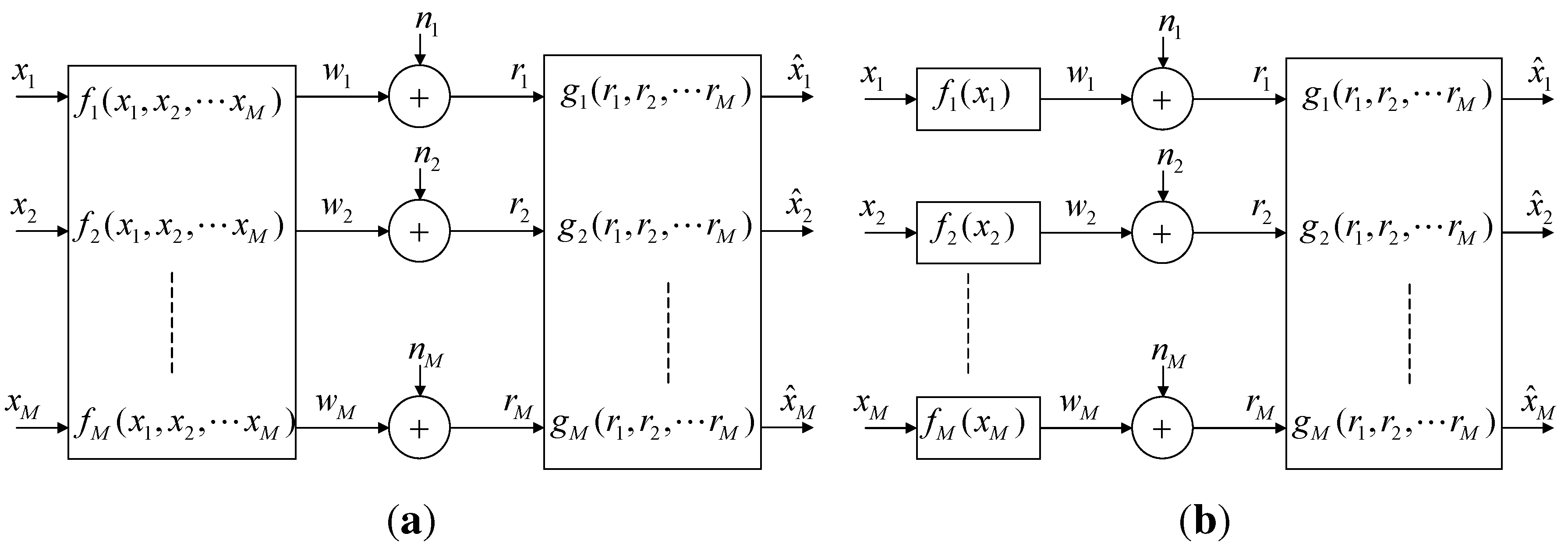
3. Optimal Linear Mappings

Optimal linear schemes are presented for both the distributed and the cooperative case.

3.1. Distributed Linear Mapping

At the encoder side, the observations are scaled at each sensor to satisfy the power constraint, P:
f i ( x i ) = P σ x 2 x i i = { 1 , 2 , . . . M }
At the decoder, we estimate each sensor observation utilizing all received channel outputs, r . For memoryless Gaussian sources, their MSE estimate can be expressed as linear combinations of the received channel symbols:
g i ( r ) = b i T r
b i are coefficients satisfying the Wiener-Hopf equations:
C r b i = C x i r , i = { 1 , 2 , . . . M }
where C r is the covariance matrix of the received vector, r , and C x i r is the cross-covariance matrix for x i and r . The average end-to-end distortion per source symbol is then given by D nc = σ x 2 - C r x i T b i , i = { 1 , 2 , . . . M } ( nc denotes “no cooperation”). All i terms are equal for the case treated in this paper, i.e., D 1 = D 2 = = D M = D n c . By inserting the relevant cross covariance matrices and the optimal coefficient vector, it is straight forward to show that:
D nc = σ x 2 - C r x i T b i = σ x 2 SNR ( 1 + ( M - 2 ) ρ x - ( M - 1 ) ρ x 2 ) + 1 SNR 2 ( 1 + ( M - 2 ) ρ x - ( M - 1 ) ρ x 2 ) + ( 2 + ( M - 2 ) ρ x ) SNR + 1

3.2. Cooperative Linear Mapping

When cooperation is possible, the sources can be decorrelated prior to transmission by a diagonalizing transform (which is a simple rotation operation when M = 2 ). The transmit power, M P , is then optimally allocated along the eigenvectors of C x . This scheme is also known as Block Pulse Amplitude Modulation (BPAM) [23]. The end-to-end distortion, D BPAM , is given by [16] (pp. 65–66) :
D BPAM = 1 2 σ n 2 i = 1 t λ i 2 t σ n 2 + M P + i = t + 1 M λ i
where t = min ( M , t ) and t is the smallest integer that satisfies:
σ n 2 λ t + 1 j = 1 t λ j - λ t + 1 M P
Case 1: The total power is allocated to all encoders, that is t = M , and so:
D BPAM ( 1 ) = 1 M σ n 2 i = 1 M λ i 2 M σ n 2 + M P = σ x 2 ( M - 1 ) ρ x + 1 + ( M - 1 ) 1 - ρ x 2 M 2 ( 1 + SNR )
Case 2: The total power is allocated only to the first encoder, that is t = t = 1 , and thus:
D BPAM ( 2 ) = 1 M σ n 2 λ 1 σ n 2 + M P + i = 2 M λ i = σ x 2 M ( M - 1 ) ρ x + 1 1 + M SNR + ( M - 1 ) ( 1 - ρ x )
To determine for which channel SNR Case 1 and Case 2 apply, assume that t = t = 1 . Then, Equation (14) becomes λ 1 - λ 2 / λ 2 M SNR . By inserting the eigenvalues, one can show that Case 2 is valid whenever:
SNR 1 M 1 + ( M - 1 ) ρ x 1 - ρ x - 1 = κ
The performance of any linear scheme for the network in Figure 1 is then, for SNR, 0 , bounded by:
D coop ( SNR ) = σ x 2 M ( M - 1 ) ρ x + 1 + ( M - 1 ) 1 - ρ x 2 M ( 1 + SNR ) , SNR > κ ( M - 1 ) ρ x + 1 1 + M SNR + ( M - 1 ) ( 1 - ρ x ) , SNR κ
Observe that the bound in Equation (5) results when inserting ρ x = 0 in both Equations (12) and (18).
The theoretical performance of both cooperative and distributed linear schemes are plotted for various M and ρ x in Figure 2, along with the OPTA curve for ρ x = 0 and OPTA c o o p .
Observe that when SNR is low, the cooperative and the distributed schemes coincide, regardless of M and ρ x . When SNR grows, the performance of the cooperative scheme remains parallel to that of OPTA coop , while the distributed scheme approaches the OPTA curve for ρ x = 0. The distributed linear scheme, therefore, fails to exploit correlation between the sources at a high SNR. The reason is that optimal power allocation is impossible in the distributed case, since decorrelation requires that the encoding function operate on all variables.
The conclusions we draw from the performances of the distributed linear scheme are somewhat different from the conclusions in [13]. There, the authors claimed that the distributed linear scheme (referred to as AF in their paper) performs close to optimal for all SNR and ρ x . As we can see from Figure 2b, this is not necessarily the case, especially at a high SNR. In addition, linear mappings are not necessarily suitable for all values of ρ x , since its gap to OPTA coop becomes substantial when ρ x gets close to one. Distributed linear coding, although simple, is basically meaningful to use at a relatively low SNR, since its performance converges to the ρ x = 0 case as SNR grows (except when ρ x = 1 ). When ρ x is close to one, a significant gain can be achieved by applying nonlinear mappings.

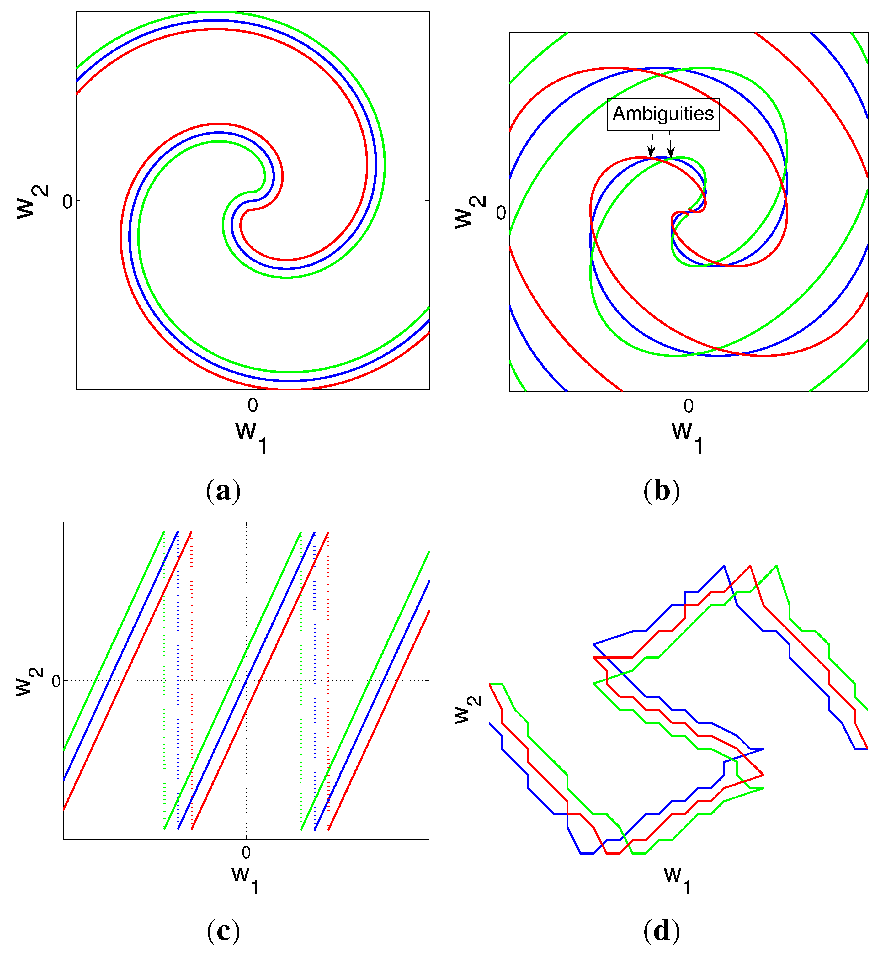
4. Nonlinear Mappings

The nonlinear mappings we apply for highly correlated sources are known as S-K mappings. We first review the basics of S-K mapping and illustrate how they apply directly in the distributed case when ρ x = 1 . We then generalize these mappings so that they apply to ρ x < 1 , but still close to one.

4.1. Special Case ρ x = 1

S-K mappings can be effectively designed for both bandwidth/dimension compression and expansion on point-to-point links [27,31]. Consider the dimension expansion of a single source (random variable): each source sample is mapped into M channel symbols or an M dimensional channel symbol. At the decoder side, the received noisy channel symbols are collected in M-tuples to jointly identify the single source sample. Such an expanding mapping, named 1:M mapping, can be realized by parametric curves residing in the channel space (as “continuous codebooks”), as shown in Figure 3 for the M = 2 and M = 3 case. The curves basically depict the one-dimensional source space as it appears in the channel space after being mapped through the S-K mapping. Noise will take the transmitted value away from the curve, and the task of the decoder is to identify the point on the curve that results in the smallest error. If we consider a Maximum Likelihood (ML) receiver, the decoded source symbol, x ^ m , is the point on the curve that is closest to the received vector. An ML decoder is therefore realized as a projection onto the curve [40]. One may also expand an M-dimensional source (M random variables) or M consecutive samples collected in a vector, into and N-dimensional channel symbol (where M < N ). Such an M:N expanding S-K mapping is realized as a hyper-surface residing in the channel space.
S-K mappings can be applied distributedly by encoding each variable by a unique function, f m ( x m ) :
f ( x ) = [ f 1 ( x 1 ) , f 2 ( x 2 ) , , f M ( x M ) ]
when ρ x = 1 , Equation (19) is really a dimension expanding S-K mapping, since x m = y m . That is, the same variable is coded and transmitted by all encoders. With the received signal, r ^ m = f m ( y ) + n m , the ML estimate of y is given by:
y ^ = arg min y f 1 ( y ) - r 1 2 + + f M ( y ) - r M 2
When M = 2 , a good choice of functions is the Archimedean spiral in Figure 3a, defined by [27]:
f 1 ( x 1 ) = ± ( Δ / π ) φ ( x 1 ) a cos ( φ ( x 1 ) ) , f 2 ( x 2 ) = ± ( Δ / π ) φ ( x 2 ) a sin ( φ ( x 2 ) )
where + is for positive source values (blue spiral), while − is for negative (red spiral). Δ reflects the distance between the blue and the red curves, φ ( · ) is a conveniently chosen mapping function and a determines if the distance between the spiral arms will diverge outwards ( a > 1 ), have constant distance ( a = 1 ) or collapse inwards ( a < 1 ). Similarly, the “Ball of Yarn” in Figure 3b is defined by [41]:
f 1 ( x 1 ) = ± ( Δ / π ) φ ( x 1 ) a cos φ ( x 1 ) / π sin ( φ ( x 1 ) ) , f 2 ( x 2 ) = ± ( Δ / π ) φ ( x 2 ) a sin φ ( x 2 / π ) sin ( φ ( x 2 ) ) , f 3 ( x 3 ) = ± ( Δ / π ) φ ( x 3 ) a cos ( φ ( x 3 ) ) .
when these transformed values are transmitted simultaneously on orthogonal channels, we get a Cartesian product resulting in the structures in Figure 3 (when ρ x =1). The performance of these mappings is shown in Figure 4 for a = 1 . 1 and several values of Δ, together with OPTA and distributed linear mappings. The optimal Δ is found in the same way as in [31], and a similar derivation is given in Section 4.5. Interpolation between optimal points are plotted for the M = 2 case, while a robustness plot (that is, Δ is fixed while the SNR varies; this shows how the mapping deteriorates as the channel SNR moves away from the optimal SNR) is plotted for the M = 3 case.
Figure 3. Shannon-Kotelnikov (S-K) mappings. The curves represent a scalar source mapped through f in the channel space. Positive source values reside on the blue curves, while negative reside on the red. (a) M = 2 : Archimedes spiral; (b) M = 3 : “Ball of Yarn”.
Entropy 15 02129 g003
Both the Archimedes spiral and the Ball of Yarn improve significantly over linear mappings. The distance to OPTA is quite large for the M = 3 case, but there is still a substantial gain of around 4–6 dB compared to the M = 2 case. A 1:3 mapping with better performance has been found in [42], but can only be applied with collaborative encoders. It has also been shown that S-K mappings can perform better at a low SNR using MMSE decoding [35].
One can get better insight into the design process of S-K mappings by understanding their distortion behavior. Analyzing nonlinear mappings in general is difficult, and in order to provide closed form expressions that can be interpreted further, we follow the method of Kotelnikov [18] (chapters 6–8) (see also [40] (chapter 8.2) and [38]) and divide the distortion into two main contributions: weak noise distortion, denoted by ε ¯ w n 2 , and anomalous distortion, denoted by ε ¯ t h 2 .
Figure 4. Performance of S-K mappings when M = 2 , 3 for several values of Δ.
Entropy 15 02129 g004
Weak noise distortion results from channel noise being mapped through the nonlinear mapping at the receiver and refers to the case when the error in the reconstruction varies gradually with the magnitude of the channel noise (non-anomalous errors). For a curve, f , weak noise distortion is quantified by [18,31]:
ε ¯ w n 2 = σ n 2 D 1 f ( y ) 2 p y ( y ) d y
where D is the domain of the source and p y ( y ) its pdf (we use y here, since x 1 = = x M = y , when ρ x = 1 ). f ( y ) is the length of the tangent vector of the curve at the point, y. The Equation (23) says that the more the source space (y) is stretched by the S-K mapping, f , at the encoder side (think about stretching of the real line like a rubber band or a nonlinear amplification), the more the channel noise will be suppressed (attenuated) when mapped through the inverse mapping at the receiver. If the curve should be stretched a significant amount without violating a channel power constraint, a nonlinear mapping that “twists” the curve into the constrained region is needed, as illustrated in Figure 5a.
Still, the curve must have finite length (it cannot be stretched indefinitely), since, otherwise, anomalies, also called threshold effects [17,43], will occur. Anomalies can be understood as follows: Consider the 1:2 mapping in Figure 5b. When the distance between the spiral arms (Δ) becomes too small, for a given noise variance, σ n 2 , the transmitted value, f ( y 0 ) , may be detected as f ( y + ) on another fold of the curve at the receiver. The resulting distortion when averaging over all such incidents is what we have named anomalous distortion (see, e.g., [31] or Section 4.5 for more details). Since anomalous distortion depend on the structure of the chosen mapping, we only state that the pdf needed to calculate the probability for such errors here and give a specific example on how to calculate anomalous distortion for the Archimedes spiral in Section 4.5. The pdf of the norm, ϱ = n ˜ , for an N-dimensional vector, n ˜ , with i.i.d. Gaussian components, is given in [44] (p. 237):
p ϱ ( ϱ ) = 2 ( N 2 ) N 2 ϱ N - 1 Γ ( N 2 ) σ n N e - N 2 ϱ 2 σ n 2 , N 1
Note that if f ( y ) is chosen, so that only noise vectors perpendicular to it, n , lead to anomalous errors (like the spiral in Figure 5), then N = M - 1 . Anomalous errors happen in general if the norm, ϱ, gets larger than a specific value. For instance, for the Archimedes spiral, the probability for anomalies are give by P r { ϱ Δ / 2 } when a = 1 (around the optimal Δ).
Figure 5. 1:2 S-K mappings. (a) Linear and nonlinear mappings; (b) when spiral arms come too close, noise may take the transmitted vector, f ( y 0 ) , closer to another fold of the curve, leading to large decoding errors.
Entropy 15 02129 g005
There is a tradeoff between the two distortion effects, which results in an optimal curve length for a given channel SNR (this corresponds to an optimal Δ for the Archimedes spiral and Ball of Yarn). The two distortion effects can be seen for the M = 3 case in Figure 4, where ε ¯ w n 2 dominates above the optimal point and ε ¯ t h 2 dominates below. Note specifically that ε ¯ w n 2 has the same slope as a linear mapping, which results from the fact that a linear approximation to any continuous (one-to-one) nonlinear mapping is valid at each point if σ n is sufficiently small.

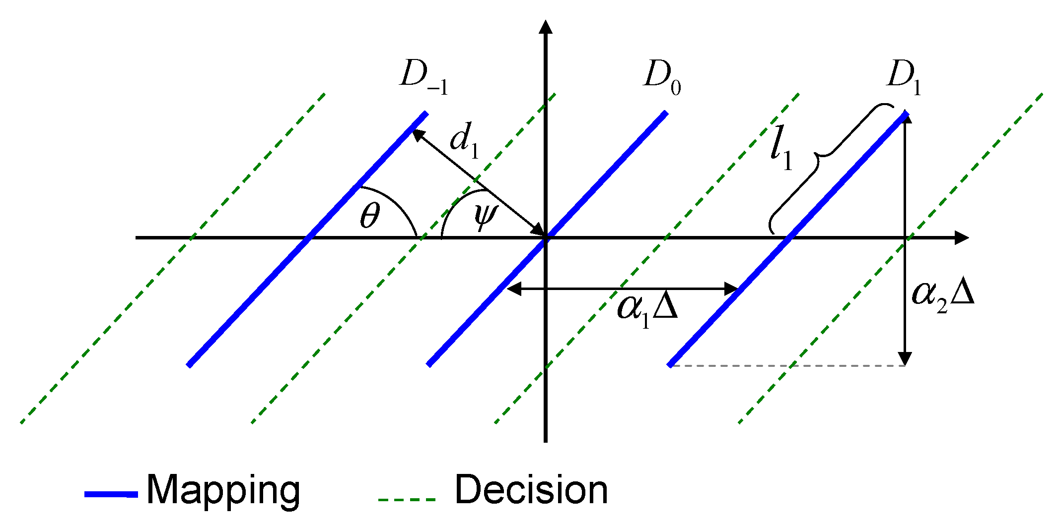
4.2. Nonlinear Mappings for ρ x < 1

The situation becomes more complicated when ρ x < 1 . Since λ 1 > λ 2 = λ 3 =⋯= λ M , it is straight forward to deduce from the reverse water-filling principle [45] that only the largest eigenvalue (here λ 1 ) should be represented when SNR is below a certain threshold (for instance, for the bound in Equation (5); this threshold is given by SNR = ( 1 + ( M - 1 ) ρ x ) / ( 1 - ρ x ) M - 1 ). That is, only transmission and decoding of y should be considered below a certain SNR. Above this threshold, one should consider all eigenvalues, i.e., transmit and decode all individual observations.
One can get an idea on how specific mappings should be constructed when M = 2 from the distributed quantizer (DQ) scheme in [9]. There, each node quantizes its source using a scalar quantizer.Figure 6a and Figure 6b show the DQ centroids plotted in pairs in the two-dimensional channel space for ρ x = 0 . 95 and 0 . 99 .
Figure 6. Channel space structures when M = 2 and ρ x < 1 . (a) 5 bit distributed quantizer (DQ), ρ x = 0 . 95 ; (b) 5 bit DQ, ρ x = 0 . 99 ; (c) sawtooth mapping, ρ x = 0 . 99 ; (d) Archimedes spiral, ρ x = 0 . 999 .
Entropy 15 02129 g006
Observe that the DQ centroids in Figure 6b lie on a thin spiral-like surface strip that is “twisted” into the channel space. One possible way to construct a continuous mapping is to use the parametric curves introduced for the ρ x = 1 case as they are, i.e., use Equations (21) and (22) directly. Inspired from Figure 6b, we choose to apply the Archimedes spiral in Equation (21), shown in Figure 6c, when ρ x = 0 . 999 . Compared to Figure 3a, the spiral is now “widened” into a thin surface strip.
We propose a mapping for collaborative encoders for the M = 2 case to provide insight into what benefits collaboration may bring. To simplify, we make a change of variables from x 1 , x 2 to the independent variables, y a = ( x 1 + x 2 ) / 2 and z a = ( x 2 - x 1 ) / 2 . y a is aligned with the first eigenvector of C x , while z a is aligned with the second eigenvector. One possible generalization of the spiral in Equation (21) is:
f ( y a , z a ) = h ( y a ) + N ( y a ) α z z a
where h ( y a ) is the Archimedes spiral in Equation (21) and N ( y a ) is the unit normal vector to the spiral at the point, h ( y a ) . One can use Appendix A to show that the components of N ( y a ) are:
N 1 ( y a ) = - φ ( y a ) cos ( φ ( y a ) ) + sin ( φ ( y a ) ) 1 + φ 2 ( y a ) , N 2 ( y a ) = cos ( φ ( y a ) ) - φ ( y a ) sin ( φ ( y a ) ) 1 + φ 2 ( y a )
A similar generalization can be applied to other parametric curves, h ( y ) , for any M.
To provide geometrical insight into how two correlated variables are transformed by Equations (25) and (21), we show how they transform the three parallel lines, x 2 = x 1 - κ (red), x 2 = x 1 (blue) and x 2 = x 1 + κ (green), in Figure 7a and Figure 7b, respectively.
The generalized spiral in Equation (25) represents both common information (the blue curve) and the individual contributions from both sources uniquely. The distributed mapping in Figure 7b represents common information well, but ambiguities will distort the individual contributions in certain intervals: The green curve in Figure 7b results by inserting x 2 = x 1 + κ in Equation (21), which is a “deformed” spiral lying inside an ellipse with the major axis aligned along the function, w 2 = w 1 . The red spiral, on the other hand, is lying inside an ellipse with the major axis aligned along w 2 = - w 1 . These spirals are therefore destined to cross at certain points. Ambiguities can also be observed for similar mappings found in the literature. One example is the DQ in Figure 6b, as illustrated in Figure 7d. Whether continuous mappings that avoid ambiguities can be found when the encoders operate on only one variable is uncertain. Further research is needed in order to conclude.
An alternative mapping that avoids ambiguities in the distributed case is the piecewise continuous sawtooth mapping proposed in [8], depicted in Figure 6d. Although this mapping was proposed for transmission of noisy observations of a single random variable, it is applicable for the coding of several correlated variables by a slight change in the decoder. The encoders for the M = 2 case are given by:
f 1 ( x 1 ) = α 1 x 1 , f 2 ( x 2 ) = α 2 x 2 - Δ x 2 Δ ,
where Δ determines the period of the sawtooth function, f 2 , and α 1 , α 2 makes it possible to control the power for each encoder separately. We use this mapping as an example for M = 2 . It can easily be extended to both arbitrary M, as shown in [8] and blocks of samples (code length beyond one), as shown in [10], which makes it a good choice of mapping. From Figure 7c, one can observe that ambiguities are avoided.
Figure 7. How the three lines, x 2 = x 1 - κ (red), x 2 = x 1 (blue) and x 2 = x 1 + κ (green), are mapped by selected nonlinear mappings. (a) Collaborative mapping in Equation (25); (b) distributed mapping in Equation (21); (c) sawtooth mapping in Equation (27); (d) DQ from Figure 6b.
Entropy 15 02129 g007
To determine the reconstruction, x ^ m , m = 1 , , M , we first decode y then z m . y is found by projecting the received vector onto the closest point on the curve representing common information, f ( y ) . f ( y ) corresponds to the blue curves shown in Figure 7a and Figure 7b when M = 2 . The ML detector for y is therefore given in Equation (20). Given y ^ , the individual contributions, z m , can be found by mapping values of z = [ z 1 , , z M ] within an M-ball of a certain radius, ϱ, through the encoding functions, f , then choose the z that results in the smallest distance to the received vector. For the collaborative case:
z ^ = arg min z 1 , , z M : z ϱ f 1 ( y ^ + z 1 , , y ^ + z M ) - r 1 2 + + f M ( y ^ + z 1 , , y ^ + z M ) - r M 2
whereas for the distributed case:
z ^ = arg min z 1 , , z M : z ϱ f 1 ( y ^ + z 1 ) - r 1 2 + + f M ( y ^ + z M ) - r M 2
Note that ϱ decreases with increasing ρ x , making the search for z simpler. If ϱ is chosen as too large, then anomalous errors will result. The reconstruction is finally given by x ^ m = y ^ + z ^ m . Note that in order to achieve the best possible result at low SNR, one should use MMSE decoding. Since only y is reconstructed at low SNR, a similar approach to that in [35] for dimension expanding S-K mappings may be used. We leave out this issue and refer to [35] as one possible way to achieve better performance.
In the following sections, distortion and power expressions are given. These expressions will facilitate analysis and optimization of S-K mappings for the network under consideration.

4.3. Power and Distortion Formulation: Collaborative Encoders

To calculate power and distortion, we apply and generalize selected results from [8,31,32,38]. For both cases, the formulation of the problem will depend on whether only common information or both common information, as well as individual contributions should be reconstructed at the receiver. Details in some derivations are omitted, since they require substantial space.

4.3.1. Reconstruction of Common Information

When the encoders collaborate, one may drop all individual contributions, z m , prior to transmission by averaging over all variables, y a = ( x 1 + x 2 + + x M ) / M , and so, y a N ( 0 , σ y a 2 ) with σ y a 2 = E { y a 2 } = σ x 2 1 + ( M - 1 ) ρ x / M . y a is then encoded by a parametric curve, f ( y a ) = [ f 1 ( y a ) , f 2 ( y a ) , , f M ( y a ) ] , and therefore, the same distortion contributions as for the ρ x = 1 case in Section 4.1 apply. That is, Equation (23) quantifies weak noise distortion by exchanging y with y a and the pdf, p y ( y ) , with p y a ( y a ) , and the probability for anomalous errors can be found from Equation (24).
We also get a distortion contribution from excluding z m . This contribution is reflected in the fact that the eigenvalues, λ m , m = 2 , , M , are not represented. The distortion is given by the sum of these eigenvalues divided over all M sources:
ε ¯ l 2 = 1 M m = 2 M λ m = σ x 2 ( M - 1 ) ( 1 - ρ x ) M
The power per source symbol is given by [31]:
P a = 1 M f ( y a ) 2 p y a ( y a ) d y a

4.3.2. Reconstruction of Common Information and Individual Contributions

With f ( x ) = [ f 1 ( x ) , f 2 ( x ) , , f M ( x ) ] , the power per source symbol becomes:
P a = 1 M M - fold f ( x ) 2 p x ( x ) d x
Since all eigenvalues are now represented, the distortion in Equation (30) will disappear. The weak noise and anomalous distortion need to be modified.
Weak Noise Distortion: Although we have M variables communicated on M channels, expansion of x by an S-K mapping is possible when ρ x is close to one (for similar reasons as in Section 4.1). A similar analysis as that in [32,38] for M:N dimension expanding S-K mappings can therefore be applied.
We now have a thin M-dimensional hyper-surface strip of dimension M that is twisted and bent into the M-dimensional channel space (like the structure in Figure 7a). That is, a subset of R M is mapped into R M . An important fact is that weak noise distortion is defined intrinsically [32,38], i.e., it is defined only on the M-dimensional surface representing the S-K mapping, independent of any surrounding coordinate system. One can therefore calculate weak noise distortion here in the same way as in [38]. For brevity, we only state the result and explain the essentials of the given expression. The reader may consult [38] for details in the derivation. We have:
ε ¯ w n 2 = σ n 2 M D M - fold i = 1 M 1 g i i ( x ) p x ( x ) d x ,
with p x ( x ) given in Equation (1) and D , the relevant domain of the source space. g i i , i = 1 , , M , denote the diagonal components of the so-called metric tensor, described in Appendix B (an intrinsic feature of the surface, f ), which corresponds to the squared norm of the tangent vectors along f ( x i ) , i = 1 , , M . These components quantify the nonlinear “magnification” done by f on the source vector, x . Note that Equation (33) is a generalization of Equation (23) and basically says that the more the source, x , is stretched/magnified by f (in all M directions) at the encoder, the more suppressed the channel noise will become when mapped through the inverse mapping at the receiver. (Note that for Equation (33) to be valid, all off-diagonal components g i j = 0 ; this is the case for all mappings treated in this paper.)
Anomalous distortion: Anomalies now refer to the confusion of x 1 , , x M with the vector, x ˜ 1 , , x ˜ M , on another fold of the mapping. For instance, in Figure 7a, vectors between the blue and green spirals may get exchanged with values along the green spiral on another fold. We only derive the pdf needed to calculate the probability for anomalous errors here and give a specific example on how to calculate anomalous distortion in Section 4.5.
The probability for anomalies now depends on both the noise, n and z , since the mapping “widens” with the magnitude of z m . Let y 0 denote an M-dimensional vector with all components equal to y 0 . To be able to calculate the pdf of z after the nonlinear mapping, f ( x 1 , , x M ) , given that y = y 0 , we have to assume that ρ x is close enough to one ( z m small) to consider the linear approximation:
f ( y 0 + z ) f ( y 0 ) + J ( y 0 ) z
J ( y 0 ) is the Jacobian of f ( x 1 , , x M ) , evaluated at x m = y 0 , m = 1 , , M (see Appendix B). The variance per dimension of the transformed vector, z T = J ( y 0 ) z , is then given by σ z T 2 ( y 0 ) = ( 1 / M ) E ( J ( y 0 ) z ) T ( J ( y 0 ) z ) . By assuming that the off-diagonal components of the metric tensor of f is g i j = 0 , the same arguments as in [38] lead to:
σ z T 2 ( y ) = 1 M E z T T z T = σ z 2 M i = 1 M g i i ( y )
The g i i ( y ) ’s reflects the magnification of z given y and are given by:
g i i ( y ) = f x i , f x i | x i = y
Let z ˜ T and n ˜ denote the N-dimensional sub-vectors of z T and n at f ( y 0 ) that point in the direction of the closest point on another fold of f (like n in Figure 5a). The pdf of the sum, z ˜ T + n ˜ , is given by a convolution [46] p z ˜ T ( z ˜ T , y ) p n ˜ ( n ˜ ) . Since both p z ˜ T and p n ˜ are i.i.d. Gaussians, the convolution is also Gaussian [46], with variance σ z T , n 2 ( y ) = σ z T ( y ) 2 + σ n 2 . From Equation (24), with ϱ a n = z ˜ T + n ˜ , we get:
p ϱ a n ( ϱ a n , y ) = 2 ( N 2 ) N 2 ϱ a n N - 1 Γ ( N 2 ) σ z T , n ( y ) N e - N 2 ϱ a n 2 σ z T , n ( y ) 2 , N 1

4.4. Distributed Encoders: ρ x < 1

Since each encoder operates on only one variable, it is not possible to diagonalize or take averages, implying that one cannot remove z m prior to transmission. The average power is therefore given by the same expression, whether transmission of common information or both common information and individual contributions are considered:
P a = 1 M m = 1 M P m = 1 M m = 1 M f m 2 ( x m ) p x m ( x m ) d x m

4.4.1. Reconstruction of Common Information

The distortion from not representing the eigenvalues, λ 2 , , λ M , is again given by Equation (30).
Weak noise distortion: The individual contributions, z , will now represent noise that corrupts the value of y. If ρ x is close to one, then the variance of z m will be small enough to consider the linear approximation, f ( y + z m ) f ( y ) + z m f ( y ) . We are then in the same situation as in [8], and the distortion can be derived in the same way. The result is (consult [8] for details):
ε ¯ w n 2 = σ z 2 m = 1 M f i ( y ) 4 f ( y ) 4 + σ n 2 f ( y ) 2 p y ( y ) d y
The first term accounts for distortion due to z m , whereas the last term accounts for distortion due to channel noise and is the same as in Equation (23). It was shown in [8] that the first term in Equation (39) is minimized by a linear mapping. On the other hand, a linear mapping is, in most cases, sub-optimal when it comes to suppressing channel noise, i.e., minimizing the second term in Equation (39). There is, therefore, a tradeoff between lowering distortion, due to z and channel noise.
Anomalous distortion: Since z m cannot be removed prior to transmission, the pdf needed to calculate probability for anomalous errors is basically the same as in Equation (37), except that the metric tensor is different. The diagonal components of the metric tensor is now:
g i i ( y ) = f x i , f x i | x i = y = d f i d x i , d f i d x i | x i = y

4.4.2. Reconstruction of Common Information and Individual Contributions
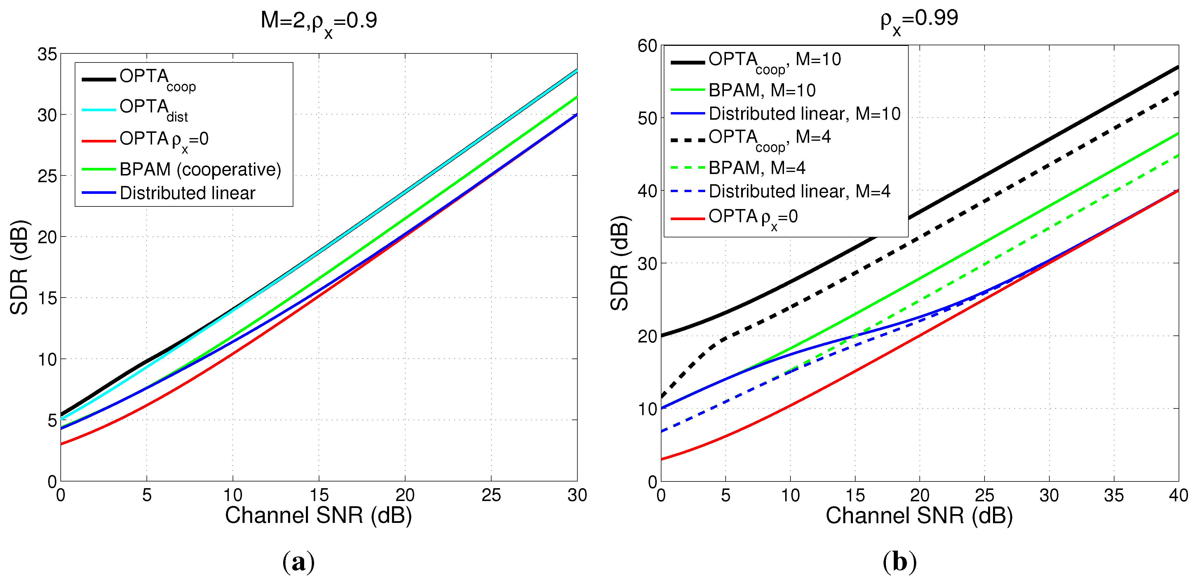
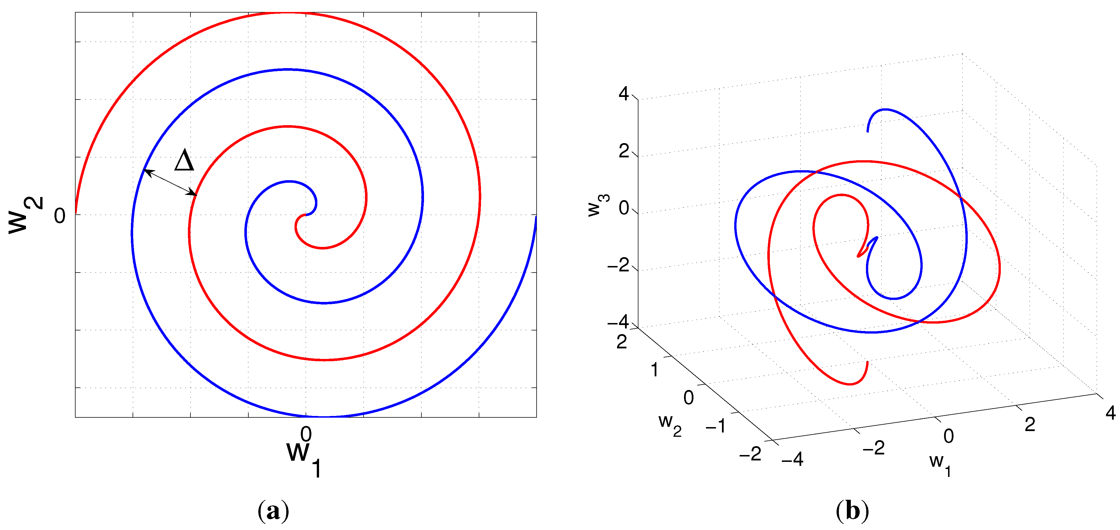
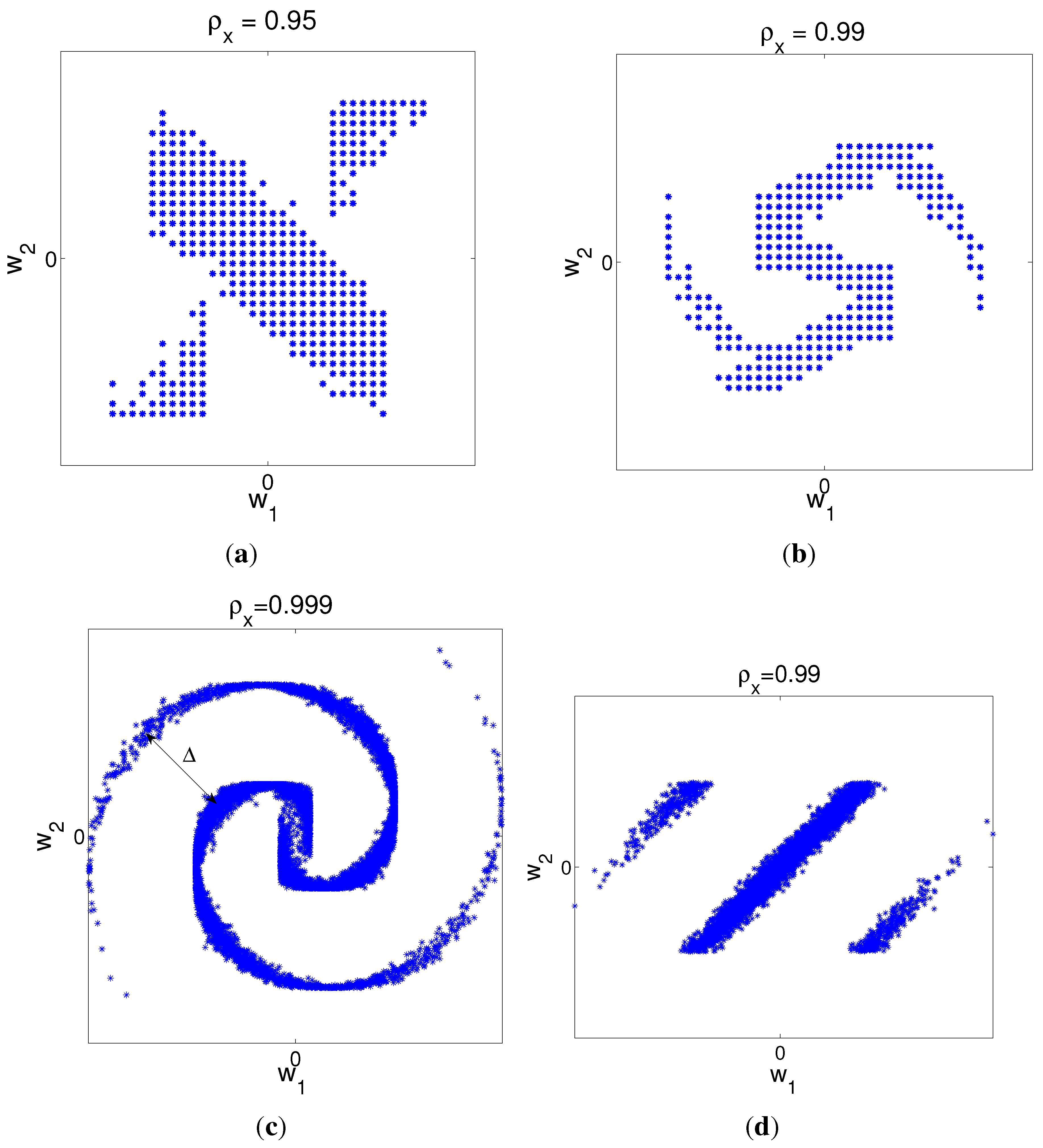
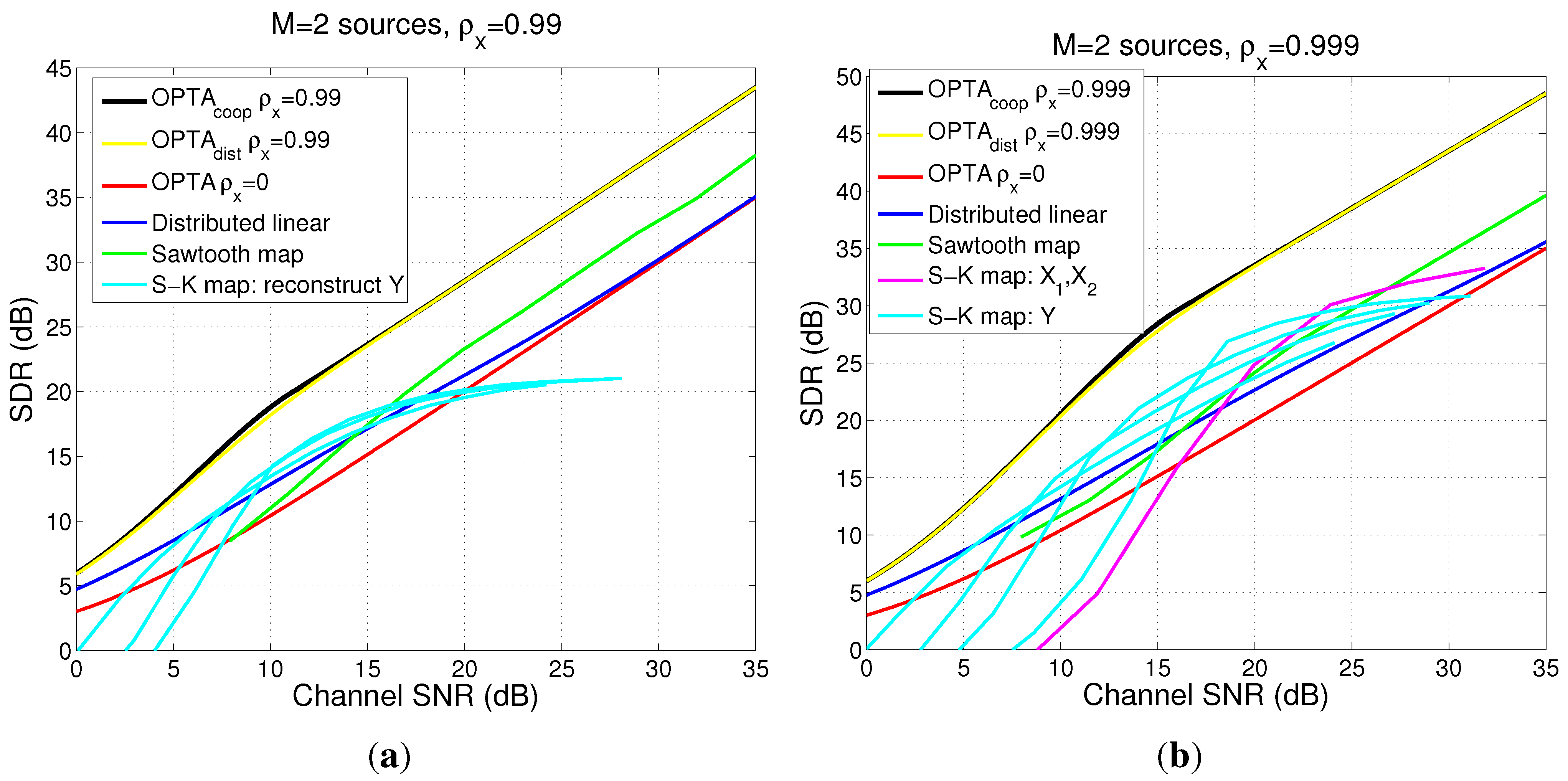
The power is given by Equation (38), and the pdf needed to calculate probability for anomalous errors is given by Equation (37), with the g i i ’s in Equation (40).
The weak noise distortion must be reformulated, and a distortion contribution, due to the ambiguities mentioned earlier (shown in Figure 7b), must be added.
Weak noise distortion: Weak noise distortion now refers to distortion in the areas without ambiguities, that is, where each source vector has a unique representation after being mapped through f . Since g i i ( x ) = g i i ( x i ) = f i ( x i ) 2 [see Equation (40)] is a function of only one variable, Equation (33) is reduced to:
ε ¯ w n 2 = σ n 2 M D M - fold i = 1 M 1 f i ( x i ) 2 p x ( x ) d x = σ n 2 M i = 1 M 1 f i ( x i ) 2 p x i ( x i ) d x i
The integral domain, D , is over all x i for a mapping that avoids ambiguities (like the sawtooth mapping) and over the domain without ambiguities otherwise.
Distortion due to ambiguities: Picture the M = 2 case. For continuous mappings, like the spiral shown in Figure 7b, remote source values, represented by the green and red lines, may cross in certain intervals, leading to ambiguities at the decoder. Ambiguities will make the decoder interchange values along the minor axis (or minor axes for general M). When the green and red lines cross, positive and negative values may be interchanged, which lead to a large error in the decoded value. If a continuous mapping is to be applied, it is better to only decode common information in the areas where ambiguities are prominent (for instance, in the interval between the arrows in Figure 7b).
Assume that ambiguities happen in the intervals [ y i , y i + 1 ] and that there are K such intervals in total. If we decode only common information in these intervals, the distortion is quantified by:
ε ¯ a m 2 = i = 1 K y i y i + 1 ε ¯ l 2 + σ z 2 m = 1 M f i ( y ) 4 f ( y ) 4 + σ n 2 f ( y ) 2 p y ( y ) d y
while Equation (41) quantifies distortion outside these intervals. ε ¯ l 2 is given by Equation (30) and takes into account the distortion from only representing common information. The second term takes into account the distortion due to z m , and the last term is distortion due to channel noise. To determine the values of y i and y i + 1 , the relevant intersection points must be found (for instance, where the red and green spirals cross the blue spiral in Figure 7b).

4.5. Examples for the ρ x < 1 Case When M = 2

In this section, the mappings in Equations (25), (21) and (27) will be optimized using the power and distortion analysis presented in the preceding sections, then simulations of the optimized mappings are given.
First a suitable function, φ must be chosen for the spiral in Equation (21). In [31], it was argued why choosing φ as the inverse curve length is convenient. For the spiral, the curve length function is similar to a quadratic function. Since it is unknown for the problem at hand which function is optimal, we choose the inverse of φ to be the polynomial φ - 1 = ( θ ) = Δ ( a θ 2 + b θ ) , and so:
φ ( x m ) = ± 1 2 a b 2 + 4 a α | x m | Δ - b 2 a
a and b are coefficients that will be optimized, α is an amplification factor and ± reflects the sign of x m .

4.5.1. Power and Distortion Calculation for Collaborating Encoders

The spiral in Equation (21) is applied when only common information is transmitted, and the generalized spiral in Equation (25) is applied when individual contributions, z 1 and z 2 , are included.
Reconstruction of common information: Here, only the average, y a = ( x 1 + x 2 ) / 2 , is transmitted.
To calculate the power, the norm, f ( y a ) , is needed. By sin 2 ( x ) + cos 2 ( x ) = 1 , it is easy to show that:
f ( y a ) 2 = Δ π 2 φ 2 ( y a )
The power is found by inserting Equation (44) in Equation (31) with M = 2 .
Since z 1 and z 2 are not transmitted, the distortion, ε ¯ l 2 = σ x 2 ( 1 - ρ x ) / 2 , results [insert M = 2 in Equation (30)].
Weak noise distortion is found by inserting M = 2 in Equation (23), exchanging y with y a and p y ( y ) with p y a ( y a ) . By again using sin 2 ( x ) + cos 2 ( x ) = 1 , one can show that:
f ( y a ) 2 = Δ π φ ( y a ) 2 1 + φ 2 ( y a )
A good approximation to anomalous distortion must be found: With only y a transmitted, we only need to consider the blue spiral in Figure 7a. Then, the same method as in [31] applies, which we restate here for clarity. Figure 8 illustrates how to determine anomalous errors approximately.
Figure 8. Illustration on how to approximately calculate anomalous errors when only common information is to be reconstructed.
Entropy 15 02129 g008
The green curve depicts the noise pdf for a given y a . Since anomalies are mainly caused by the one-dimensional noise component perpendicular to the spiral (at least, close to the optimal operation point), denoted n , the wanted pdf is found by inserting N = 1 in Equation (24). The result is the Gaussian distribution, n N ( 0 , σ n 2 ) , denoted by p n ( n ) . When n crosses the black dotted curve in Figure 8, anomalous errors result. The probability of anomalous errors, given that y a was transmitted, is therefore:
P t h = P r { n > Δ / 2 } = Δ / 2 p n ( n ) d n = 1 2 1 - erf Δ 2 2 σ n
To determine the errors magnitude, assume first that f ( y a ) is moved outwards and exchanged with the nearest point on the neighboring spiral arm. That is, f ( y a ) is detected as f + = f ( y a ) + Δ . By converting to polar coordinates, we get - Δ φ ( y ^ + ) / π = Δ φ ( y a ) / π + Δ . By solving this with respect to y + ^ and using the same argument for noise moving the transmitted vector inwards to f - , we get:
y ^ ± = - φ - 1 ( φ ( y a ) ± π )
An approximation of the anomalous distortion is therefore given by:
ε ¯ a n 2 = 2 P t h 0 ( y a - y ^ + ) 2 + ( y a - y ^ - ) 2 p y a ( y a ) d y a
This expression is accurate around the mappings’ optimal SNR, whereas it may differ if the SNR drops far below optimum. It serves well in order to determine the optimal parameters.
Reconstruction of individual contributions: The decoder in Equation (28) is simplified with the generalized spiral in Equation (25), since we only need to search over one variable, z a = ( x 2 - x 1 ) / 2 (instead of z 1 and z 2 ).
To calculate the power, f ( y a , z a ) must be determined. Since:
f ( y a , z a ) 2 = m = 1 2 h m ( y a ) + α z N m ( y a ) z a 2
and by using the fact that E { h m ( y a ) z a } = 0 , N 1 2 ( y a ) + N 2 2 ( y a ) = 1 (unit normal vector) and h 1 2 ( y a ) + h 2 2 ( y a ) = φ 2 ( y a ) , Equation (32) is reduced to:
P a = 1 2 Δ 2 π 2 φ 2 ( y a ) p y a ( y a ) d y a + α z 2 σ z a 2
where σ z a 2 = E { z a 2 } = σ x 2 ( 1 - ρ x ) / 2 .
Weak noise distortion is found from Equation (33) by inserting M = 2 . The g i i ’s must be determined. Since f ( y a , z a ) / z a = α z [ N 1 ( y a ) , N 2 ( y a ) ] T and N 1 2 ( y a ) + N 2 2 ( y a ) = 1 :
g 22 ( y a , z a ) = f ( y a , z a ) z a , f ( y a , z a ) z a = α z 2
For g 11 :
g 11 ( y a , z a ) = f ( y a , z a ) y a , f ( y a , z a ) y a = m = 1 2 h m ( y a ) y a + α z z a N m ( y a ) y a 2
By using the fact that E { f ( y a ) z a } = 0 (for any measurable function f) and Equation (45), one can show that:
ε ¯ w n 2 = σ n 2 π 2 Δ 2 1 φ ( y a ) 2 1 + φ 2 ( y a ) d y a + 1 α z 2
To calculate anomalous distortion, a similar procedure as the one that led to Equation (48) can be applied. The fact that the spiral in Figure 8 “widens” due to z a has to be taken into account. With the mapping in Equation (25), y a moves along the spiral, h ( y a ) , while z a moves normal to it. Therefore, only g 22 affects the probability for anomalies (since it magnifies z a ). The relevant pdf is found by inserting N = 1 in Equation (37) with σ z T , n 2 = g 22 σ z a 2 + σ n 2 = α z 2 σ x 2 ( 1 - ρ x ) / 2 + σ n 2 , which is a Gaussian distribution. With the construction in Equation (25), the error probability will be the same for any given y a . With κ ( y ) = α z 2 σ x 2 ( 1 - ρ x ) + 2 σ n 2 , then:
P t h = Δ / 2 p ϱ a n ( ϱ a n ) d ϱ a n = 1 2 1 - erf Δ 2 κ ( y )
In Equation (48), the magnitude of anomalous errors was calculated by assuming that points on the blue solid-line spiral in Figure 8 were exchanged with points on the dashed blue spiral (or the other way around). Here, as can be seen from Figure 7a, either values lying between the blue and green spirals will get exchanged with points on the green spiral on another fold, or values between the red and blue spiral get exchanged with values on the red spiral on another fold. This makes the error somewhat smaller than in Equation (48). The difference in the error for these two cases is small when ρ x is close to one. To simplify calculations, we therefore choose to use the same error here as in Equation (48), which gives an upper bound on the error. The anomalous distortion is therefore bounded by Equation (48) with P t h given in Equation (54).
Optimization and simulation: A constrained optimization problem must be solved in order to determine the optimal free parameters, α, Δ, a and b for the spiral and α, α z , Δ, a and b for the generalized spiral. All parameters are functions of the channel SNR. With P m a x , the maximum allowed power per encoder output, and D t , the sum of all distortion contributions for the relevant case:
min a , b , α , α z , Δ : P a < P m a x D t
All parameters must also be positive. The problem must be solved numerically.
The S-K mappings are simulated using the optimized parameters. Figure 9 shows the performance for cooperative S-K mappings compared to OPTA c o o p and BPAM when ρ x = 0 . 99 and 0 . 999 .
The nonlinear S-K mappings outperform BPAM for most SNR, most significantly so when ρ x = 0 . 999 . Robustness plots are shown for S-K mappings for several sets of optimal parameters. The cyan curves show the performance when only common information is reconstructed. The performance levels off and becomes inferior to BPAM at about a 22 dB channel SNR when ρ x = 0 . 99 and 29 dB when ρ x = 0 . 999 . The reason is that the distortion term, ε ¯ l 2 = σ x 2 ( 1 - ρ x ) / 2 , results from not transmitting z a . The spiral is also quite robust against variations in SNR. With the generalized spiral in Equation (25), shown by the green curve, the performance does not level off at large SNR, and it does, in fact, maintain a constant gap to OPTA c o o p , as SNR increases without changing α, α z , Δ, a and b. This can be explained geometrically: as long as only y a should be transmitted, one can let the distance between the spiral arms, Δ, drop as SNR increases and, thereby, increase the curve length of f , resulting in a larger magnification of y a . This leads to a unique optimal SNR for each value of Δ, as shown by the cyan curves. When both y a and z p are transmitted, the spiral widens, and there must therefore be a lower bound on Δ = Δ m i n , if anomalous errors should be avoided. Then, with the right choice of Δ m i n , weak noise distortion will be the only contributions to total distortion when the SNR gets high enough. As mentioned earlier, weak noise distortion has the same slope as the distortion of (linear) BPAM. This effect is also reflected in OPTA c o o p , since it has the same slope as BPAM when SNR gets high enough.
Figure 9. Performance of cooperative S-K mappings (simulated) and Block Pulse Amplitude Modulation (BPAM) for M = 2 sources when (a) ρ x = 0 . 99 ; (b) ρ x = 0 . 999 .
Entropy 15 02129 g009

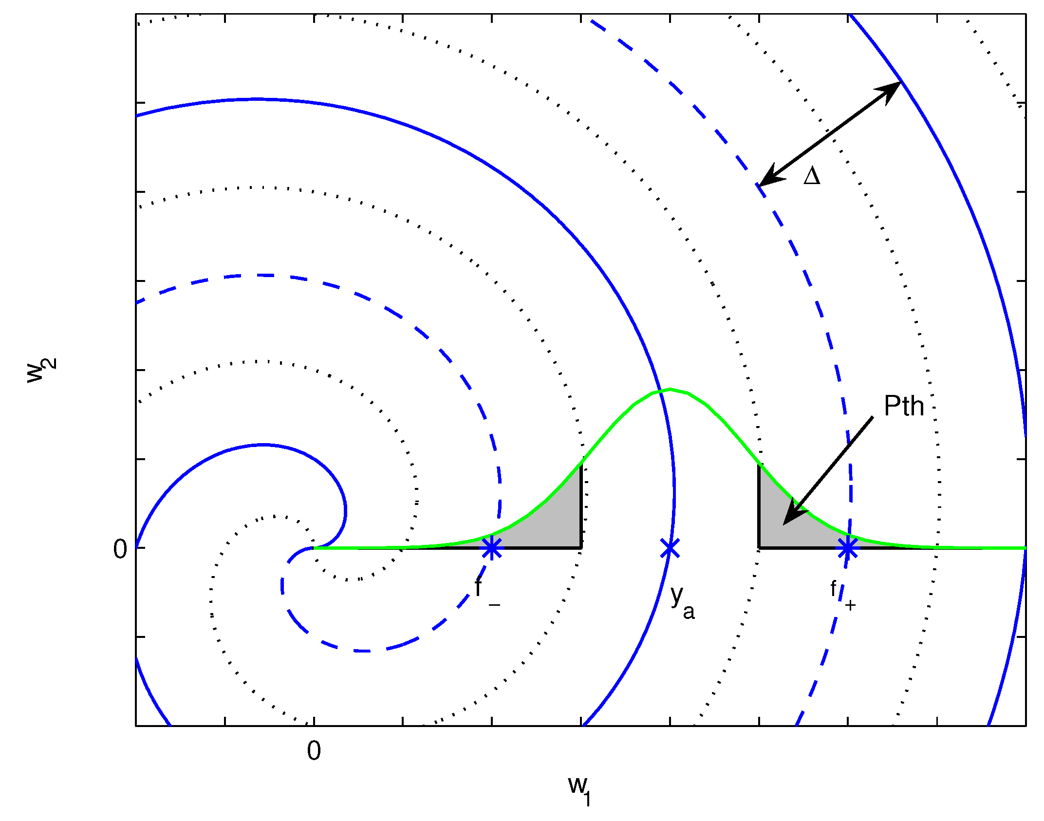
4.5.2. Power and Distortion Calculation for Distributed Encoders

Diagonalizing transforms cannot be applied in this case. Some derivations and expressions are, therefore, long and complicated, and some have to be found numerically. For brevity, we avoid stating some of the power and distortion expressions and just mention how they can be found numerically.
Reconstruction of common information: The output power is found by inserting the Equation (21) with a = 1 and M = 2 in Equation (38) and doing the integration numerically. Since decoding of z 1 and z 2 are not considered, we get the distortion term, ε ¯ l 2 = σ x 2 ( 1 - ρ x ) / 2 . Weak noise distortion is found by inserting M = 2 and the derivatives of Equation (21) evaluated at y in Equation (39), then doing the integration numerically.
Anomalous distortion can be calculated in a similar way as in Equation (48), but we have to take into account that z 1 and z 2 cannot be removed prior to transmission. From Figure 7b, one can observe that P t h depends on y (where we are on the blue spiral) and must be moved inside the integral in Equation (48) (we now integrate over y, not y a ). P t h ( y ) is found by changing κ in Equation (54) to κ ( y ) = σ x 2 ( 1 - ρ x ) ( g 11 ( y ) + g 22 ( y ) ) + 2 σ n 2 . The g i i ’s are found from Equation (40), i.e., the partial derivatives of Equation (21) w.r.t., x 1 and x 2 , evaluated at y.
Reconstruction of individual contributions: Two examples are considered: (1) spiral mapping and (2) sawtooth mapping.
(1) Spiral mapping: We may use the same power and anomalous distortion as we did when considering common information, since the encoders are the same [given by Equation (21)].
To reduce errors from ambiguities, we choose to decode only common information (values along the blue curve in Figure 7b) whenever ambiguities are present. The distortion is then given by Equation (42) with M = 2 . One can numerically determine where the green and red spirals cross the blue spiral in Figure 7b in order to find the intervals, [ y i , y i + 1 ] .
The calculation of weak noise distortion is complicated by two reasons: First, g i i ( x i ) = f ( x i ) 2 for the functions in Equation (21) contains zeros, implying that 1 / g i i ( x i ) becomes infinite for certain values of x i . Second, since weak noise distortion is valid only in areas where no ambiguities occur, the domain of integration consists of several subdomains. To get around these problems, one can make the substitution, x 1 = ( y p - z p ) / 2 and x 2 = ( y p + z p ) / 2 , where y p N ( 0 , σ x 2 ( 1 + ρ x ) ) and z p N ( 0 , σ x 2 ( 1 - ρ x ) ) are independent. One may then formulate an integral, like in Equation (33) (with M = 2 ), where g i i ( x ) is exchanged with g i i ( y p , z p ) and p x ( x ) is exchanged with p ( y p , z p ) = p ( y p ) p ( z p ) . One can now divide the integral over y p into several intervals corresponding to the complement of the intervals, [ y i , y i + 1 ] , in Equation (42), and further integrate z p over a much smaller range (which is valid, since large values of z p are unlikely when ρ x is close to one). In order to ensure that the g i i ’s stays finite when running the numerical optimization algorithm, it is convenient to further add a negligibly small constant to each of them.
(2) Sawtooth mapping: The functions in Equation (27) create a Cartesian product, f , with period, α 1 Δ , and “height”, α 2 Δ . Figure 10 [displaying f ( y ) ] helps in explaining some of the calculations that follow.
Figure 10. Geometrical illustration of Sawtooth mapping used for calculation of distortion. Only f ( y ) , i.e., the transformation of common information, is displayed here.
Entropy 15 02129 g010
The decoder applied is somewhat different than for the spirals, and similar to the decoder in [8]. First, the decoder determines which domain, D i , i Z , that ( r 1 , r 2 ) belongs to. That is, it decides between which two decision borders (green dashed lines in Figure 10) the received signal is located. The first source is decoded as x ^ 1 = r 1 / α 1 . If ( r 1 , r 2 ) D i , the decoded value of the second source should be located in the interval, [ ( 2 i - 1 ) Δ / 2 , ( 2 ( i + 1 ) - 1 ) Δ / 2 ] . The second source is therefore reconstructed as:
x ^ 2 = arg min x 2 [ ( 2 i - 1 ) Δ / 2 , ( 2 ( i + 1 ) - 1 ) Δ / 2 ] ( f 2 ( x 2 ) - r 2 ) 2
An equivalent way of determining which interval, x 2 , is in is to choose x 2 , so that | x ^ 1 - x 2 | Δ / 2 [8].
The power for Encoder 1 is P 1 = E { f 1 2 ( x 1 ) } = σ x 2 α 1 2 . To find P 2 , we need f 2 2 , which consists of parabolas limited to the intervals, [ ( 2 n - 1 ) Δ / 2 , ( ( 2 n + 1 ) - 1 ) Δ / 2 ] , centered at n Δ , n Z . Therefore:
P 2 = E { f 2 2 ( x 2 ) } = n = - ( 2 n - 1 ) Δ / 2 ( 2 ( n + 1 ) - 1 ) Δ / 2 ( x 2 - n Δ ) 2 p x ( x 2 ) d x 2
Note that P 1 and P 2 may be unequal. To assure equal power, one can use time sharing between the two encoders. That is, encoder i uses f 1 half of the time and f 2 the other half.
Weak noise distortion is found from Equation (39), where g 11 = f 1 ( x 1 ) 2 = α 1 2 . Since f 2 is a piecewise continuous function, its derivative must be taken in the sense of distributions (distribution means a special set of linear and continuous functionals here, not a probability distribution; the reader may consult, e.g., [47] for technical details concerning such functional derivatives). That is:
f 2 ( x 2 ) = α 2 1 - Δ k = - δ Δ ( n + 1 / 2 )
where δ i is the Dirac delta functional centered at i. Since weak noise distortion is defined intrinsically, it is not affected by bending or cutting of the surface, f , into several pieces (such operations may affect anomalous distortion). Only stretching changes weak noise distortion. One may therefore look away from the sum of δ’s when calculating weak noise distortion, and so:
ε ¯ w n 2 = σ n 2 2 1 α 1 2 + 1 α 2 2
Since x 1 is encoded by a linear function, it does not experience anomalous errors. x 2 , on the other hand, experience anomalies when the noise becomes so large that the decision borders in Figure 10 are crossed. The pdf needed to calculate the probability for anomalous errors is found by setting N = 1 in Equation (37), where σ z T 2 is found by setting M = 2 , g 11 = α 1 2 and g 22 = α 2 2 in Equation (35) (the sum, δ’s in Equation (58), has been removed, since they do not contribute to the magnification of z 1 and z 2 . Anomalies happen whenever ρ a n > d 1 / 2 . To determine d 1 , consider Figure 10. First, note that l 1 = Δ α 1 2 + α 2 2 / 2 . Further, observe that d 1 = α 1 Δ cos ψ . Since ψ= π - π / 2 - θ = π / 2 - θ and cos θ = α 1 Δ / ( 2 l 1 ) = α 1 / α 1 2 + α 2 2 , one can show that cos ψ = α 2 2 / ( α 1 2 + α 2 2 ) . The probability for anomalous errors becomes:
P t h ( y ) = d 1 / 2 p ϱ a n ( ϱ a n ) d ϱ a n = 1 2 1 - erf α 1 Δ α 2 2 / α 1 2 + α 2 2 2 σ x 2 ( 1 - ρ x ) ( α 1 2 + α 2 2 ) + 2 σ n 2
Whenever the green dashed border in Figure 10 is crossed, the detection, x ^ 2 , jumps across one period of the sawtooth function, which leads to an error of magnitude, Δ, in the reconstruction. The anomalous distortion is therefore quantified by:
ε ¯ a n 2 = 2 P t h Δ 2 .
Even when σ n 2 = 0 , d 1 > 2 b λ 2 = 2 b σ x ( 1 - ρ x ) (with b 4 ), in order to avoid anomalous errors. This places a lower bound on Δ in any case.
Optimization and simulation: A constrained optimization problem must be solved in order to determine the optimal free parameters, α, Δ, a and b, for the spiral, and α 1 , α 2 , Δ, for the sawtooth mapping. All parameters are functions of the channel SNR. With P m a x , the maximum allowed power per encoder output, and D t , the sum of all distortion contributions for the relevant case, an optimization problem similar to Equation (55) is solved numerically. All parameters should also be constrained to be lager than zero.
The S-K mappings are simulated using the optimized parameters. Figure 11 shows the performance for distributed S-K mappings compared to OPTA coop , OPTA dist and the distributed linear mapping for ρ x = 0 . 99 and ρ x = 0 . 999 .
Figure 11. Performance of distributed S-K mappings (simulated) and distributed linear scheme for M = 2 sources when (a) ρ x = 0 . 99 ; (b) ρ x = 0 . 999 .
Entropy 15 02129 g011
Robustness plots are given for S-K mappings for several sets of optimal parameters. The cyan curves show the performance of the Archimedes spiral when only common information is reconstructed. The performance levels off and becomes inferior to the distributed linear scheme at about 18 dB when ρ x = 0 . 99 and 28 dB when ρ x = 0 . 999 . The reason why the Archimedes spiral levels off is that z 1 and z 2 act as noise. Also, when individual observations are reconstructed, the spiral levels off (magenta curve in Figure 11b), although at a slightly higher SNR. It becomes inferior to the linear scheme at about 32 dB. The reason for saturation is the measures taken to avoid ambiguities, resulting from the distortion term in Equation (42). The spiral is quite robust to variations in SNR. The sawtooth mapping, shown by the green line, does not level off at high SNR, since it avoids ambiguities. It also maintains a constant gap to OPTA, as SNR increases without changing the parameters, α 1 , α 2 , Δ. The reason is the same as for the generalized spiral in Section 4.5.1. The Archimedes spiral is somewhat closer to OPTA (at its optimal points) than the sawtooth mapping before it levels off (especially when ρ x = 0 . 999 ). A probable reason is that the spiral utilizes the available space more properly (at least with Gaussian statistics), most significantly so when ρ x = 0 . 999 . The nonlinear solutions clearly outperform the linear ones for most SNR when ρ x is close to one.

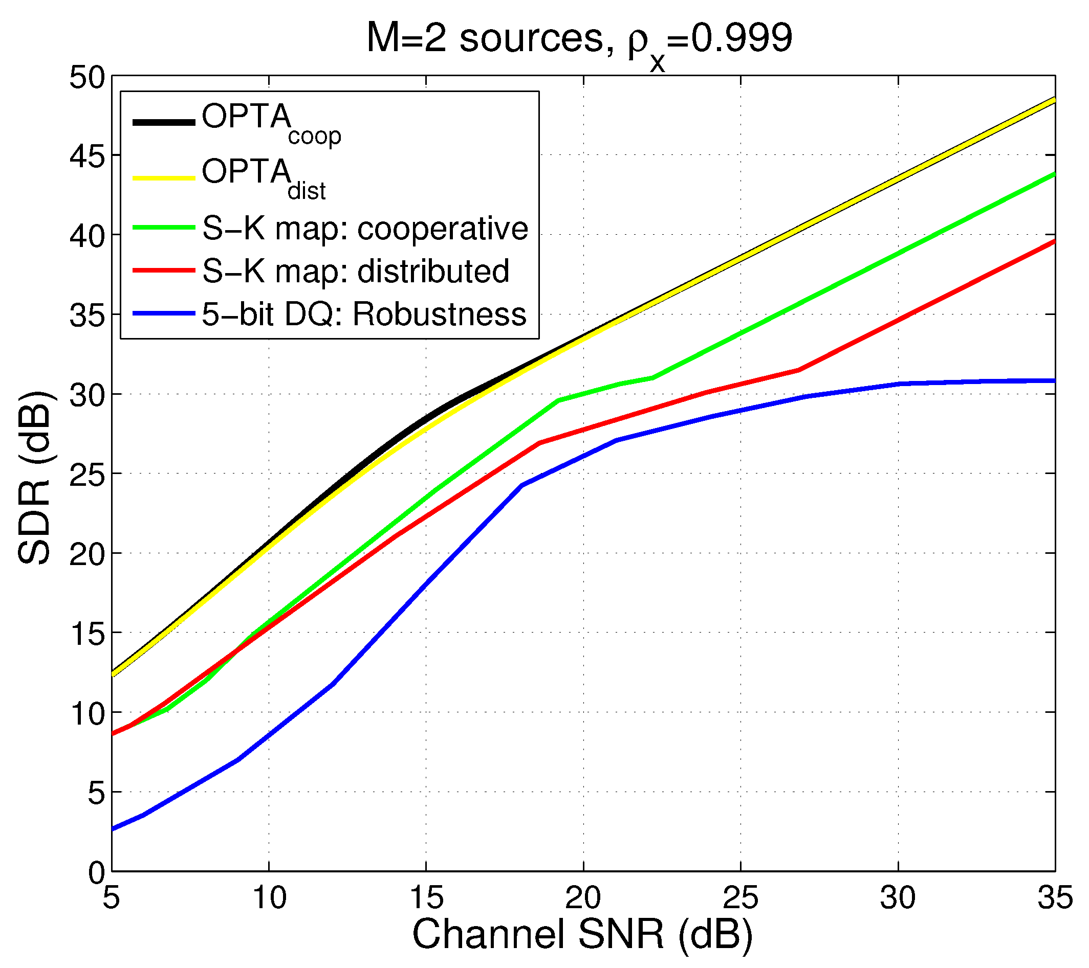
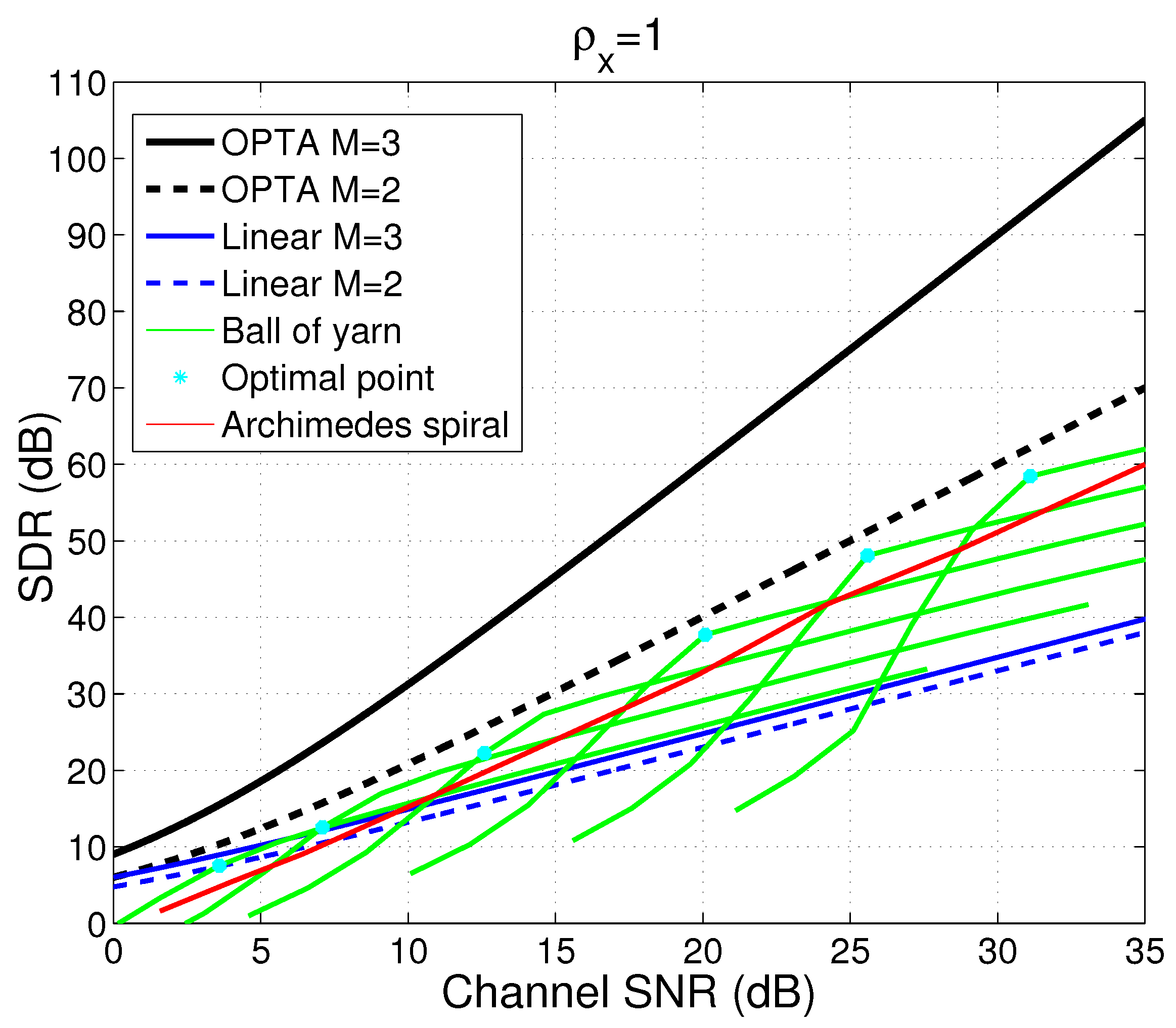
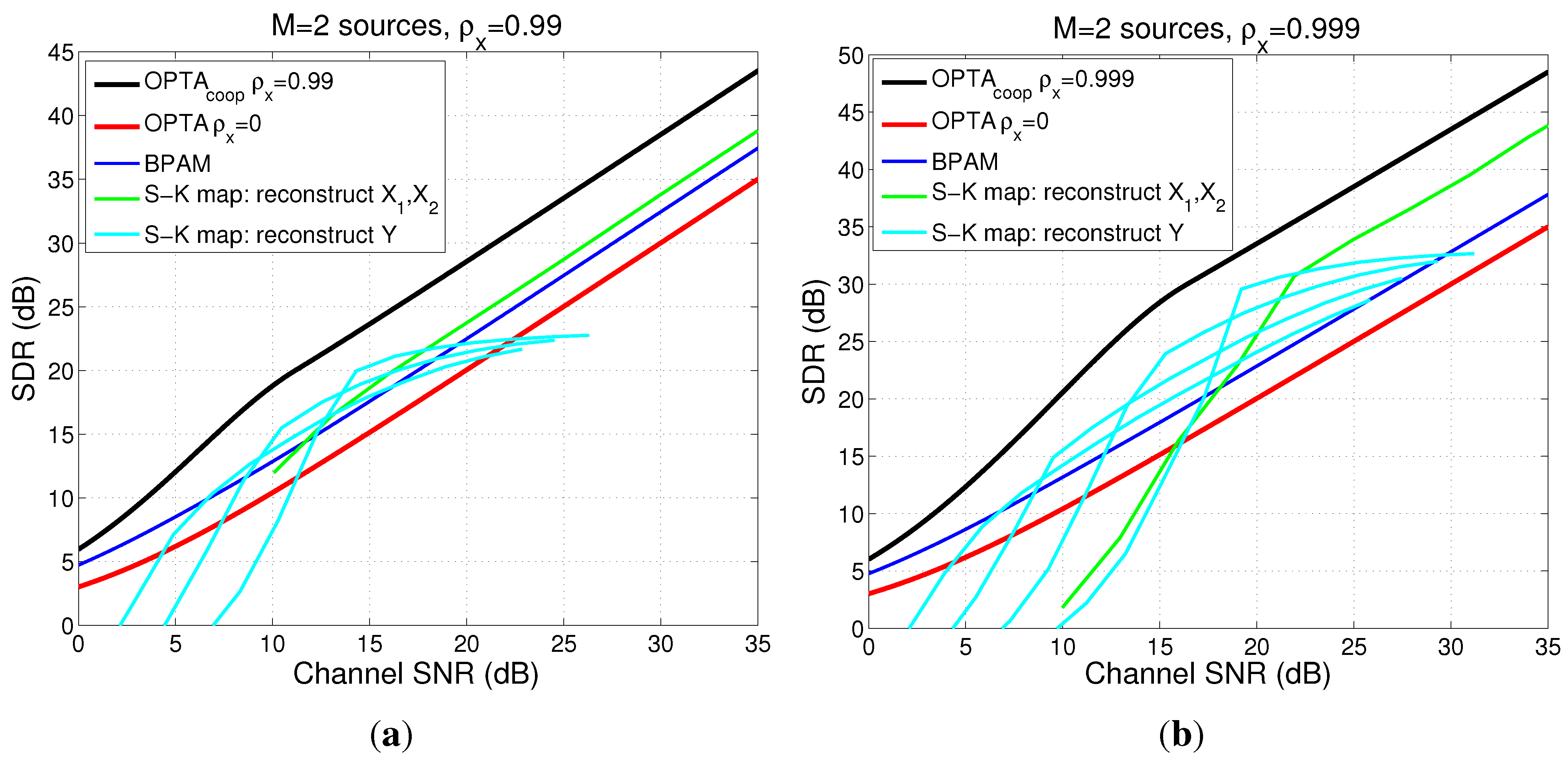
4.5.3. Comparison Between Collaborative Case, Distributed Case and DQ

Figure 12 shows a comparison between the optimal performance of all the suggested cooperative and distributed S-K mappings and 5-bit DQ from [9] optimized at 18 dB SNR.
Figure 12. Comparison of cooperative S-K mappings, distributed S-K mappings and 5-bit DQ for M = 2 when ρ x = 0 . 999 . DQ is optimized for 18 dB SNR.
Entropy 15 02129 g012
There is a clear gain from collaboration for SNR above 8 dB. The reason why collaboration helps when only common information is decoded is that z 1 and z 2 can be removed prior to transmission, and thereby reduce the probability for anomalous errors. The fact that z 1 and z 2 cannot be removed with distributed encoders may be one possible explanation why the OPTA bounds for the distributed and cooperative case differ. For higher SNR, when both common information, as well as individual observations are decoded, there is still a clear gain from collaborative encoders. A probable reason is that the generalized spiral utilizes the available space better than the sawtooth mapping as ρ x approaches one (at least with Gaussian statistics). The question is if there exists better zero delay distributed mappings that can close the gap to the cooperative case at high SNR (the OPTA bounds are at least the same at a high SNR). DQ is around 2 dB inferior to the distributed S-K mappings at its optimal point (17 dB). With a higher number of bits in the DQ encoders, one would expect the DQ to become at least as good as the distributed S-K mapping. Note that the difference between these three cases is smaller when ρ x = 0 . 99 .
Note that when ρ x gets smaller than about = 0 . 95 , the DQ optimization algorithm in [9] only generates quantized linear mappings. This corresponds to what happens with S-K mappings: When ρ x drops below a certain value, the source space will be too “wide” to be twisted into the channel space by a nonlinear S-K mapping. Either the channel power constraint will be violated or a myriad of anomalous errors would be introduced.

4.6. Extensions

A particular case that needs further investigation is the distributed case when correlation is around 0 < ρ x < 0 . 95 . The only known zero delay JSCC applicable (to our knowledge) for this case is distributed linear schemes, which provide no gain compared to the non-correlated case when SNR is large (see Figure 2). To avoid this problem, one can look for nonlinear alternatives that may provide better performance than linear mappings at zero delay. Whether such alternatives can be found or not must be determined through further research. Alternatively, one will have to increase the code length beyond one.
The DQ algorithm discussed in Section 4.5.3. is built on uniform quantization, and it is likely that additional gains can be achieved when 0 < ρ x < 0 . 95 by applying nonuniform quantization. The continuous analogy of this would be an exchange of the linear encoder in Equation (9), with a nonlinear one-to-one “stretching” function, φ ( x m ) , that changes the coordinate grids along each dimension in a nonlinear way. This would result in g i i ’s better tailored to a Gaussian distribution. Then, weak noise distortion could be made somewhat smaller without bending or twisting the source space (unlike the nonlinear mappings suggested in this paper). Anomalous errors are then avoided, and the power constraint is satisfied. The optimal g 11 was determined for a 1:N mapping in [48] (pp. 294–297) using variational calculus. An extension of this result to include several g i i could be applied for our purpose. Instead of letting all encoders be nonlinear, one may possibly achieve a gain by letting φ ( x m ) be linear for some of the encoders and nonlinear for the others, then apply optimal power allocation among all the encoders. Further research is needed to come to a conclusion, however.
How could one go about extending the nonlinear schemes in this paper beyond zero delay? Piecewise continuous mappings, like the Sawtooth mapping, have already been extended [10] using known lattice structures. At the time of writing, we know of no such tools for fully continuous mappings. Fully continuous mappings can be extended conceptually, however, as we illustrated for i.i.d. sources in [38]. Take the generalized spiral in Equation (25) as an example. The spiral, h , could be generalized to a two-dimensional “spiral like” surface that map two and two samples of y a at each time instant. One could further map two and two samples of z a along the two normal vectors of h . The difficult part is to determine the equation for the surface h , since when h is found, its normal vectors are determined by Equation (63). It might be possible to find such extensions of h when the codelength is small, but this will be notoriously difficult when the codelength is large. For practical reasons, it is therefore likely that fully continuous nonlinear mappings are applicable at low delay only.

5. Summary, Conclusions and Future Work

In this paper, delay-free joint source channel coding (JSCC) for communication of multiple inter-correlated memoryless Gaussian sources over orthogonal additive white Gaussian noise channels was investigated. Both ideally collaborating and distributed encoders were studied for the case where all sources should be reconstructed at the decoder.
First, optimal linear JSCC were investigated. With collaborative encoders, one may decorrelate the sources then allocate power optimally among the encoders. This provides an increase in received fidelity with increasing correlation. For the distributed case, however, it is impossible to decorrelate the sources, implying that no gain in fidelity can be achieved with distributed linear schemes when correlation increases if the channel SNR is high. Nonlinear JSCC, on the other hand, can provide significant gains in fidelity over all linear schemes when correlation is close to one for most SNR. Contrary to linear distributed schemes, carefully chosen nonlinear distributed schemes can provide an increasing gain in fidelity from increasing correlation also at high SNR. Since collaborative encoders offer more degrees of freedom in the choice of encoders, they can provide benefits over distributed encoders, except in the cases when correlation is zero. The zero correlation case is trivial and achieves the performance upper bounds (OPTA) with linear schemes. When the correlation is nonzero, all suggested schemes leave a gap to the performance upper bound, however. All schemes studied are robust towards changes in channel SNR.
Possible extensions of the work in this paper include increasing code length, unequal correlations between each encoder and unequal attenuation on each sub-channel. Nonlinear mapping that may provide better performance at intermediate correlation should also be investigated, and the gap to the performance upper bound should be quantified. Practical issues, like imperfect synchronization and timing, could also be investigated.

Acknowledgments

This work was supported by the Research Council of Norway (NFR), under the projects MELODY II nr. 225885/O70, ASSET nr. 213131 and CROPS nr. 181530/S10.

Appendix

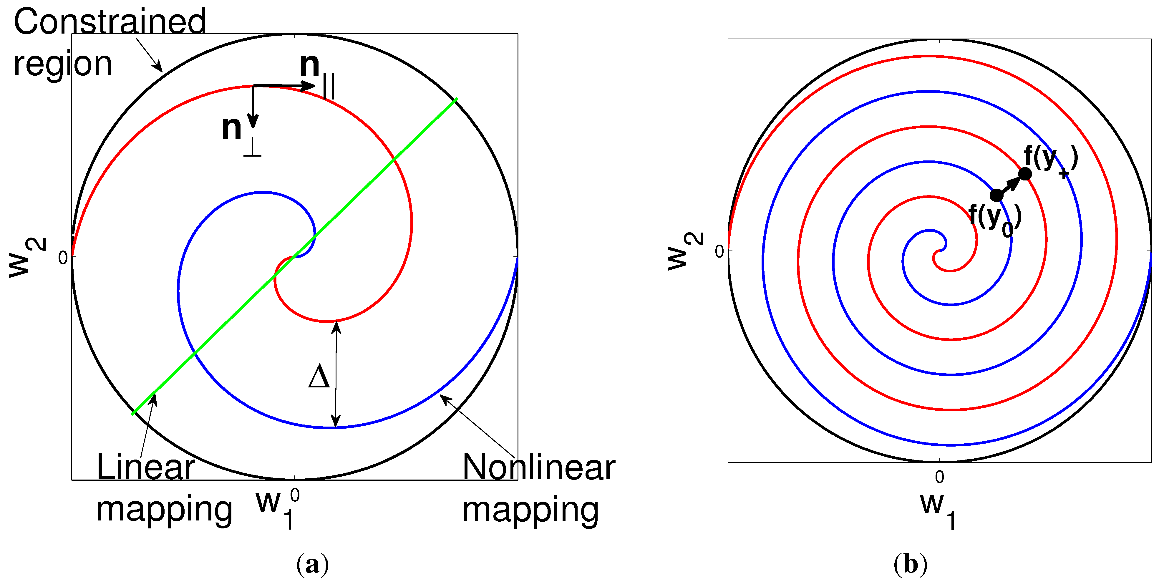
A. Normal Vector for Archimedes Spiral

The unit normal vector for a curve, f ( y ) , can be determined from the tangent vector, v ( y ) = f ( y ) . Let T = v ( y ) / v ( y ) and:
s = a b f 1 ( y ) 2 + f 2 ( y ) 2 d y
be the curve length of f . The unit normal vector is then given by [49] (chapter 12):
N = d T d s 1 K
where K = d T / d s is the curvature of f . By calculating Equation (63) for the functions in Equation (21) with a = 1 , then Equation (26) results.

B. Metric Tensor

Consider an M-dimensional parametric hyper-surface, f ( x ) . The metric tensor (also called a Riemannian Metric) for a smooth embedding of f in R N ( M N ) can be described by the symmetric and positive definite matrix [50] (chapter 9):
G = J T J = g 11 g 12 g 1 M g 21 g 22 g 2 M g M 1 g M 2 g M M
where J is the Jacobian of f , given by:
J = f 1 x 1 f 2 x 1 f N x 1 f 1 x 2 f 2 x 2 f N x 2 f 1 x M f 2 x M f N x M T
g i i can be interpreted as the squared norm of the tangent vector along f ( x i ) , where x i can be seen as the i’th parameter in the parametrization, f . All cross terms, g i j , are the inner product of tangent vectors along f ( x i ) and f ( x j ) . See, e.g., [50] (chapter 9) for further details.
Note that the metric tensor is an intrinsic feature of a manifold/hypersurface. That is, it describes local properties of a manifold/hypersurface without any dependence on an external coordinate system.

References

  1. Slepian, D.; Wolf, J.K. Noiseless coding of correlated information sources. IEEE Trans. Inf. Theory 1973, 19, 471–480. [Google Scholar] [CrossRef]
  2. Berger, T. Rate Distortion Theory: A Mathematical Basis for Data Compression; Prentice-Hall: Englewood Cliffs, NJ, USA, 1971. [Google Scholar]
  3. Oohama, Y. The rate-distortion function for the quadratic Gaussian CEO problem. IEEE Trans. Inf. Theory 1998, 44, 1057–1070. [Google Scholar] [CrossRef]
  4. Oohama, Y. Gaussian multiterminal source coding. IEEE Trans. Inf. Theory 1997, 43, 1912–1923. [Google Scholar] [CrossRef]
  5. Wagner, A.B.; Tavildar, S.; Viswanath, P. Rate region of the quadratic Gaussian two-encoder source-coding problem. IEEE Trans. Inf. Theory 2008, 54, 1938–1961. [Google Scholar] [CrossRef]
  6. Oohama, Y. Distributed source coding for correlated memoryless Gaussian sources. 2010; arXiv:0908.3982v4 [cs.IT]. [Google Scholar]
  7. Ray, S.; Medard, M.; Effros, M.; Kotter, R. On separation for multiple access channel. In Proceedings of IEEE Information Theory Workshop, Chengdu, China, 22–26 October 2006; pp. 399–403.
  8. Wernersson, N.; Skoglund, M. Nonlinear coding and estimation for correlated data in wireless sensor networks. IEEE Trans. Commun. 2009, 57, 2932–2939. [Google Scholar] [CrossRef]
  9. Wernersson, N.; Karlsson, J.; Skoglund, M. Distributed quantization over noisy channels. IEEE Trans. Commun. 2009, 57, 1693–1700. [Google Scholar] [CrossRef]
  10. Karlsson, J.; Skoglund, M. Lattice-based source-channel coding in wireless sensor networks. In Proceedings of IEEE International Conferece on Communications, Kyoto, Japan, 5–9 June 2011; pp. 1–5.
  11. Akyol, E.; Rose, K.; Ramstad, T.A. Optimized analog mappings for distributed source-channel coding. In Proceedings of IEEE Data Compression Conference, Snowbird, Utah, USA, 24–26 March 2010; pp. 159–168.
  12. Gastpar, M.; Dragotti, P.L.; Vetterli, M. The distributed Karhunen-Loeve transform. IEEE Trans. Inf. Theory 2006, 52, 5177–5196. [Google Scholar] [CrossRef]
  13. Rajesh, R.; Sharma, N. Correlated Gaussian sources over orthogonal Gaussian channels. In Proceedings of International Symposium on Information Theory and its Applications, Auckland, New Zealand, 7–10 December 2008; pp. 1–6.
  14. Lapidoth, A.; Tinguely, S. Sending a bi-variate Gaussian over a Gaussian MAC. IEEE Trans. Inf. Theory 2010, 60, 2714–2752. [Google Scholar] [CrossRef]
  15. Floor, P.A.; Kim, A.; Wernersson, N.; Ramstad, T.; Skoglund, M.; Balasingham, I. Zero-delay joint source-channel coding for a bi-variate Gaussian on a Gaussian MAC. IEEE Trans. Commun. 2012, 60, 3091–3102. [Google Scholar] [CrossRef]
  16. Vaishampayan, V.A. Combined source-channel coding for bandlimited waveform channels. Ph.D. dissertation, University of Maryland, MD, USA, 1989. [Google Scholar]
  17. Shannon, C.E. Communication in the presence of noise. Proc. IRE 1949, 37, 10–21. [Google Scholar] [CrossRef]
  18. Kotel’nikov, V.A. The Theory of Optimum Noise Imunity; McGraw-Hill Book Company: New York, NY, USA, 1959. [Google Scholar]
  19. Goblick, T.J. Theoretical limitations on the transmission from analog sources. IEEE Trans. Inf. Theory 1965, 11, 558–567. [Google Scholar] [CrossRef]
  20. McRae, D. Performance evaluation of a new modulation technique. IEEE Trans. Inf. Theory 1970, 16, 431–445. [Google Scholar] [CrossRef]
  21. Timor, U. Design of signals for analog communication. IEEE Trans. Inf. Theory 1970, 16, 581–587. [Google Scholar] [CrossRef]
  22. Thomas, C.; May, C.; Welti, G. Hybrid amplitude-and-phase modulation for analog data transmission. IEEE Trans. Commun. 1976, 23, 634–645. [Google Scholar] [CrossRef]
  23. Lee, K.H.; Petersen, D.P. Optimal linear coding for vector channels. IEEE Trans. Commun. 1976, 24, 1283–1290. [Google Scholar]
  24. Fuldseth, A.; Ramstad, T.A. Bandwidth compression for continuous amplitude channels based on vector approximation to a continuous subset of the signal space. In Proceedings of IEEE International Conference on Acoustics, Speech, and Signal Processing, Atlanta, GA, USA, 21–24 April 1997; pp. 3093–3096.
  25. Coward, H.; Ramstad, T.A. Quantizer optimization in hybrid digital-analog transmission of analog source signals. In Proceedings of IEEE International Conference on Acoustics, Speech, and Signal Processing, Istanbul, Turkey, 5–9 June 2000; pp. 2637–2640.
  26. Chung, S.Y. On the construction of some capacity-approaching coding schemes. Ph.D. dissertation, Massachusetts Institute of Technology, MA, USA, 2000. [Google Scholar]
  27. Ramstad, T.A. Shannon mappings for robust comunication. Telektronikk 2002, 98, 114–128. [Google Scholar]
  28. Mittal, U.; Phamdo, N. Hybrid digital-analog (HDA) joint source-chanel codes for broadcasting and robust communications. IEEE Trans. Inf. Theory 2002, 48, 1082–1102. [Google Scholar] [CrossRef]
  29. Gastpar, M.; Rimoldi, B.; Vetterli, M. To code, or not to code: Lossy source-channel communication revisited. IEEE Trans. Inf. Theory 2003, 49, 1147–1158. [Google Scholar] [CrossRef]
  30. Skoglund, M.; Phamdo, N.; Alajaji, F. Hybrid digital-analog source-chanel coding for bandwidth compression/expansion. IEEE Trans. Inf. Theory 2006, 52, 3757–3763. [Google Scholar] [CrossRef]
  31. Hekland, F.; Floor, P.A.; Ramstad, T.A. Shannon-Kotel’nikov mappings in joint source-channel coding. IEEE Trans. Commun. 2009, 57, 94–105. [Google Scholar] [CrossRef]
  32. Floor, P.A.; Ramstad, T.A. Optimality of dimension expanding Shannon-Kotel’nikov mappings. In Proceedings of IEEE Information Theory Workshop, Tahoe City, CA, USA, 2–6 September 2007; pp. 289–294.
  33. Cai, X.; Modestino, J.W. Bandwidth expansion Shannon mapping for analog error-control coding. In Proceedings of IEEE Conference on Information Sciences and Systems, Princeton University, Princeton, NJ, USA, 22–24 March 2006; pp. 1709–1712.
  34. Akyol, E.; Rose, K.; Ramstad, T.A. Optimal mappings for joint source channel coding. In Proceedings of IEEE Information Theory Workshop, Dublin, Ireland, 30 August–3 September 2010; pp. 1–5.
  35. Hu, Y.; Garcia-Frias, J.; Lamarca, M. Analog joint source-channel coding using non-linear curves and MMSE decoding. IEEE Trans. Commun. 2011, 59, 3016–3026. [Google Scholar] [CrossRef]
  36. Erdozain, A.; Crespo, P.M.; Beferull-Lozano, B. Multiple description analog joint source-chanel coding to exploit the diversity in parallel channels. IEEE Trans. Signal Proc. 2012, 60, 5880–5892. [Google Scholar] [CrossRef]
  37. Kochman, Y.; Zamir, R. Analog matching of colored sources to colored channels. IEEE Trans. Inf. Theory 2011, 57, 3180–3195. [Google Scholar] [CrossRef]
  38. Floor, P.A.; Ramstad, T.A. Shannon-Kotel’nikov mappings for analog point-to-point communications. 2012; arXiv:1101.5716v2 [cs.IT]. [Google Scholar]
  39. Kim, A.; Floor, P.A.; Ramstad, T.A.; Balasingham, I. Delay-free joint source-channel coding for Gaussian network of multiple sensors. In Proceedings of IEEE International Conferece on Communications, Kyoto, Japan, 5–9 June 2011; pp. 1–6.
  40. Wozencraft, J.M.; Jacobs, I.M. Principles of Communication Engineering; John Wiley & Sons: New York, NY, USA, 1965. [Google Scholar]
  41. Floor, P.A.; Ramstad, T.A. Dimension reducing mappings in joint source-channel coding. In Proceedings of IEEE Nordic Signal Processing Symposium, Reykjavik, Iceland, 7–9 June 2006; pp. 282–285.
  42. Saleh, A.A.; Alajaji, F.; Chan, W.Y. Hybrid digital-analog source-channel coding with one-to-three bandwidth expansion. In Proceedings of IEEE Canadian Workshop in Information Theory, Kelowna, Canada, 17–20 May 2011; pp. 70–73.
  43. Merhav, N. Threshold effects in parameter estimation as phase transitions in statistical mechanics. IEEE Trans. Inf. Theory 2011, 57, 7000–7010. [Google Scholar] [CrossRef]
  44. Cramér, H. Mathematical Methods of Statistics; Princeton University Press: Princeton, NJ, USA, 1951. [Google Scholar]
  45. Cover, T.A.; Thomas, J.A. Elements of Information Theory; John Wiely & Sons: New York, NY, USA, 1991. [Google Scholar]
  46. Papoulis, A.; Pillai, S.U. Probability, Random Variables and Stochastic Processes; McGraw-Hill: New York, NY, USA, 2002. [Google Scholar]
  47. Gasquet, C.; Witomski, P. Fourier Analysis and Applications; Springer-Verlag: New York, NY, USA, 1999. [Google Scholar]
  48. Sakrison, D.J. Communication Theory: Transmission of Waveforms and Digital Infromation; John Wiley & Sons: New York, NY, USA, 1968. [Google Scholar]
  49. Edwards, C.H.; Penney, D.E. Calculus with Analytic Geometry; Prentice Hall International Inc.: Upper Saddle River, NJ, USA, 1998. [Google Scholar]
  50. Spivak, M. A Comprehensive Introduction to Differential Geometry; Publish or Perish: Huston, TX, USA, 1999. [Google Scholar]

