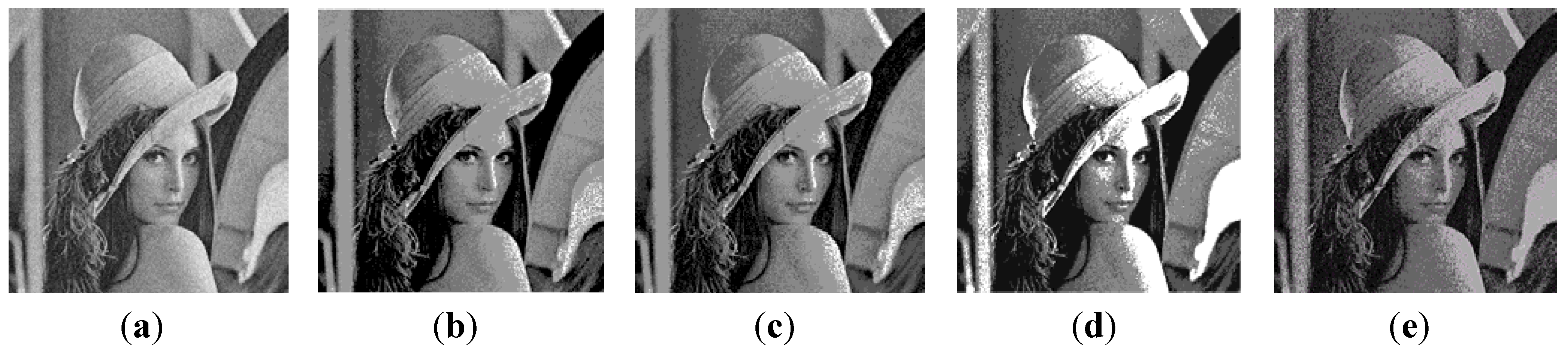
Article

An Automatic Multilevel Image Thresholding Using Relative Entropy and Meta-Heuristic Algorithms

Department of Industrial Engineering and Management, Yuan Ze University, 320, Taiwan
*
Author to whom correspondence should be addressed.
Entropy 2013, 15(6), 2181-2209; https://doi.org/10.3390/e15062181
Submission received: 1 March 2013 / Revised: 3 May 2013 / Accepted: 23 May 2013 / Published: 3 June 2013

Abstract

:
Multilevel thresholding has been long considered as one of the most popular techniques for image segmentation. Multilevel thresholding outputs a gray scale image in which more details from the original picture can be kept, while binary thresholding can only analyze the image in two colors, usually black and white. However, two major existing problems with the multilevel thresholding technique are: it is a time consuming approach, i.e., finding appropriate threshold values could take an exceptionally long computation time; and defining a proper number of thresholds or levels that will keep most of the relevant details from the original image is a difficult task. In this study a new evaluation function based on the Kullback-Leibler information distance, also known as relative entropy, is proposed. The property of this new function can help determine the number of thresholds automatically. To offset the expensive computational effort by traditional exhaustive search methods, this study establishes a procedure that combines the relative entropy and meta-heuristics. From the experiments performed in this study, the proposed procedure not only provides good segmentation results when compared with a well known technique such as Otsu’s method, but also constitutes a very efficient approach.

Graphical Abstract

1. Introduction

Segmenting an image into its constituents is a process known as thresholding [1,2]. Those constituents are usually divided into two classes: foreground (significant part of the image), and background (less significant part of the image). Several methods for thresholding an image have been developed over the last decades, some of them based on entropy, within and between group variance, difference between original and output images, clustering, etc. [3,4,5].
The process of thresholding is considered as the simplest image segmentation method, which is true when the objective is to convert a gray scale image into a binary (black and white) one (that is to say only one threshold is considered). However, in the process of segmentation, information from the original image will be lost if the threshold value is not adequate. This problem may even deteriorate as more than one threshold is considered (i.e., multilevel thresholding) since not only a proper number of thresholds is desirable, but also a fast estimation of their values is essential [1].
It has been proven over the years that as more thresholds are considered in a given image, the computational complexity of determining proper values for each threshold increases exponentially (when all possible combinations are considered). Consequently, this is a perfect scenario for implementing meta-heuristic tools [6] in order to speed up the computation and determine proper values for each threshold.
When dealing with multilevel thresholding, in addition to the fast estimation, defining an adequate number of levels (thresholds that will successfully segment the image into several regions of interest from the background), has been another problem without a satisfactory solution [7]. Therefore, the purpose and main contribution of this study is to further test the approach proposed in [8] which determines the number of thresholds necessary for segmenting a gray scaled image automatically. The aforementioned is achieved by optimizing a mathematical model based on the Relative Entropy Criterion (REC).
The major differences between this work and the one presented in [8], are that a more extensive and comprehensive testing of the proposed method was carried out. To verify the feasibility of the proposed model and reduce the computational burden, when carrying out the optimization process, this study implements three meta-heuristic tools and compares the output images with that delivered by a widely known segmentation technique named Otsu’s method. In addition to the aforementioned, further tests with images having low contrast and random noise are conducted; this intends to probe the robustness, effectiveness and efficiency of the proposed approach.
The following paper is organized as follows: Section 2 introduces the proposed procedure, which consists of the mathematical model based on the relative entropy and the meta-heuristics—virus optimization algorithm, genetic algorithm, and particle swarm optimization as the solution searching techniques. Section 3 illustrates the performance of the proposed method when the optimization is carried out by three different algorithms VOA, GA and PSO, where six different types of images were tested. Lastly, some concluding remarks and future directions for research are provided in Section 4.

2. The Proposed Multilevel Thresholding Method

A detailed explanation of the proposed method is given in this section, where the mathematical formulation of the model is presented and the optimization techniques are introduced.

2.1. Kullback-Leibler Information Distance (Relative Entropy)

The Kullback-Leibler information distance (known as Relative Entropy Criterion) [9] between the true and the fitted probabilities is implemented in [8] for estimating an appropriate model that will best represent the histogram coming from the gray level intensity of an image. According to McLachlan and Peel [10] this information distance is defined as in Equation (1). However, the gray levels (intensity) are discrete values between [0, 255]; therefore, Equation (1) can be rewritten as in Equation (2):
J ( d ) = I { p ( i ) ; p ( i ; θ d ) } = ( p ( i ) log e [ p ( i ) p ( i ; θ d ) ] ) d i
J ( d ) = I { p ( i ) ; p ( i ; θ d ) } = i = 0 255 ( p ( i ) log e [ p ( i ) p ( i ; θ d ) ] )
where p(i) and p(i;θd) are the probabilities values from the image histogram and fitted model respectively. These probabilities are estimated using Equations (3) and (4), where the value of i [ 0 ,     255 ] and represents the gray intensity of a pixel at location (x, y) on the image of size M × N pixels; while j = 1 d g ( i , θ j ) in Equation (4) is a mixture of “d” distributions which are used to estimate the value of p(i;θd). Lastly, θj is a vector containing the parameters of each distribution in the mixture:
p ( i ) = T o t a l   n u m b e r   o f   p i x e l s   w i t h   g r a y   i n t e s i t y   o f   i S i z e   o f   t h e   i m a g e
p ( i ; θ d ) = g ( i , θ 1 ) + + g ( i , θ d ) = j = 1 d g ( i , θ j )
In this study Gaussian distributions are used to estimate Equation (4), where the central limit theorem (C.L.T.) is the motivation of using this type of distributions [11]. Therefore, Equation (4) can be expressed as in Equation (5):
p ( i ; θ d ) = j = 1 d ( w j 2 π σ j e   1 2 [ ( i μ j σ j ) 2 ] )
where θj contains the prior probability (or weight) wj, mean μj, and variance σ2j, of the jth Gaussian distribution. The minimization of the Relative Entropy Criterion function can be interpreted as the distance reduction between the observed and estimated probabilities. This should provide a good description of the observed probabilities p(i) given by the gray level histogram of the image under study. However, finding an appropriate number of distributions, i.e., “d”, is a very difficult task [12,13,14,15]. Consequently, the addition of a new term in Equation (2), which is detailed in the following subsection helps to automatically determine a suitable amount of distributions.

2.2. Assessing the Number of Distributions in a Mixture Model

The purpose of assuming a mixture of “d” distributions in order to estimate p(i;θd) in the REC function, is that the number of thresholds for segmenting a given image, can be easily estimated using Equation (6). The value of each threshold is the gray level intensity “i” that minimizes Equation (7), where “i” is a discrete unit (i.e., an integer [0, 255]):
n u m b e r   o f   t h r e s h o l d s = d 1
T h r e s h o l d k = arg min i { | p ( i ; θ k ) p ( i ; θ k + 1 ) | }      k = 1 , 2 , ... , d 1
Given that estimating a suitable number of distributions “d” is a very difficult task, the method proposed in [8] attempts to automatically assess an appropriate value for “d” combining Equations (2) and (8) as a single objective function. The vector w contains all the prior probabilities (weights) of the mixture model. The values max(w) and min(w) are the maximum and minimum weights in w respectively:
P ( d ) = 1 d 1 j = 1 d ( max ( w ) w j max ( w ) min ( w ) )
Equation (8) compares each prior probability wj with respect to the largest one in the vector w. The result is normalized using the range given by [max(w)–min(w)] in order to determine how significant wj is with respect to the probability that contributes the most in the model, i.e., max(w). Therefore, Equation (8) will determine if the addition of more Gaussian distributions is required for a better estimation of p(i;θd). The term 1 d 1 will avoid Equation (8) overpowering Equation (2) when the mathematical model of Equation (9) is minimized:
Θ ( d ) = i = 0 255 ( p ( i ) log e [ p ( i ) p ( i ; θ d ) ] ) + 1 d 1 j = 1 d ( max ( w ) w j max ( w ) min ( w ) )
Therefore, by minimizing Equation (9), the introduced approach will not only determine an appropriate number of distributions in the mixture model, but will also find a good estimation (fitting) of the probabilities p(i) given by the image histogram. An appropriate value for “d” is determined by increasing its value by one, i.e., dl = dl−1 + 1 where “l” is the iteration number, and minimizing Equation (9) until a stopping criterion is met and the addition of more distributions to the mixture model is not necessary. Therefore, not all the possible values for “d” are used.

2.3. Mathematical Model Proposed for Segmenting (Thresholding) a Gray Level Image

The mathematical model which is used for segmenting a gray level image is presented as in Equation (10). By minimizing Equation (10) with “d” Gaussian distributions, J(d) is in charge of finding a good estimation (fitting) of the image histogram, while P(d) determines whenever the addition of more distributions to the model is necessary:
M i n   Θ ( d ) = M i n [ J ( d ) + P ( d ) ] = M i n θ d , d [ i = 0 255 ( p ( i ) log e [ p ( i ) p ( i ; θ d ) ] ) + 1 d 1 j = 1 d ( max ( w ) w j max ( w ) min ( w ) ) ]
subject to:
j = 1 d w j = 1
w j > 0    j [ 1 , d ]
σ j 2 > 0    j [ 1 , d ]
Equation (11) guarantees a summation of the prior probabilities equal to 1, while Equations (12) and (13) ensure positive values to all prior probabilities and variances in the mixture model, respectively. To minimize Equation (10), a newly developed meta-heuristic named Virus Optimization Algorithm [16], the widely known Genetic Algorithm [17] and Particle Swarm Optimization algorithm [18] are implemented in this study.
The flowchart at Figure 1 details the procedure of the proposed method using VOA (the similar idea is also applied to GA and PSO). As can be observed, the optimization tool (VOA, GA, or PSO) will optimize Equation (10) with dl Gaussian distributions until the stopping criterion of the meta-heuristic is reached. Once the algorithm finishes optimizing Equation (10) with dl distributions, the proposed method decides if the addition of more components is necessary if and only if Θ(dl) Θ(dl−1) is true; otherwise a suitable number of distributions (thresholds) just been found and the results coming from Θ(dl−1) are output.
The purpose of using three algorithmic tools, is not only to reduce the computation time when implementing the proposed approach, but also, to verify if the adequate number of thresholds suggested by optimizing Equation (10) with different optimization algorithm remains the same. The reason of the aforementioned is because different algorithms may reach different objective function values. However, if the proposed method (Figure 1) is robust enough, all algorithms are expected to stop iterating when reaching a suitable number of thresholds, and this number has to be the same for all the optimization algorithms.

2.4. Algorithmic Optimization Tools

2.4.1. Virus Optimization Algorithm (VOA)

Inspired from the behavior of a virus attacking a host cell, VOA [8,16] is a population-based method that begins the search with a small number of viruses (solutions). For continuous optimization problems, a host cell represents the entire multidimensional solution space, where the cell’s nucleolus denotes the global optimum. Virus replication indicates the generation of new solutions while new viruses represent those created from the strong and common viruses.
The strong and common viruses are determined by the objective function value of each member in the population of viruses, i.e., the better the objective function value of a member the higher the chance to be considered as strong virus. The number of strong viruses is determined by the user of the algorithm, which we recommend to be a small portion of the whole population (strong and common).
Figure 1. Flowchart of the proposed optimization procedure.
Entropy 15 02181 g001
To simulate the replication process when new viruses are created, the population size will grow after one complete iteration. This phenomenon is controlled by the antivirus mechanism that is responsible for protecting the host cell against the virus attack. The whole process will be terminated based on the stopping criterion: the maximum number of iterations (i.e., virus replication), or the discovery of the global optimum (i.e., cell death is achieved).
The VOA consists of three main processes: Initialization, Replication, and Updating/Maintenance. The Initialization process uses the values of each parameter (defined by the user) to create the first population of viruses. These viruses are ranked (sorted) based on the objective function evaluation Θ(d) to select strong and common members. Here the number of strong members in the population of viruses is a parameter to be defined by the user, without considering the strong members; the population of viruses is the number of common viruses.
The replication process is performed using the parameters defined by the user in the Initialization stage described above, where a temporary matrix (larger than the matrix containing the original viruses) will hold the newly-generated members. Here, Equations (14) and (15) are used to generate new members, where “vn” stands for the value of the variable in the nth dimensional space, for viruses in the previous replication. “svn” stands for the value of the variable in the nth dimensional space generated from the strong viruses in the current replication, and “cvn” is the value of the variable in the nth dimensional space generated from the common viruses in the current replication:
s v n = v n ± ( r a n d ( ) intensity ) × v n
c v n = v n ± r a n d ( ) × v n
The intensity in Equation (14) above reduces the random perturbation that creates new viruses from the strong members. This will allow VOA to intensify exploitation in regions more likely to have a global optimum (i.e., areas where the strong viruses are located). The initial value for the intensity is set as one, which means that the random perturbation for strong and common viruses is the same in the early stages. Therefore, the exploration power of VOA is expected to be enhanced during the program’s early stages. The intensity value increases by one when the average performance of the population of viruses in VOA; that is to say, the average objective function value of the whole population of viruses, did not improve after a replication. The flowchart of the proposed procedure is illustrated in Figure 1. Note that the VOA part can be easily switched to other optimization algorithms such as GA and PSO.

2.4.2. Genetic Algorithm (GA)

The basic concept of Genetic Algorithms or GAs [17] is to simulate processes in natural systems, necessary for evolution, especially those that follows the principles first laid down by Charles Darwin of survival of the fittest. In GA a portion of existing population (solutions) is selected to breed a new population (new solutions), individuals are selected to reproduce (crossover) through a fitness-based process (objective function). Mutation takes place when new individuals are created after crossover to maintain a diverse population through generations. The standard GA is summarized in Figure 2, for the selection of the parents the roulette wheel is used in this study, as for the population maintenance mechanism the best members in the pooled population (parents and offspring) survive. The crossover operators implemented in this paper are the geometric and arithmetic means [Equations (16) and (17)] for the creation of the first and second child respectively. Note that only the integer part is taken by the program since the chromosome contains only integers. The mutation operator in GA uses Equation (18), which is the floor function of a random number generated between [Ti−1, Ti] where T0 = 0 and Td = 255:
T i c h i l d 1 = ( T i p a r e n t 1 + T i p a r e n t 2 ) 2 ,   i [ 1 , 2 , , d 1 ]
T i c h i l d 2 = ( T i p a r e n t 1 × T i p a r e n t 2 ) 1 2 ,   i [ 1 , 2 , , d 1 ]
T i = r a n d [ ( T i 1 + 1 ) , ( T i 1 ) ] ,   i [ 1 , 2 , , d ]
Figure 2. Genetic Algorithm (GA) overview.
Entropy 15 02181 g002

2.4.3. Particle Swarm Optimization (PSO)

Particle Swarm Optimization was inspired by social behavior of bird flocking or fish schooling [18]. Each candidate solution (known as particle) keeps track of its coordinates in the problem space which are associated with the best solution (fitness) it has achieved so far, also known as the particle’s best (pbest). The swarm on the other hand, also keeps track of the best value, obtained until now, by any particle in the neighbor of particles. This is known as the global best (gbest). The basic concept of PSO consists of changing the velocity of each particle towards the gbest and pbest location. This velocity is weighted by a random term, with separated random numbers being generated for acceleration toward the pbest and gbest locations. The standard PSO is summarized as in Figure 3. For this study, the velocity of the particle is bounded to a Vmax value which is only 2% of the gray intensity range; that is to say, Vi [−Vmax , Vmax] where Vmax = 0.02 × (255 − 0).
Figure 3. Overview of the Particle Swarm Optimization (PSO) algorithm.
Entropy 15 02181 g003
The stopping criterion for the VOA (GA or PSO) is when two consecutive replications (generations) did not improve the objective function value of the best virus (chromosome or particle). Once the VOA (GA or PSO) stops searching and the best value for the Θ(dl) is determined, the proposed method will decide if the addition of more distributions is necessary when the condition Θ(dl) < Θ(dl−1) is satisfied; otherwise the proposed method will automatically stop iterating. After the proposed method stops, the parameters contained inside the vector θdl-1 that represents the set of parameters of the best result in the previous iteration are output.
In order to avoid computational effort of calculating the threshold values that minimize Equation (7), the VOA (GA and PSO) will code each threshold value inside each solution, i.e., each virus (chromosome or particle) will have a dimensionality equal to the number of thresholds given by Equation (6). During the optimization, when the search of the best value for Θ(dl) is in process, each threshold will be treated as a real (not an integer) value, which can be considered as the coded solution of the VOA and PSO.
In the case of GA a chromosome containing integer values is used for encoding the solution. In order to evaluate the objective function of each virus or particle, the real values coded inside each member will be rounded to the nearest integer, whereas in GA this is not necessary since each chromosome is an array of integers. The parameters for each Gaussian distribution are computed as in Equations (19)–(21), which is considered as the decoding procedure of the three meta-heuristics implemented in this study:
w j = i = T j 1 T j p ( i ) ,      j [ 1 , d ]
μ j = i = T j 1 T j ( i × p ( i ) w j ) ,      j [ 1 , d ]
σ j 2 = i = T j 1 T j ( ( i μ j ) 2 × p ( i ) w j ) ,      j [ 1 , d ]
In Equations (19)–(21), Tj represents the jth threshold in the solution. The values for T0 = 0 and Td = 255, which are the lower and upper limits for thresholds values. During the optimization process, special care should be taken when generating new solutions (viruses, offspring, or particles). The details are as follows:
Condition 1: The threshold should be in increasing order when coded inside each solution, and two thresholds cannot have the same value, i.e., T0 < T1 < T2 <...< Td.
Condition 2: The thresholds are bounded by the maximum (Td = 255) and minimum (T0 = 0) intensity in a gray level image, i.e., 0 ≤ Tj ≤ 255, j [1, d−1].
Equation (22) is checked to ensure that the first condition is satisfied, where i, j [1, d−1] and i < j. If Equation (22) is not satisfied then the solution (virus, chromosome, or particle) is regenerated using Equation (23), where is the floor function. The second condition is also checked and whenever any threshold value is outside the boundaries, i.e., Tj 0 or Tj 255, the virus (chromosome or particle) is regenerated using Equation (23).
T i T j 0
V O A , P S O :   T i = ( r a n d ( ) × 255 d ) + ( ( i 1 ) × 255 d ) G A :   T i = ( r a n d ( ) × 255 d ) + ( ( i 1 ) × 255 d )

3. Experimental Results

In order to further test the method proposed in [8], five different types of images were tested. The first image, which has a known number of three thresholds as in this case is tested (Figure 4a); secondly, an image containing text on a wrinkled paper which will cause lighting variation is tested (Figure 5a). Thirdly, the Lena image (Figure 6a) [1,12,13,14,15] is tested, which is considered as a benchmark image when a new thresholding technique is proposed.
Figure 4. 
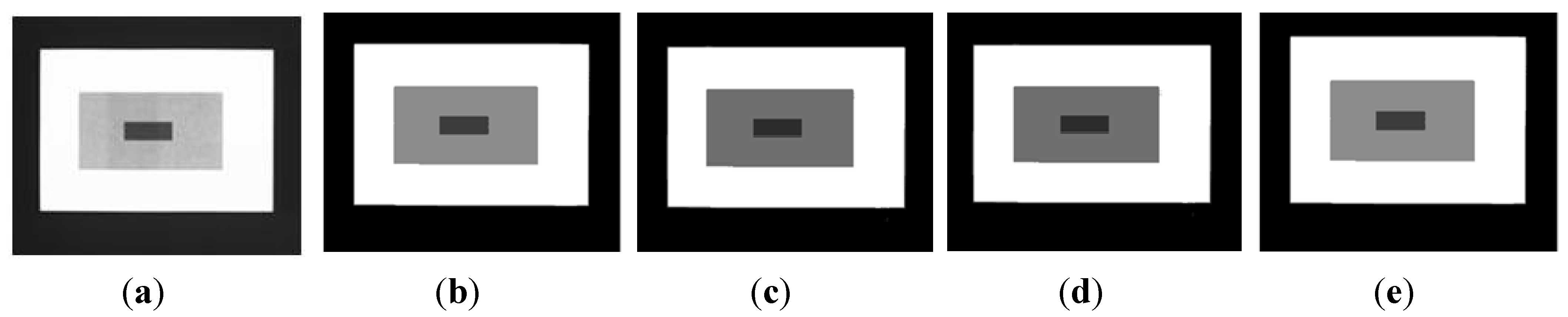
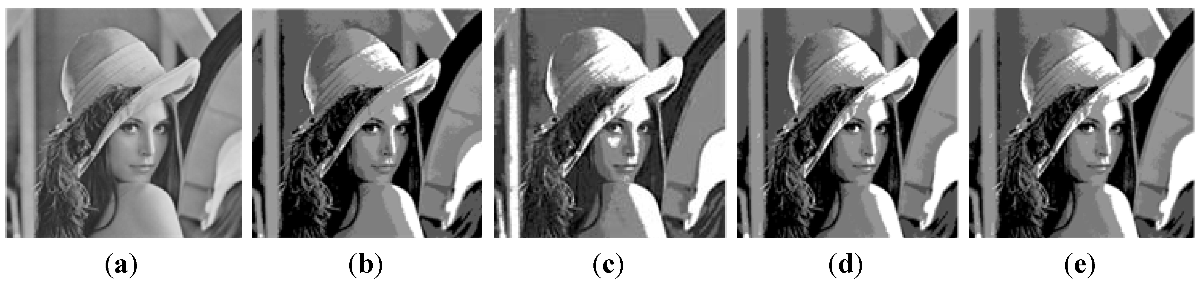
Test image 1: (a) Original image; Thresholded image implementing (b) VOA, (c) GA, (d) PSO, and (e) Otsu’s method using three thresholds.
Entropy 15 02181 g004
Figure 5. 
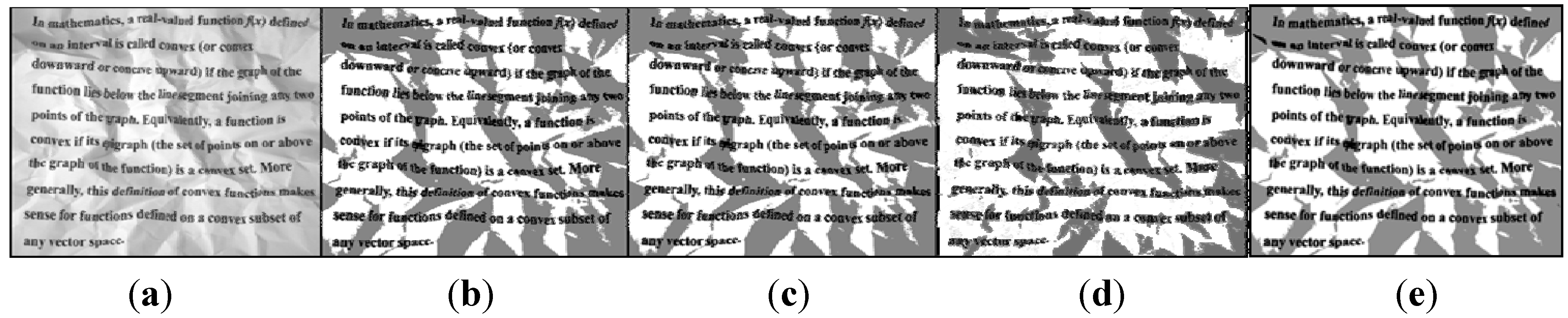
Test image 2: (a) Original image; Thresholded image implementing (b) VOA, (c) GA, (d) PSO, and (e) Otsu’s method with two thresholds.
Entropy 15 02181 g005
Figure 6. Test image 3: (a) Original image; Thresholded image implementing (b) VOA, (c) GA, (d) PSO, and (e) Otsu’s method with four thresholds. (taken from [1] )
Entropy 15 02181 g006

3.1. Algorithmic Setting (VOA, GA, and PSO)

The setting of VOA, GA, and PSO was determined by using Design of Experiments (DoE) [19,20] to know which values for the parameters are suitable when optimizing Equation (10). The full factorial design, i.e., 3-levels factorial design was performed for the four parameters of the VOA; in other words, 34 combinations of the four parameters were tested. Table 1 shows the results after performing DoE, where the final setting of the VOA is presented in bold.
Table 1. Parameter values (factor levels) used during the for the VOA.
ParameterLow Level Medium LevelHigh Level
Initial population of viruses51030
Viruses considered as strong1310
Growing rate of strong viruses2510
Growing rate of common viruses136
Similarly, a 33 full factorial design was implemented in order to set the population size (ps), crossover and mutation probabilities (pc and pm) respectively for GA. Table 2 summarizes the experimental settings and the final setting (in bold) of the GA. As for PSO a 34 full factorial design determined the values for the swarm size, inertia weight (w), cognitive and social parameters (c1 and c2) respectively. Table 3 summarizes the experimental settings of the PSO algorithm and the final setting is also highlighted in bold.
Table 2. Parameter values (factor levels) used during the DoE for the GA.
ParameterLow LevelMedium LevelHigh Level
Population size (ps)51030
Probability of crossover (pc)0.80.90.99
Probability of mutation (pm)0.050.10.15
Table 3. Parameter values (factor levels) used during the DoE for the PSO.
ParameterLow LevelMedium LevelHigh Level
Swarm size51030
Inertia weight (w)0.50.80.99
Cognitive parameter (c1)22.12.2
Social parameter (c2)22.12.2
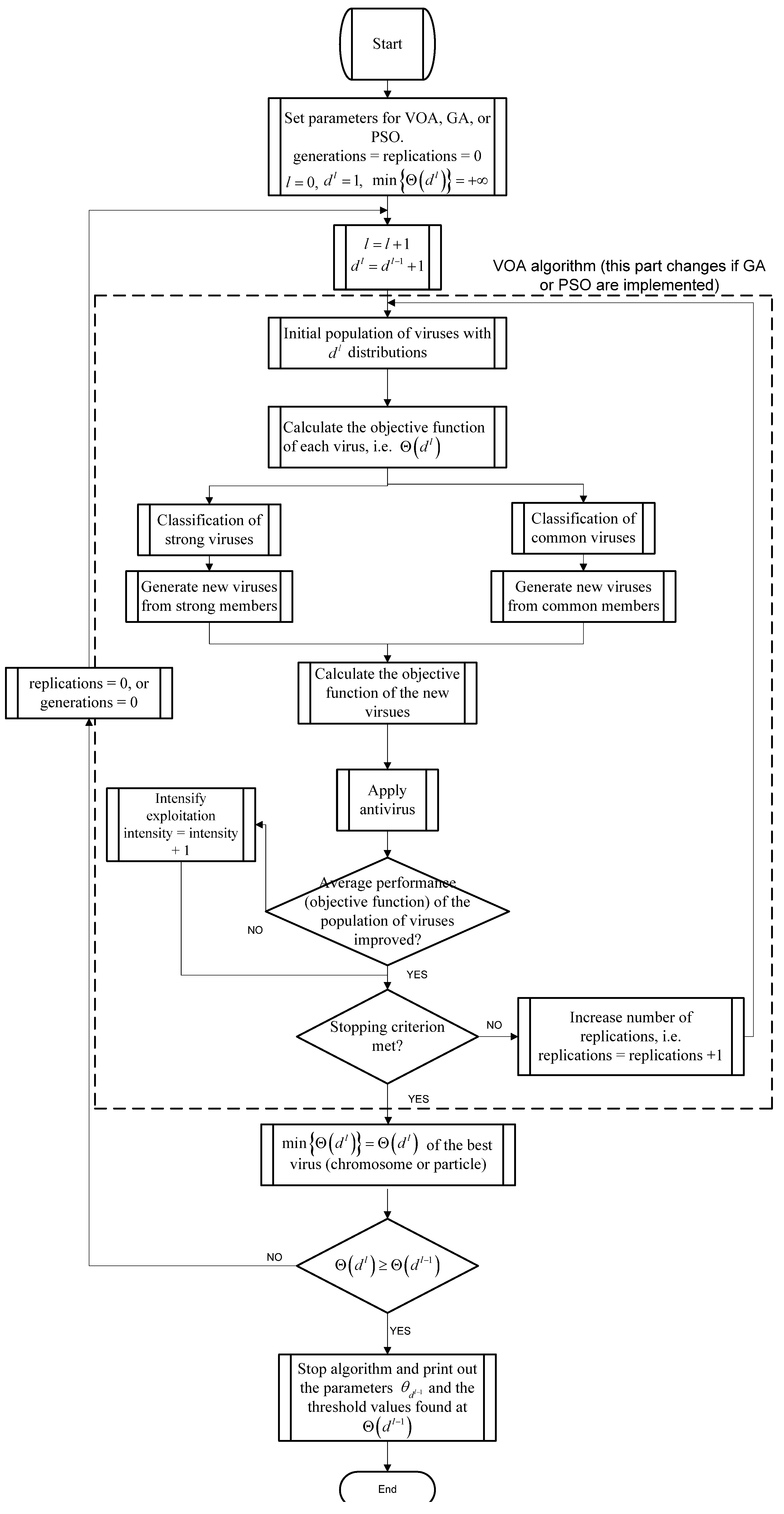
The basic idea of the DoE is to run the 34, 33, and 34, parameters combinations for VOA, GA, and PSO respectively, to later select which level (value) yielded the best performance (lower objective function value). Once the values for each parameter which delivered the best objective function value are identified, each test image is segmented by optimizing Equation (10) with each of the algorithmic tools used in this study.
The advantage of using DoE is that it is a systematic as well as well-known approach when deciding the setting yielding the best possible performance among all the combinations used during the full factorial design. In addition to the aforementioned, it is also a testing method that has been proven to be quite useful in many different areas such as tuning algorithm parameters [20].

3.2. Segmentation Results for the Proposed Model Using Meta-Heuristics as Optimization Tools

A comprehensive study of the proposed model implementing the three meta-heuristics introduced above is detailed in this part of Section 3. Additionally, a well-known segmentation method (Otsu’s) is implemented, where only the output image is observed in order to verify if the segmentation result given by the optimization algorithms used to minimize Equation (10) is as good as the one provided by Otsu’s method. The reason of the above mentioned, is because in terms of CPU time Otsu’s is a kind of exhaustive search approach; therefore, it is unfair to compare both ideas (the proposed approach and the Otsu’s method) in terms of computational effort.
Table 4, Table 5, Table 6, Table 7 and Table 8 detail the performance of the methods used for optimizing Equation (10) over different images. The results (objective function, threshold values, means, variances, and weights) are averaged over 50 independent runs, where the standard deviations of those 50 runs are not shown because they are in the order of 10−17.
By testing the image in Figure 4a it is observed that implementing the three meta-heuristics previously introduced for the optimization of Equation (10), the correct number of thresholds needed for segmenting the image is achieved (which is three). The computational effort and parameters of each Gaussian distribution ( θ j = { w j , μ j , σ j 2 } ) are summarized in Table 4. Here, the number of iterations for the algorithms were four, i.e., the proposed method optimized By testing the image in Figure 4a it is observed that implementing the three meta-heuristics previously introduced for the optimization of Equation (10), the correct number of thresholds needed for segmenting the image is achieved (which is 3).
Table 4. Thresholding results over 50 runs for the test image 1.
AlgorithmNumber of ThresholdsObjective FunctionThreshold ValuesMeansVariancesWeightsCPU Time per Iteration (s)Total CPU Time for the Proposed Approach (s)
VOA12.41024466.8083836.2120.6370.0260.507
251.39137.7090.363
20.97662, 24433.20912.8920.4830.071
175.8491298.0190.167
252.4520.6160.350
30.82644, 145, 24633.12311.2720.4800.117
78.128390.0790.021
187.900186.9870.149
252.4690.4820.350
40.89655, 97, 163, 24633.17812.1230.4820.294
75.522119.9100.017
128.441258.1190.003
185.92282.9200.142
252.1586.1770.356
GA12.41024469.8384226.0480.6500.1060.658
252.4520.6160.350
20.99465, 24233.23913.8060.4830.147
176.0181256.1420.166
252.4400.7360.351
30.85745, 111, 24233.13111.3500.4810.195
74.412187.0270.019
186.725207.5430.150
252.4400.7360.351
40.88244, 143, 155, 24733.12311.2720.4800.211
77.924377.9660.021
150.01312.3870.001
188.193191.8850.149
252.4770.4310.349
PSO12.38424770.1584274.1850.6510.0830.584
252.4770.4310.349
20.95565, 24733.23913.8060.4830.118
176.6721288.4210.167
252.4770.4310.349
30.85745, 111, 24233.13111.3500.4810.172
74.412187.0270.019
186.725207.5430.150
252.4400.7360.351
40.88042, 135, 154, 24733.09711.0700.4790.211
74.922381.8170.022
144.53535.0010.001
188.161192.7780.149
252.4770.4310.349
The computational effort and parameters of each Gaussian distribution ( θ j = { w j , μ j , σ j 2 } ) are summarized in Table 4. Here, the number of iterations for the algorithms were 4, i.e., the proposed method optimized Equation (10) for d = [1, 2, 3, 4] before reaching the stopping criterion.
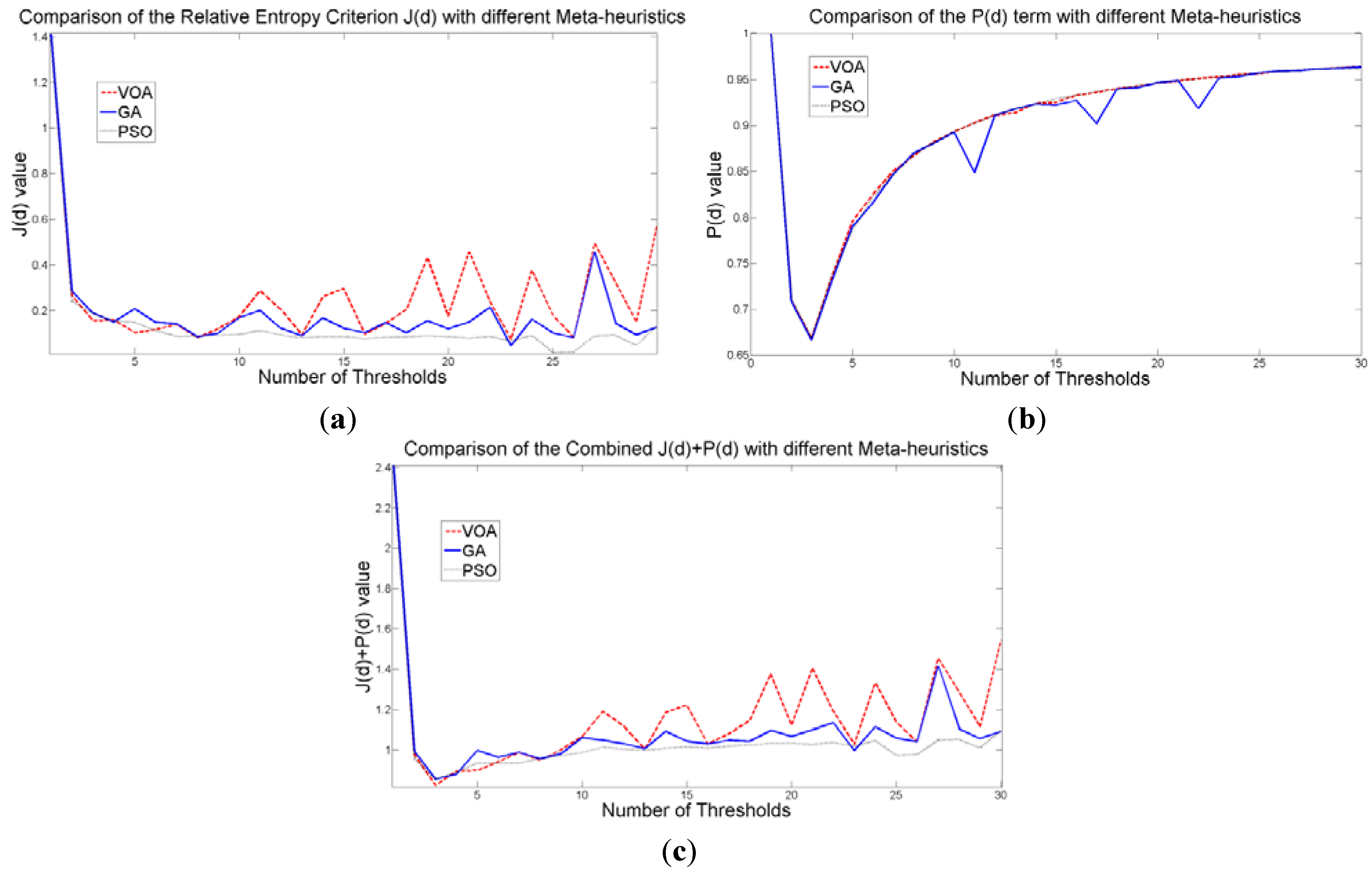
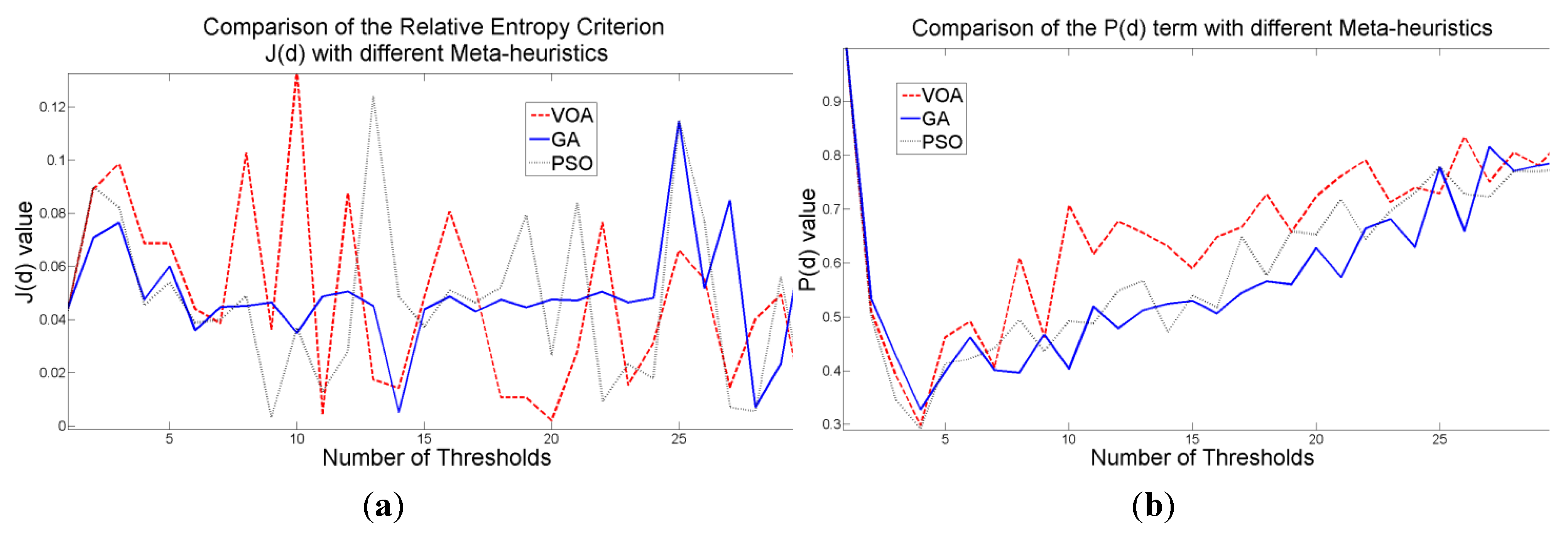
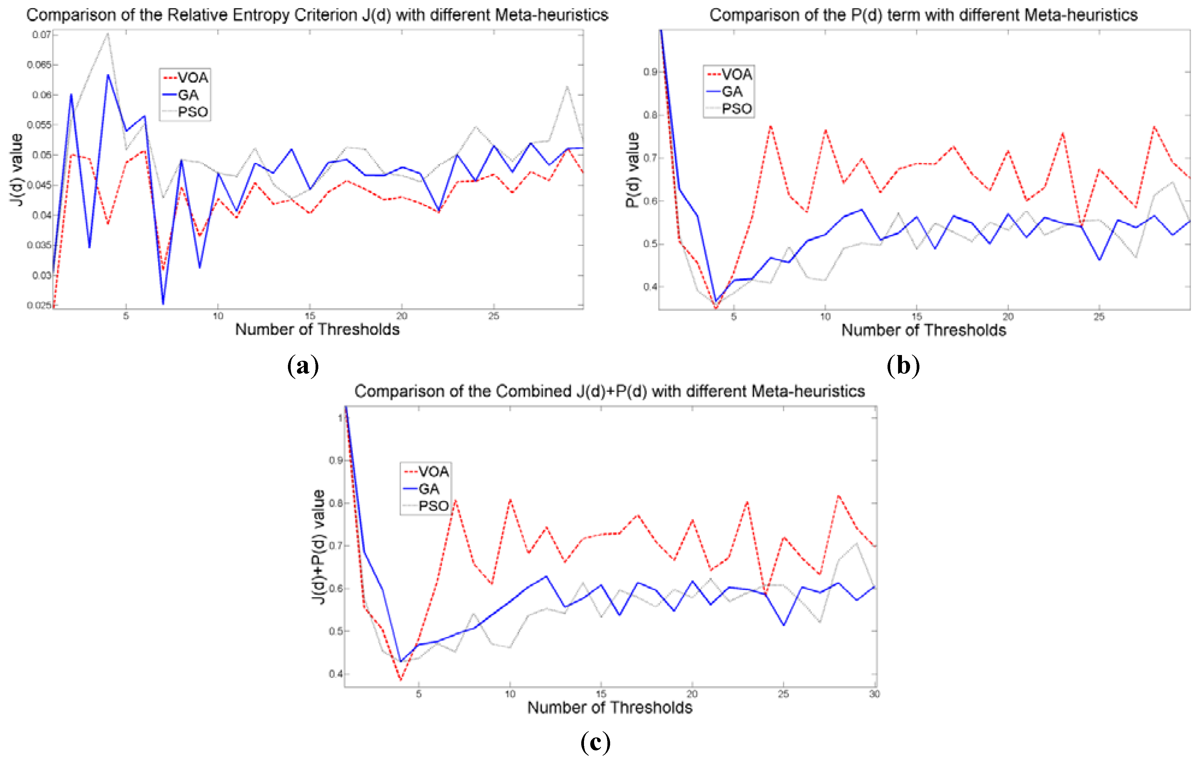
The behavior of the Relative Entropy function (Figure 7a) reveals its deficiency in detecting an appropriate number of distributions that will have a good description of the image histogram (Figure 8). The aforementioned is because as more distributions or thresholds are added into the mixture, it is impossible to identify a true minimum for the value of J(d) when implementing the three different meta-heuristic tools.
The additional function P(d) on the other hand shows a minimum value when a suitable number of distributions (which is the same as finding the number of thresholds) is found (
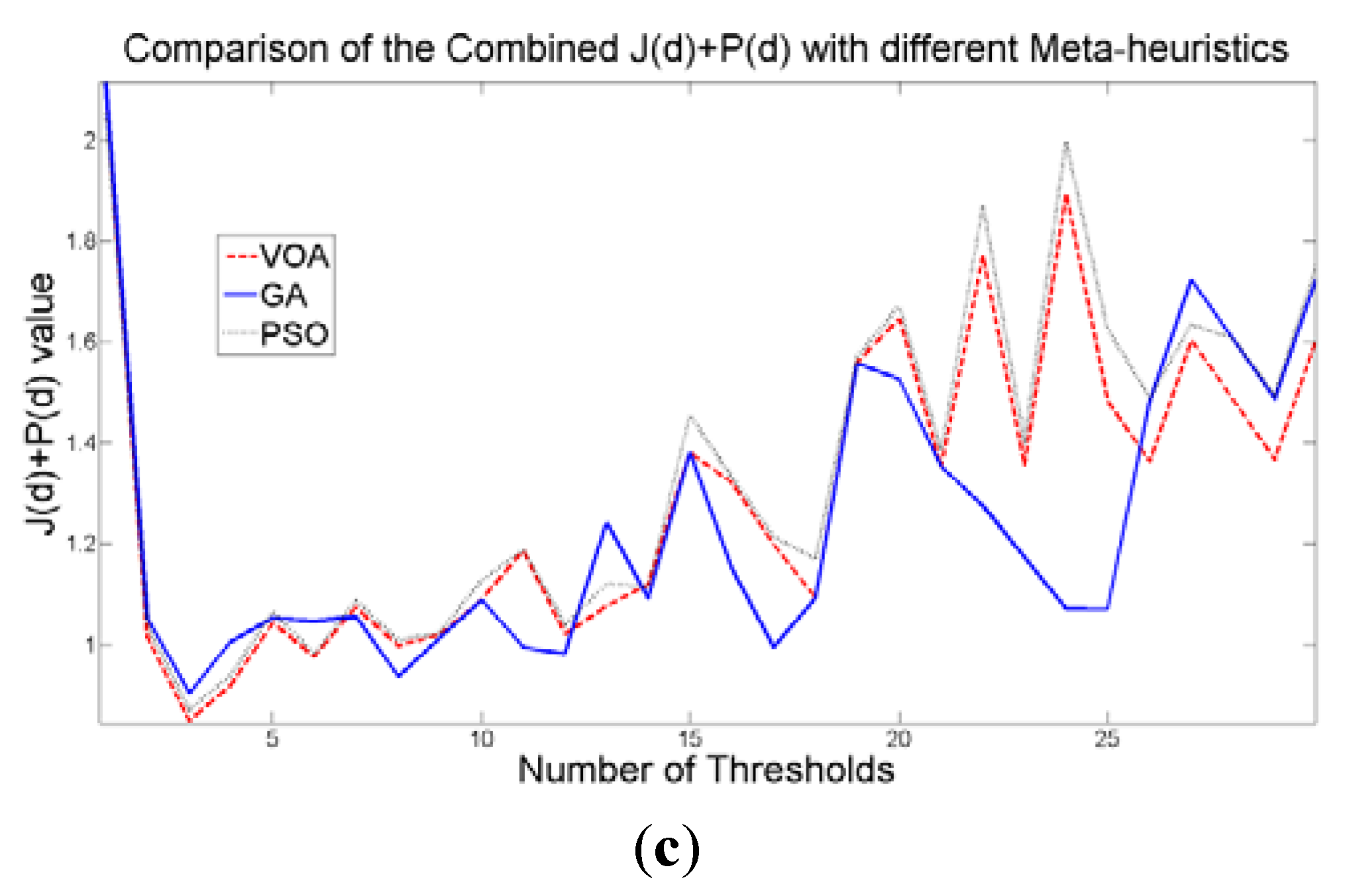
Figure 7b), since its value shows an increasing pattern when more distributions are added to the mixture model. The combination of these two functions J(d) and P(d) shows that the optimal value for Θ(d) (Figure 7c) will be when the number of thresholds is three as P(
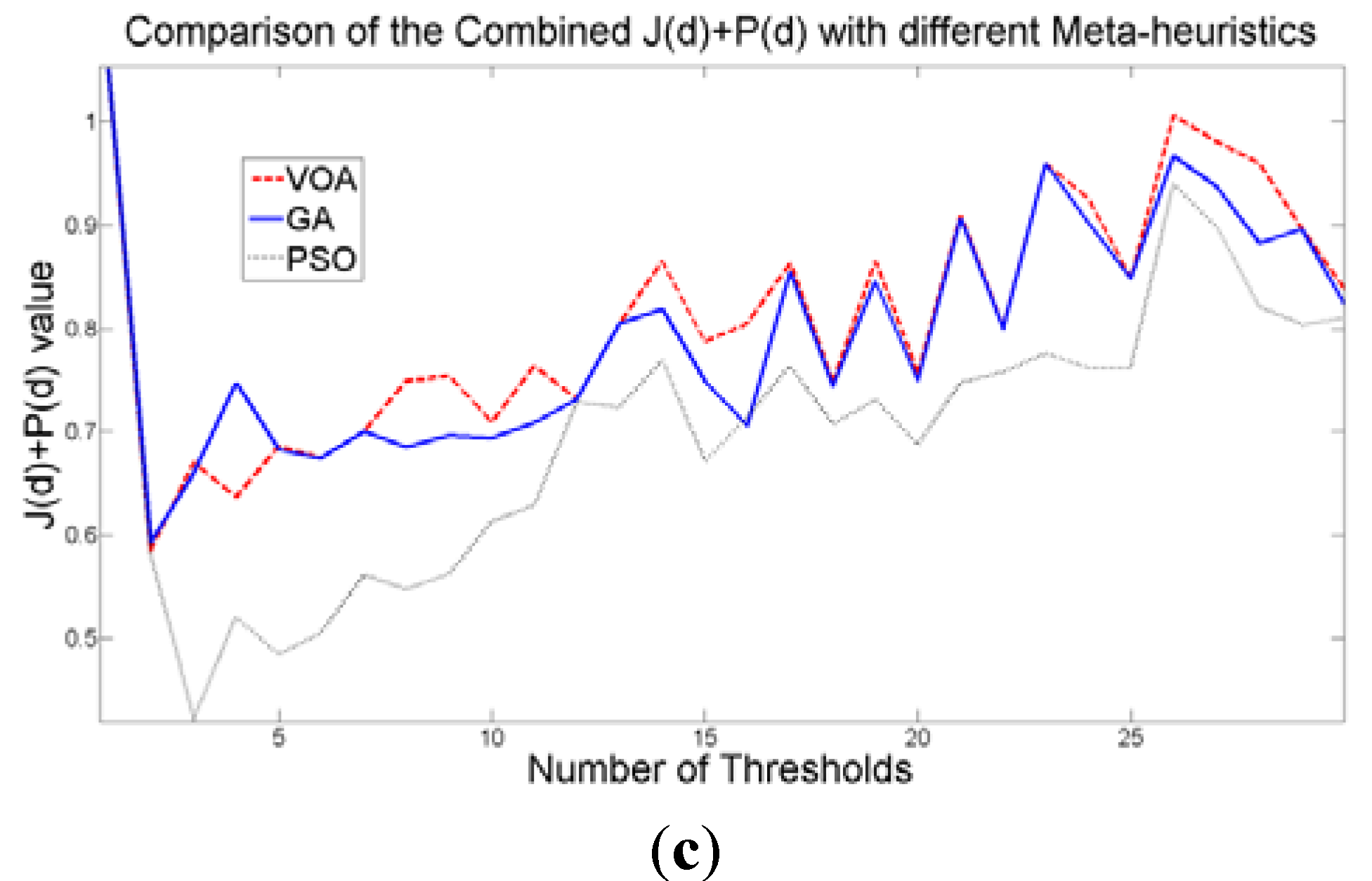
d) suggested. Note that the purpose of
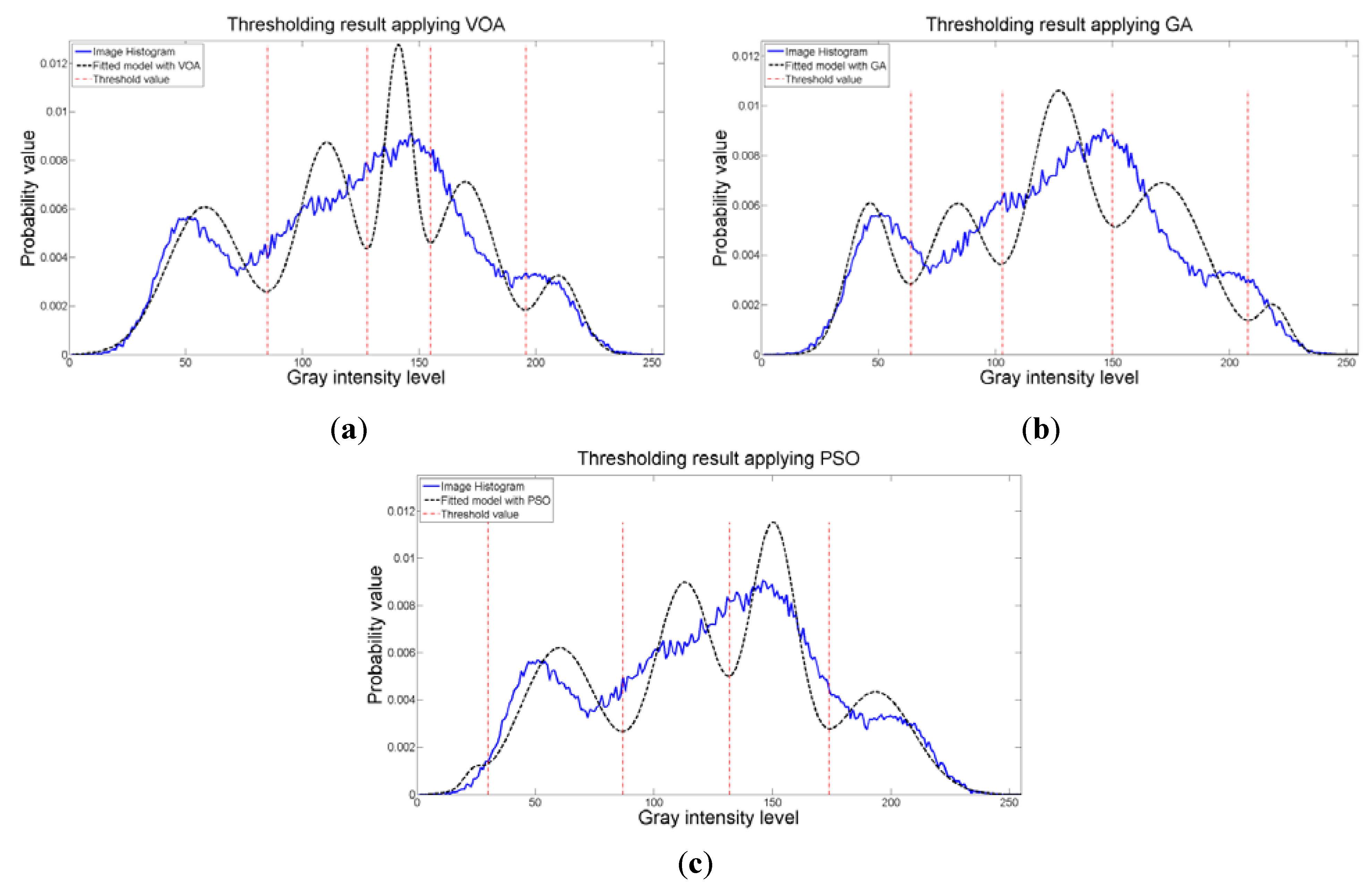
 J(d) is to find the best possible fitting with the suitable number of distributions (thresholds), and this is observed at 
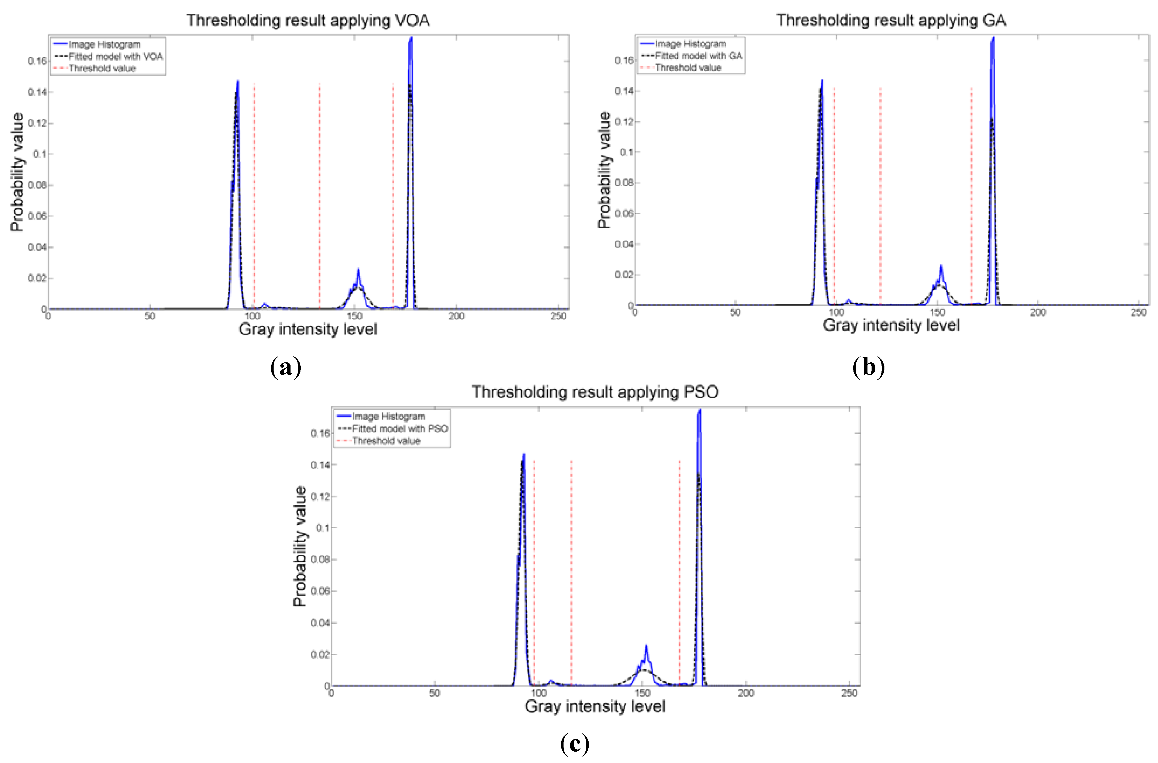
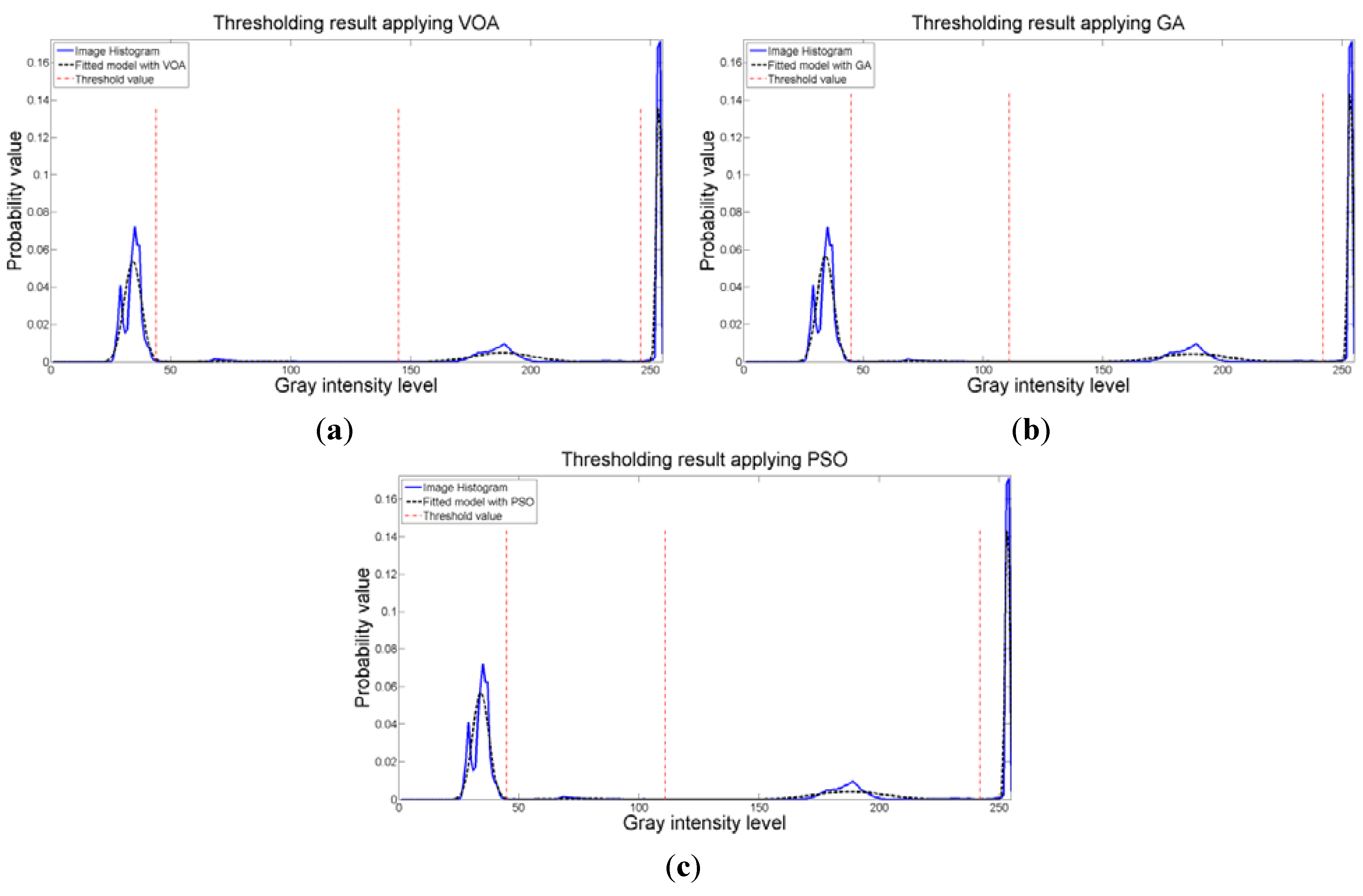
Figure 8 where the fitted model (dotted line) provides a very good description of the original histogram (solid line) given by the image. The vertical dashed lines in Figure 8 are the values of the threshold found. In addition to the thresholding result, it was observed that VOA provides both, the smallest CPU time as well as the best objective function value among the three algorithms.
Figure 7. Behavior of (a) Relative Entropy function J(d), (b) P(d), and (c) Objective function Θ(d) over different numbers of thresholds with different meta-heuristics VOA, GA and PSO on test image 1.
Entropy 15 02181 g007
Figure 8. Fitting of the histogram of the test image 1 implementing (a) VOA, (b) GA, and (c) PSO.
Entropy 15 02181 g008
When implementing Otsu’s method, it is rather impressive to observe that the output image delivered by the algorithms when optimizing Equation (10) resembles the one given by Otsu’s method (Figure 4e). The aforementioned, confirms the competitiveness of the proposed idea in segmenting a gray scale image given a number of distributions in the mixture model. Additionally, the main contribution is that we do not need to look at the histogram to determine how many thresholds will provide a good segmentation, and by implementing optimization tools such as the ones presented in this study, we can provide satisfactory results in a short period of time, where methods such as Otsu’s would take too long.
Table 5. Thresholding results over 50 runs for the test image 2.
AlgorithmNumber of ThresholdsObjective FunctionThreshold ValuesMeansVariancesWeightsCPU Time per Iteration (s)Total CPU Time for the Proposed Approach (s)
VOA11.05114387.3261015.9010.1270.0570.237
203.855603.4620.873
20.585133, 20581.590808.0540.1140.089
182.352280.5860.448
223.915170.1290.438
30.670104, 174, 20967.393370.0070.0820.091
150.866385.4860.153
192.99490.7750.378
226.231146.6020.386
GA11.05114286.658991.3360.1260.1090.480
203.746609.1170.874
20.593132, 20481.075790.0760.1130.145
181.537279.9920.436
223.310176.6420.451
30.659142, 149, 20686.658991.3360.1260.226
145.1213.9890.011
185.213205.9480.440
224.558163.3320.423
PSO11.05114387.3261015.9010.1270.0720.453
203.855603.4620.873
20.573156, 20697.7511389.4140.1530.141
186.458170.7890.424
224.558163.3320.423
30.619101, 180, 21166.048335.9440.0790.240
155.144453.1460.195
195.93276.3370.366
227.489134.9420.359
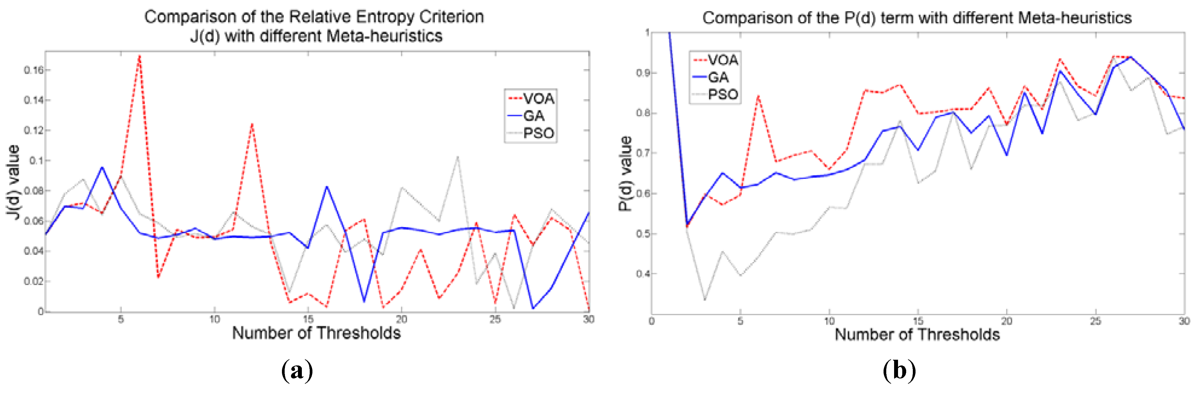
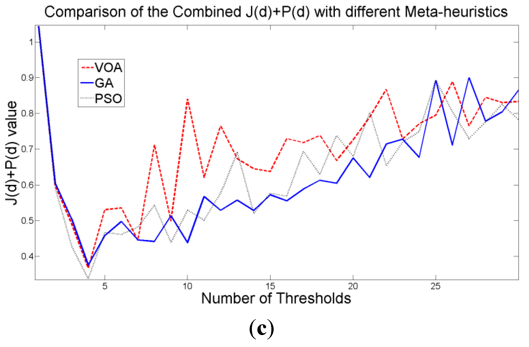
When an image containing text on a wrinkled paper (Figure 5a) is tested, two thresholds (or three Gaussian distributions) give the best objective function value for Equation (10) as observed in Figure 9c. Table 5 summarizes the thresholding results, i.e., Θ(d), computational effort and Gaussian parameters, for the three meta-heuristics implemented. As for the fitting result, Figure 10 shows that even though three Gaussian distributions do not provide an exact description of the image histogram, it is good enough to recognize all the characters on the thresholded image (Figure 5b–d).
Figure 9. Behavior of (a) Relative Entropy function J(d), (b) P(d), and (c) Objective function Θ(d) over different numbers of thresholds with different meta-heuristics VOA, GA and PSO on test image 2.
Entropy 15 02181 g009aEntropy 15 02181 g009b
The outstanding performance of the three meta-heuristics is observed once again when comparing with the Otsu’s method (Figure 5e), where the computational effort shows the feasibility of optimizing the proposed mathematical model with heuristic optimization algorithms.
Figure 10. Fitting of the histogram of the test image 2 implementing (a) VOA, (b) GA, and (c) PSO.
Entropy 15 02181 g010
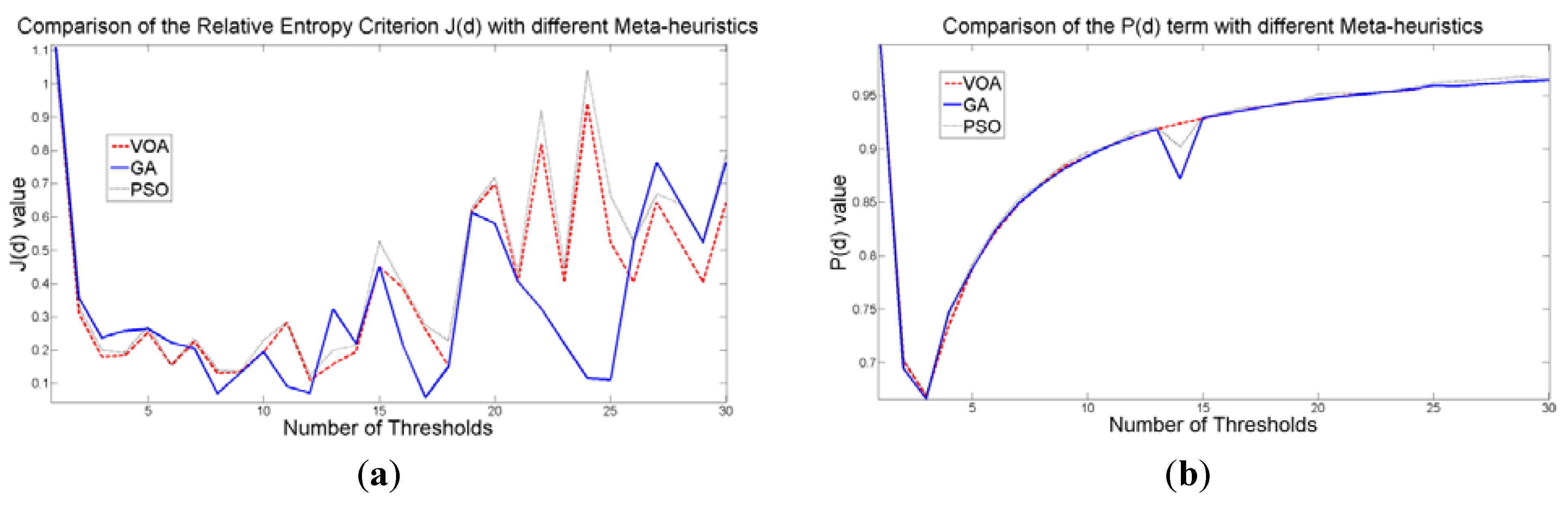
The thresholding results of the Lena image (Figure 6a) shows that four thresholds (five Gaussian distributions) have the best objective function value, which is detailed in Table 6. Visually, the thresholded images (Figure 6b–d) obtain most of the details from the original one, and in terms of objective function behavior (Figure 11) there is no need to add more distributions into the mixture model (i.e., more thresholds) because they do not provide a better objective function value.
Table 6. Thresholding results over 50 runs for the test image 3.
AlgorithmNumber of ThresholdsObjective FunctionThreshold ValuesMeansVariancesWeightsCPU Time per Iteration (s)Total CPU Time for the Proposed Approach (s)
VOA11.0436348.91751.3980.1590.0461.009
138.0481442.0950.841
20.57559, 13847.59840.1000.1430.128
104.785484.3610.430
168.523538.2130.428
30.45499, 140, 18365.002369.2330.3020.198
120.137147.6210.287
157.234130.1550.295
201.595109.6460.116
40.36786, 126, 154, 19957.243192.4330.2360.210
106.550126.9380.236
139.62967.6660.241
170.694173.7330.218
208.85142.4590.068
50.46668, 104, 134, 156, 19050.38068.1880.1750.428
88.813108.6220.165
120.05477.6560.203
145.07239.8450.192
168.59790.4000.167
204.36477.7220.098
GA11.0446649.79460.8740.1690.1030.904
138.9241393.4560.831
20.60669, 13950.67172.0950.1780.136
109.090368.0750.402
169.106530.3580.419
30.50496, 140, 17962.664315.8260.2820.182
118.590171.1800.307
156.168110.2430.282
199.453139.5100.129
40.47446, 99, 136, 16940.69814.5830.0510.225
69.954296.6230.251
118.032124.1290.256
151.05377.6030.267
192.624235.7360.175
50.58465, 87, 128, 152, 20549.50457.5500.1660.258
76.02340.4150.074
108.258138.2920.250
139.53349.5220.205
171.707244.6130.257
211.82428.0180.049
PSO11.0446449.21254.3870.1630.0960.887
138.3531424.9780.837
20.57568, 14050.38068.1880.1750.128
109.403387.9840.414
169.718522.3300.411
30.44697, 141, 19163.440333.7410.2880.170
119.639170.1990.309
159.625168.7840.308
204.79073.7280.095
40.33779, 121, 148, 18454.216131.1790.2100.220
101.036126.5410.225
134.32760.4740.225
161.86695.3550.227
202.037103.8440.113
50.47860, 115, 117, 147, 18647.92642.5820.1470.273
90.827237.6790.255
115.5140.2500.010
132.32271.3310.240
161.755107.9860.240
202.78294.6390.108
Figure 11. Behavior of (a) Relative Entropy function J(d), (b) P(d), and (c) Objective function Θ(d) over different numbers of thresholds with different meta-heuristics VOA, GA and PSO on test image 3.
Entropy 15 02181 g011aEntropy 15 02181 g011b
Once again, the fitting provided by the mixture model (Figure 12) might not be the best; however, it is good enough to provide most of the details from the original image. It is interesting to observe that all the algorithmic tools are able to find satisfactory results in no more than 1.009 seconds in the case of VOA which is the slowest one, even though the algorithmic tools had to optimize Equation (10) for d = [1, 2, 3, 4].
Figure 12. Fitting of the histogram of the test image 3 implementing (a) VOA, (b) GA, and (c) PSO.
Entropy 15 02181 g012
To further test the proposed method an image with low contrast is used as illustrated in Figure 13a. It is observed that all the algorithmic tools are able to segment the image providing the correct number of thresholds which is three. Additionally, when comparing the output image given by Otsu’s method and the idea proposed in this study, we are able to observe that despite its novelty the proposed method provides stable and satisfactory results for a low contrast image.
Three thresholds are suggested after the optimization of Equation (10) is performed, which is good enough for successfully segmenting the image under study (Figure 13b–d), though the fitting of the image histogram was not a perfect one (Figure 15). More importantly, the addition of more than four distributions (i.e., three thresholds) to the mathematical model Equation (10) does not achieve a better result according to Figure 14c; therefore, the power of the proposed approach is shown once again with this instance. As for the Otsu’s method, even though the correct number of thresholds is provided, the low contrast causes defect in the output image (seen at the light gray region in the middle of Figure 13e.
Table 7. Thresholding result over 50 runs for the test image 4.
AlgorithmNumber of ThresholdsObjective FunctionThreshold ValuesMeansVariancesWeightsCPU Time per Iteration (s)Total CPU Time for the Proposed Approach (s)
VOA12.11298102.027504.5950.6120.0450.213
174.62236.1650.388
21.014105, 16991.0072.9940.4860.051
146.853157.4620.160
176.4150.7490.354
30.848101, 133, 16990.9171.8880.4820.054
109.43846.6370.019
150.66717.2580.145
176.4150.7490.354
40.919103, 117, 140, 16990.9292.0090.4830.064
107.79617.8530.016
126.81825.7140.002
150.2029.1410.139
176.2712.3260.359
GA12.1129890.9061.8030.4820.1340.692
166.703268.2340.518
21.051100, 16690.9141.8610.4820.153
145.534191.6240.161
176.3491.3540.357
30.90399, 122, 16790.9101.8320.4820.179
107.75923.6400.018
150.17119.4520.144
176.3641.2030.356
40.998109, 115, 139, 17791.2706.8290.4940.225
111.8492.5750.003
123.65552.3050.005
164.654163.3350.323
177.0001.4550.176
PSO12.1129890.9061.8030.4820.0270.171
166.703268.2340.518
21.00597, 16890.9021.7800.4810.035
145.505204.5820.163
176.3930.9310.355
30.87398, 116, 16890.9061.8030.4820.045
106.39312.9560.016
149.89933.9450.147
176.3930.9310.355
40.91198, 130, 138, 16990.9061.8030.4820.065
108.77742.8330.019
133.1104.1220.001
150.70416.7070.144
176.4150.7490.354
Figure 13. 
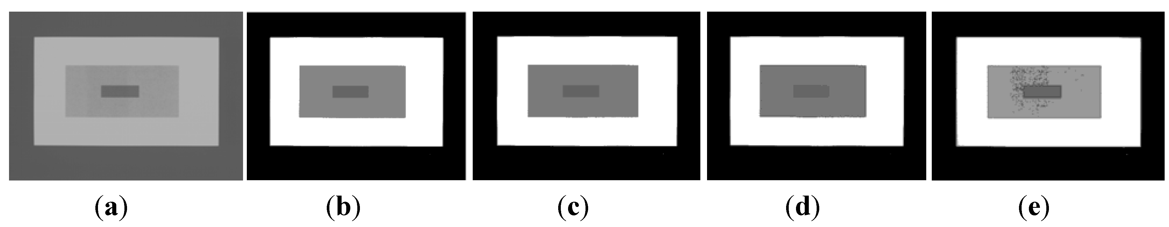
Test image 4: (a) Original image; Thresholded image implementing (b) VOA, (c) GA, (d) PSO, and (e) Otsu’s method.
Entropy 15 02181 g013
Figure 14. Behavior of (a) Relative Entropy function J(d), (b) P(d), and (c) Objective function Θ(d) over different numbers of thresholds with different meta-heuristics VOA, GA, and PSO on test image 4.
Entropy 15 02181 g014aEntropy 15 02181 g014b
Figure 15. Fitting of the histogram of the test image 4 implementing (a) VOA, (b) GA, and (c) PSO.
Entropy 15 02181 g015
Table 8. Thresholding result over 50 runs for the test image 5.
AlgorithmNumber of ThresholdsObjective FunctionThreshold ValuesMeansVariancesWeightsCPU Time per Iteration (s)Total CPU Time for the Proposed Approach (s)
VOA11.0236748.328119.0830.1720.0600.435
138.3011428.5550.828
20.55663, 13746.555100.2920.1550.075
104.962436.4100.421
168.426564.1540.424
30.50488, 140, 20657.730278.2080.2540.082
115.780221.2870.346
165.005334.7900.358
214.73550.9560.042
40.48187, 130, 151, 19757.218267.8320.2490.094
109.591151.0590.268
140.15336.6190.178
168.811169.3020.232
209.13878.8200.071
50.49577, 116, 143, 158, 214, 25552.347176.7100.2080.124
97.798120.0790.210
129.63659.4640.208
149.84218.4710.128
180.649270.3080.226
220.58134.8730.020
GA11.0247149.927139.3170.1870.1391.204
139.5771363.8790.813
20.66976, 13751.913169.4990.2040.198
109.784294.4140.372
168.426564.1540.424
30.58684, 138, 22755.674237.2430.2360.209
113.180235.4100.347
168.529529.9080.413
231.26120.7820.003
40.56860, 103, 146, 21145.13887.6330.1410.259
82.720165.6070.195
125.553152.1880.316
170.644343.1070.320
218.25340.3080.028
50.57357, 90, 130, 156, 21243.63576.3010.1260.400
72.88199.7720.138
110.800131.9730.254
142.59055.3910.220
178.408270.8370.237
219.03538.3680.025
PSO11.0236647.900114.2200.1680.0340.373
137.9481446.9830.832
20.56464, 13747.023104.9220.1590.060
105.419421.7510.416
168.426564.1540.424
30.41397, 140, 18263.047390.7060.3000.073
119.448154.2170.300
157.206130.6060.281
201.012152.7730.119
40.41028, 89, 133, 16922.82517.0560.0070.091
59.246263.4070.252
112.179160.0430.284
149.44199.4320.282
192.596259.8380.175
50.57640, 70, 125, 159, 23032.58032.7140.0370.115
53.83068.5460.146
100.401235.2020.297
141.67192.6910.281
184.398346.0420.237
234.12219.7970.002
The Lena image in which a random noise is generated will be our last test instance (Figure 16a), from this it is expected to provide clear evidence concerning robustness of the proposed method, where all the parameter values and computational results are summarized on Table 8. By observing the thresholded images when implementing the proposed approach (Figure 16b–d), we are able to conclude that random noise does not represent a major issue, even though different optimization tools are used.
The objective function behavior (Figure 17c) proved once again that when a suitable number of thresholds is achieved, the addition of more distributions into the mixture model is not necessary, since it will always achieve a larger objective function value compared with the one given by having four thresholds (or five Gaussians). Additionally, the fitting of the histogram (Figure 18) given by the image, even though is not a perfect one, is proved to be good enough to keep most of the relevant details from the original test instance.
Most of the relevant details from the original instance are kept. On the other hand, Otsu’s method (Figure 16e) is not able to provide an output image as clear as the ones given by the proposed approach when implementing the meta-heuristic tools.
Figure 16. Test image 5: (a) Original image; Thresholded image implementing (b) VOA, (c) GA, (d) PSO, and (e) Otsu’s method with 4 thresholds.
Entropy 15 02181 g016
Figure 17. Behavior of (a) Relative Entropy function J(d), (b) P(d), and (c) Objective function Θ(d) over different numbers of thresholds with different meta-heuristics VOA, GA and PSO on test image 5.
Entropy 15 02181 g017
Figure 18. Fitting of the histogram of the test image 5 implementing (a) VOA, (b) GA, and (c) PSO.
Entropy 15 02181 g018

4. Conclusions

In this study a new approach to automatically assess the number of components “d” in a mixture of Gaussians distributions has been introduced. The proposed method is based on the Relative Entropy Criterion (Kullback-Leibler information distance) where an additional term is added to the function and helps to determine a suitable number of distributions. Finding the appropriate number of distributions is the same as determining the number of thresholds for segmenting an image, and this study has further shown that the method proposed in [8] is powerful enough in finding a suitable number of distributions (thresholds) in a short period of time.
The novelty of the approach is that, not only an appropriate number of distributions determined by P(d) is achieved, but also a good fitting of the image histogram is obtained by the Relative Entropy function J(d). The optimization of Equation (10) was performed implementing the Virus Optimization Algorithm, Genetic Algorithm, Particle Swarm Optimization, and the output images are compared to that given by a well-known segmentation approach Otsu’s method. The objective function behavior shows that the proposed model achieves a suitable number of thresholds when its minimum value is achieved, and the addition of more distributions (thresholds) into the model will cause an increasing trend of the model in Equation (10).
Comparing the proposed method with Otsu’s method provided clear evidence of the effectiveness and efficiency of the approach where the algorithmic tools are used in order to reduce the computational effort when optimizing Equation (10). Additionally, the proposed method proved to reach the same value for the number of thresholds needed for the segmentation of the images tested in this study, even though different optimization algorithms were implemented.
It is worth mentioning that the proposed method proved to work remarkably well under test images with low contrast and random noise. A suitable number of thresholds and an outstanding result in the output thresholded images were obtained. Whereas for the Otsu’s method, the output image showed some defects once the segmentation was performed.
The fitting result coming from the proposed approach might not be the best; however, when segmenting an image what matters the most is the fidelity in which most of the details are kept from the original picture. This is what makes the difference between a good and poor segmentation result. Future directions point toward testing the proposed method with more meta-heuristic algorithms, as well as a wider range of images to evaluate the robustness of the approach.

Acknowledgments

This work was partially supported by National Science Council in Taiwan (NSC-100-2628-E-155-004-MY3).

References

  1. Shapiro, L.G.; Stockman, C. Computer Vision; Prentice Hall: Upper Saddle River, NJ, USA, 2002. [Google Scholar]
  2. Jiao, L.C.; Gong, M.G.; Wang, S.; Hou, B.; Zheng, Z.; Wu, Q.D. Natural and remote sensing image segmentation using memetic computing. IEEE Comput. Intell. Mag. 2010, 5, 78–91. [Google Scholar] [CrossRef]
  3. Zhang, H.; Fritts, J.E.; Goldman, S.A. Image segmentation evaluation: A survey of unsupervised methods. Comput. Vis. Image Underst. 2008, 110, 260–280. [Google Scholar] [CrossRef]
  4. Ashburner, J.; Friston, K.L. Image Segmentation. In Human Brain Function, 2nd. ed.; Academic Press: Waltham, MA, USA, 2004; Chapter 35; pp. 695–706. (free version of the chapter can be found at: http://www.fil.ion.ucl.ac.uk/spm/doc/books/hbf2/pdfs/Ch5.pdf).
  5. Qin, K.; Li, D.; Wu, T.; Liu, Y.C.; Chen, G.S.; Cao, B.H. A comparative study of type-2 fuzzy sets and cloud model. Int. J. Comput. Intell. Syst. 2010, 3, 61–73. [Google Scholar]
  6. Glover, F.K. Handbook of Metaheuristics; Springer: New York, NY, USA, 2003. [Google Scholar]
  7. Safabakhsh, R.; Hosseini, H.S. Automatic multilevel thresholding for image segmentation by the growing time adaptive self-organizing map. IEEE Trans. Pattern Anal. Mach. Intell. 2002, 24, 1388–1393. [Google Scholar]
  8. Liang, Y.C.; Cuevas, J.R. Multilevel image thresholding using relative entropy and virus optimization algorithm. In Proceedings of the 2012 IEEE World Congress on Computational Intelligence (WCCI2012), Brisbane, Australia, 10–15 June 2012; pp. 1–8.
  9. Kullback, S.; Leibler, R.A. On information and sufficiency. Ann. Math. Stat. 1951, 22, 79–86. [Google Scholar] [CrossRef]
  10. McLachlan, G.; Peel, D. Finite Mixture Models; John Wiley & Sons: Hoboken, NJ, USA, 2001. [Google Scholar]
  11. Rice, J. Mathematical Statistics and Data Analysis, 2nd ed.; Duxbury Press: Pacific Grove, CA, USA, 1995. [Google Scholar]
  12. Arora, S.; Acharya, K.; Verma, A.; Panigrahi, P.K. Multilevel thresholding for image segmentation through a fast statistical recursive algorithm. Pattern Recogn. Lett. 2006, 29, 119–125. [Google Scholar] [CrossRef]
  13. Chao, R.M.; Wu, H.C.; Chen, Z.C. Image segmentation by automatic histogram thresholding. In Proceedings of the 2nd International Conference on Interaction Sciences: Information Technology, Culture and Human, Seoul, Korea, 24–26 November 2009; pp. 136–141.
  14. Hammouche, K.; Diaf, M.; Siarry, P. A comparative study of various meta-heuristic techniques applied to the multilevel thresholding problem. Eng. Appl. Artif. Intel. 2010, 23, 676–688. [Google Scholar] [CrossRef]
  15. Yen, J.C.; Chang, F.J.; Chang, S. A new criterion for automatic multilevel thresholding. IEEE Trans. Image Process. 1995, 4, 370–378. [Google Scholar] [PubMed]
  16. Wang, H.J.; Cuevas, J.R.; Lai, Y.C.; Liang, Y.C. Virus Optimization Algorithm (VOA): A novel metaheuristic for solving continuous optimization problems. In Proceedings of 10th Asia Pacific Industrial Engineering & Management System Conference (APIEMS), Kitakyushu, Japan, 14–16 December 2009; pp. 2166–2174.
  17. Holland, J.H. Adaptation in Neural and Artificial Systems; University of Michigan Press: Ann Arbor, MI, USA, 1975. [Google Scholar]
  18. Kennedy, J.; Eberhart, R. Particle swarm optimization. In Proceedings of IEEE International Conference on Neural Networks, Perth, Australia, 27 November–1 December 1995; pp. 1942–1948.
  19. Box, G.E.; Hunter, W.G.; Hunter, J.S. Statistics for Experimenters: Design, Innovation, and Discovery; John Wiley & Sons: New York, NY, USA, 2005. [Google Scholar]
  20. Myers, R.H.; Montgomery, D.C.; Cook, C.M. Response Surface Methodology: Process and Product Optimization Using Designed Experiments, 3rd ed.; Wiley Series in Probability and Statistics; John Wiley & Sons: Hoboken, NJ, USA, 2009. [Google Scholar]

