Vessel Pattern Knowledge Discovery from AIS Data: A Framework for Anomaly Detection and Route Prediction

Abstract

Understanding maritime traffic patterns is key to Maritime Situational Awareness applications, in particular, to classify and predict activities. Facilitated by the recent build-up of terrestrial networks and satellite constellations of Automatic Identification System (AIS) receivers, ship movement information is becoming increasingly available, both in coastal areas and open waters. The resulting amount of information is increasingly overwhelming to human operators, requiring the aid of automatic processing to synthesize the behaviors of interest in a clear and effective way. Although AIS data are only legally required for larger vessels, their use is growing, and they can be effectively used to infer different levels of contextual information, from the characterization of ports and off-shore platforms to spatial and temporal distributions of routes. An unsupervised and incremental learning approach to the extraction of maritime movement patterns is presented here to convert from raw data to information supporting decisions. This is a basis for automatically detecting anomalies and projecting current trajectories and patterns into the future. The proposed methodology, called TREAD (Traffic Route Extraction and Anomaly Detection) was developed for different levels of intermittency (i.e., sensor coverage and performance), persistence (i.e., time lag between subsequent observations) and data sources (i.e., ground-based and space-based receivers).

1. Introduction

Maritime transportation represents approximately 90% of global trade by volume, placing safety and security challenges as a high priority for nations across the globe. Maritime surveillance data are collected at different scales and are increasingly used to achieve higher levels of situational awareness.

Automatic Identification System (AIS) technology provides a vast amount of near-real time information, calling for an ever increasing degree of automation in transforming data into meaningful information to support operational decision makers. As an example, the Centre for Maritime Research and Experimentation (CMRE) is currently receiving an average rate of 600 Million AIS messages per month from multiple sources, and the rate is increasing [1]. AIS is a self-reporting messaging system originally conceived for collision avoidance (AIS is mandatory for ships of 300 gross tonnage and upwards in international voyages, 500 and upwards for cargoes not in international waters and passenger vessels [2]. In addition, fishing vessels greater than 15 m sailing in water under the jurisdiction of the European Union Member States shall also be required to be fitted with AIS [3].) to broadcast information on their location (positional, identification and other information) at a variable refresh rate, which depends on their motion (vessels at anchor transmit their position every two minutes and increase the broadcast rate up to two seconds when maneuvering or sailing at high speed; every five minutes, vessels transmit other data (static and voyage related information) containing identifiers, such as International Maritime Organization (IMO) number, call sign, ship name and Maritime Mobile Service Identity (MMSI), used as a primary key to link the message to position information. Static information also includes size, type of vessel and cargo, whereas voyage related data, such as Estimated Time of Arrival (ETA) and destination, are manually set and not fully reliable [4].) Over the last several years, the AIS data received by ships and coastal stations have been transmitted to regional or national data centers. When multiple receivers are connected into networks, certain challenges arise with data intermittency, resolving data redundancy received by multiple receivers, correcting errors in timestamps assigned by varying receivers and identifying tracks of vessels that erroneously share the message identifier. This level of pre-processing is necessary to extract maritime motion patterns, especially at a global scale.

Receiving AIS messages from space [5] is becoming increasingly commonplace. As opposed to terrestrial networks of AIS receivers, whose performance is characterized by high persistence, but limited coverage, satellite-based systems can pick up messages in the open sea, far away from the coastline. Space-based receivers tend to be mounted on Low Earth Orbit (LEO) satellites, so the AIS coverage is global at the expense of persistence, due to the orbiting platform revisit time. It is clear that when integrating such systems with data received by terrestrial receivers, there are additional issues to resolve with variable frequency update, coverage and persistence.

In this work, a methodology is presented that aims to convert the large amount of AIS data into decision support elements, independently of the number of receivers, their performance, the platform of origin and the scale of the area of interest. The knowledge is extracted via an incremental learning approach, in order to dynamically adapt to evolving situations (e.g., maritime seasonal patterns, operational conditions or changing routing schemes). This allows maritime traffic to be characterized following a fully unsupervised learning strategy with no a priori information needed (i.e., using only raw AIS data).

The proposed traffic route extraction methodology can be used to provide up-to-date high level contextual information (e.g., Level 2 processing in the Joint Directors of Laboratories (JDL) model [6]). Knowledge of traffic routes is a useful input to situational awareness and helps in understanding seasonal variations in traffic patterns. Besides traffic densities, the extracted routes provide useful information on daily patterns and transit duration differentiated by vessel types. Further, extracted routes enable realistic simulations of traffic, which are useful to test and evaluate target tracking performance, the effectiveness of surveillance technologies and other decision support frameworks.

Generated contextual maritime knowledge can also be used to perform rule-based and low-likelihood anomaly detection. Rule-based anomaly detection approaches refer to the generation of alerts based on a set of rules [7], such as maximum speed allowed in a port, presence in areas restricted to navigation or inconsistencies between ship claimed and actual activity. Conversely, low-likelihood anomaly detection aims at detecting deviations from “normality” of vessel traffic patterns derived in the learning phase (see, e.g., [8] and references therein) and is illustrated via an example provided in the present work. Behaviors that differ from “normality” do not necessarily mean they are “anomalies” in an operational context, but they are highlighted as unusual for further analysis.

The vessel traffic and motion information, once extracted, can be alternatively exploited to perform ship route prediction at a given time. This is the process of predicting ship movements well beyond any available positioning data, based on behaviors of past vessels on the same route. This is useful, for example, in counter piracy applications to identify risk areas associated with the joint predicted presence of white shipping density (e.g., commercial merchant traffic) and Pirates Action Groups (PAG) [9]. Backward and forward tracking of vessels can also be significantly improved using the learned maritime traffic patterns, which are particularly useful when attempting to fuse AIS and space-based optical or Synthetic Aperture Radar (SAR) information (e.g., [10]).

The distribution and characterization of traffic can also be used for augmenting remote sensing tracking and classification performance, enabling knowledge-based tracking and classification (e.g., [11]). Specifically, the knowledge of vessel patterns can be used for (i) connecting tracks originated by the same target and broken by gaps in coverage or reduced observability and/or (ii) providing a priori knowledge about the vessel type for classification purposes.

In Section 2, we give a brief review of related work on traffic characterization and route knowledge extraction. We discuss the traffic knowledge discovery methodology in Section 3. This is followed by some examples of route knowledge exploitation in Section 4: the route classification is given in Section 4.1. Two specific applications (i.e., route prediction and anomaly detection) are provided in Section 4.2 and Section 4.3, respectively, to illustrate the potential of the derived knowledge. Finally, concluding remarks are given in Section 5.

2. Related Work

The application of statistical methodologies to derive motion patterns from a collection of trajectories in an unsupervised way is a challenging task. Several methods have been proposed as applied in video surveillance and image processing (e.g., [12,13,14,15,16]). In [17], a probabilistic model to track human behavior over time is presented. The papers [18,19,20,21] specifically deal with maritime applications, although using image processing techniques. Reference [12] presented an extensive model to statistically learn motion patterns without any prior knowledge in traffic scenes where the traffic flows are constrained to stay in specific areas. The application of such techniques in maritime situational awareness has gained an increasing acceptance during recent years. One possible approach is to subdivide the area of interest into a spatial grid whose cells are characterized by the motion properties of the crossing vessels (e.g., [10,22,23]). Although effective for small area surveillance, the main limitations of the “grid”-based approach resides in the required computational burden when increasing the scale, as well as the need for a priori selection of the optimal cell size. In areas characterized by complex traffic, like intersecting sea lanes, the resulting multi-modal behavioral description would lead to complex algorithms to perform anomaly detection. A new trend in the field of maritime anomaly detection is to adopt a “vectorial” representation of traffic, where trajectories are thought of as a set of straight paths connecting waypoints; this allows a compact representation of vessel motions that can be implemented at a global scale. In the works reported in [24,25], the waypoints are nodes in the proximity of land masses, and Great Circle routes are formed to represent ocean journeys. In areas characterized by complex routing systems, it is necessary to further introduce intermediate nodes (i.e., turning points) to more accurately describe routes. For [26,27], turning points are detected in areas where changes in the Course Over Ground (COG) of vessels are consistently observed. One of the limitations of “vectorial” approaches is the detection of turning points in unregulated areas, where the behavior of vessels is much more complex and, therefore, difficult to categorize. The present paper addresses this practical issue: the representation of maritime traffic is still “vectorial”, but in contrast to previous research, the route objects are directly formed by the flow vectors of the vessels whose paths connect the derived waypoints (i.e., stationary areas, as well as entry and exit points). Specifically, the approach introduced here is based on a preliminary clustering of waypoints. Trajectories are, then, identified between such waypoints. Differently from other “vectorial” representations, the route objects include directional changes without explicitly deriving turning points. As will be seen, it is still possible to consistently capture maritime patterns in a compact and accurate way. It is also feasible to extract temporal information, like route travel time distributions and daily patterns, as well as to associate historical route patterns to vessels. These features enable the discovery of maritime traffic knowledge that can be used to implement higher level anomaly detection tools. Additionally, the distance-based approach, adopted in [26,27], was not always effective in distinguishing waypoints close to each other. In order to overcome this difficulty, a density-based algorithm (i.e., DBSCAN—Density-Based Spatial Clustering of Applications with Noise) was selected and adapted to the specific maritime application.

Dealing with potential applications of the derived framework, anomaly detection in trajectory data is one of the most interesting. Within this field, a great number of papers recently appeared. Some of them classify a trajectory as anomalous based on the distance to the closest set of trajectories, grouped using similarity metrics. When the distance between trajectories is expressed in terms of a likelihood, we speak of probabilistic anomaly detection [28]. In [17,29,30,31], some probabilistic methods for anomaly detection are presented. Many methods tend to first pre-process the trajectories, since commonly used similarity measures, such as the Euclidean distance, require equally spaced and properly aligned trajectories. To overcome these difficulties, some alternative metrics have been proposed, such as the Dynamic Time Warping (DTW) (see, e.g., [14]) which finds the minimum Euclidean distance when the data points of the two trajectories are shifted arbitrarily in time). However, most of the available approaches are thought to work with complete trajectories, i.e., they need the points of the whole trajectory before classifying the trajectory as anomalous. That is a problem in areas where positional data are received only intermittently and complete trajectories are not observed. Moreover, when applied for surveillance purposes, the detection of anomalies needs to be performed on-line. In this context, it is crucial to reduce delays between the start of the anomalous behavior and the alarm raised by the monitoring system. Sequential process control techniques aim at shortening the average time required to signal a change in the normal process. In this paper, we apply point-based incremental algorithms both in maritime knowledge discovery and exploitation. The provided example of anomaly detection is performed by using a sliding time window, similarly to video surveillance techniques (see, e.g., [15]). A similar approach is proposed in [32], where sequential motion anomaly detection is performed, assuming that AIS training data are already extracted to form clusters of common paths. In the present paper, the pre-processing, transformation and validation of AIS data is integrated into the functional architecture, which generates the traffic pattern framework.

3. Traffic Model and Knowledge Discovery

The proposed methodology, called Traffic Route Extraction and Anomaly Detection (TREAD), automatically learns a statistical model for maritime traffic from AIS data in an unsupervised way, i.e., without assuming any prior knowledge on the monitored scene. Building on the work in [26,27,33], the traffic knowledge used here is shaped by vessel objects, created and updated from the sequence of input AIS messages. A bounding box is selected and corresponds to the specific area under surveillance. The series of vessel state vectors can originate as discontinuous events, such as a break in observation updates. The clustering of such events, initiated by different vessels objects, $Vs$, enables us to form waypoint objects, $WPs$, which identify either stationary points, $POs$, entry points, $ENs$, and exit points, $EXs$, within the selected bounding box. The linking of such waypoints ultimately leads to the detection and statistical characterization of route objects, $Rs$. Anomalies can then be detected on the basis of the discovered knowledge and its interaction with real-time vessel traffic. The general assumption of the statistical model is that the feature values of the data points come from a stable (i.e., stationary) distribution of normal traffic, estimated using training data. The feature data points are considered as single trajectory points. In the literature, such an approach is referred to as a point-based approach (see, e.g., [8]), in contrast to trajectory-based approaches, where the traffic representation is based on complete trajectories (see, e.g., [14]).

The approach presented here is a practical compromise to get a reliable traffic representation without increasing the model complexity: (i) it uses a point-based traffic representation and (ii) it integrates time information into the knowledge exploitation to include the relationship between successive data points. A practical advantage is that the TREAD methodology can easily handle trajectories of unequal length or with gaps. As a matter of fact, incomplete and segmented trajectories are frequent in maritime traffic, due to the refresh rate of AIS messages being highly variable for a number of legitimate reasons (since it was conceived for collision avoidance, AIS Class A units change the messages transmission rate depending on the need to refresh information, ranging from three minutes (ship at anchor) up to two seconds (fast and/or maneuvering vessel). Similarly, Class B devices for non-SOLAS (Safety of Life at Sea) vessels report at variable intervals, although transmitting at lower rates than Class A equipment [34].). This occurs when AIS tracks are “lost”, because of (i) terrestrial coverage gaps in the network of receivers, (ii) intermittent AIS [35] or (iii) long time intervals between subsequent overpasses or low probability of detection of satellite-based receivers [36]. A vessel transponder could also be switched off intentionally, but that is a separate issue.

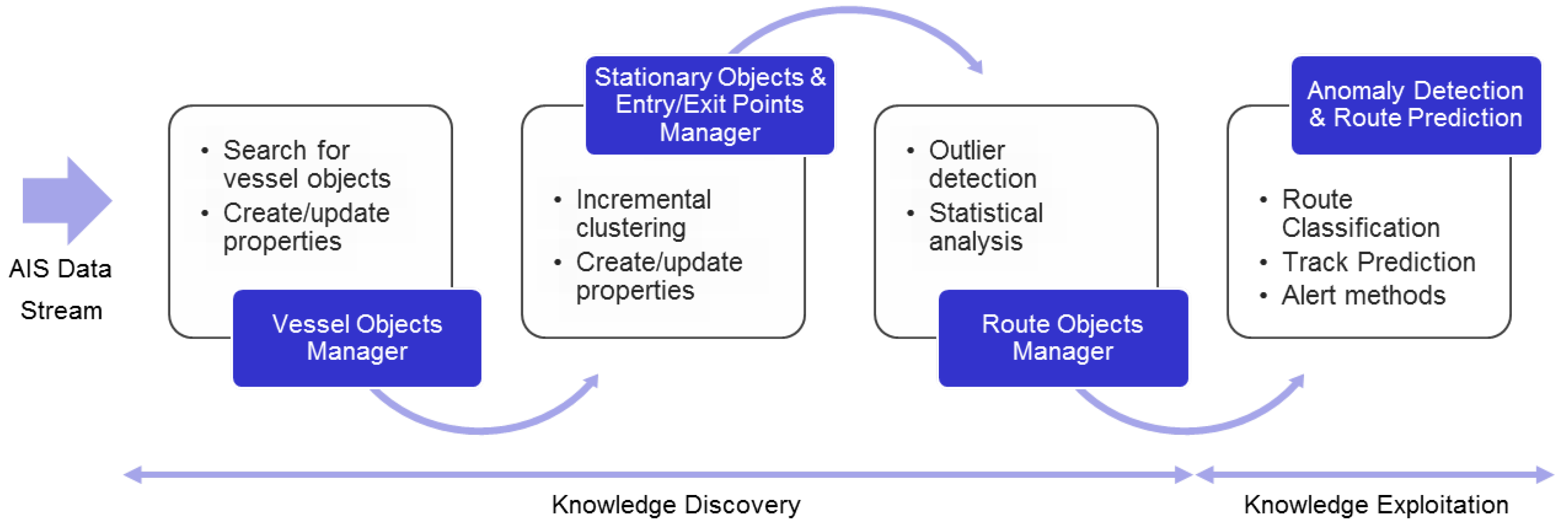
TREAD Functional Architecture Manager: the discovery and exploitation of maritime traffic knowledge-based on AIS information follows the functional architecture shown in Figure 1; the stream of AIS messages is processed to incrementally learn maritime motion patterns through the “Vessel Objects Manager” activated by relevant events based on the temporal and spatial characterization of vessel behavior. The clustering of such events leads to the discovery of waypoints (stationary objects and entry/exit points). The knowledge discovery process is followed by potential exploitation, such as in route classification, prediction and anomaly detection.

Figure 1. Knowledge discovery functional architecture: historical database or real-time data stream of Automatic Identification System (AIS) messages is sequentially processed to incrementally learn maritime motion patterns through processes (“managers”) activated by relevant events. The knowledge discovery process is followed by on-line exploitation, such as route classification, prediction and anomaly detection.

Figure 1. Knowledge discovery functional architecture: historical database or real-time data stream of Automatic Identification System (AIS) messages is sequentially processed to incrementally learn maritime motion patterns through processes (“managers”) activated by relevant events. The knowledge discovery process is followed by on-line exploitation, such as route classification, prediction and anomaly detection.

Vessel Objects Manager: As soon as a new vessel enters the monitored scene, a detection occurs, and the management of vessel objects is initialized (see Algorithm 1-Unsupervised Route Extraction, Annex A). The list of vessel objects, $Vs$, is updated according to the information content of each decoded AIS message (or database record when performing historical data analysis). Every vessel object, $Vs\left\{MMSI\right\}$, is identified by the MMSI number and contains both static and dynamic properties. While the former are linked to the identification of the vessel (e.g., type, call sign, name, International Maritime Organization (IMO) number, size), the latter are related to the state vector (e.g., position, Course Over Ground (COG), Speed Over Ground (SOG)) and to historical and current route patterns). These properties are progressively updated when new data become available. With reference to Algorithm 1—Unsupervised Route Extraction in Annex A—the $Vs\left\{MMSI\right\}.track$ refers to the timestamped history of observed state vector information (i.e., position and velocity parameters) for the vessel object, $Vs\left\{MMSI\right\}$.

Algorithm 1 $UnsupervisedRouteExtraction$

Require: $messages$ // AIS messages containing static and dynamic info, e.g., $MMSI$, $COG$, $SOG$, x, y, $timestamp$

Require: τ // time needed before labeling the vessel as being ‘lost’

Require: $Vs,ENs,POs,EXs,Rs$ // list of vessel, waypoint and route objects

Require: $N_{ENs},N_{POs},N_{EXs},Ep{s}_{ENs},Ep{s}_{POs},Ep{s}_{EXs}$ // clustering parameters (see Algorithm 2)

1: for all $message\in messages$ do 2:   if $not(Vs\{MMSI\})$ then 3:       // the vessel object identified by $MMSI$ does not exist: it is added to the $Vs$ list, its status initialized as ‘sailing’, an entry event generated to be analyzed for $ENs$ objects clustering and the routes list $Rs$ updated 4:       $Vs\leftarrow add(Vs\{MMSI\})$ 5:       $Vs\left\{MMSI\right\}.status\leftarrow ($‘sailing’) 6:       $Vs\left\{MMSI\right\}.track\leftarrow (x,y,COG,SOG,timestamp,\dots )$ 7:       $[Rs,ENs,Vs\left\{MMSI\right\}]\leftarrow Online\_WPs\_Clustering(ENs,Vs\left\{MMSI\right\},Ep{s}_{ENs},N_{ENs})$ // see Algorithm 2 8:       $[Rs,Vs\{MMSI\left\}\right]\leftarrow Route\_Objects\_Manager(Rs,Vs\{MMSI\})$ // (see Algorithm 3) 9:   else 10:       // the vessel exists: its parameters are updated and tested 11:       $Vs\left\{MMSI\right\}.track(end+1)\leftarrow (x,y,COG,SOG,timestamp,\dots )$ 12:       $Vs\left\{MMSI\right\}.avg\_speed={\Delta }_{pos}/{\Delta }_t$   // observed average speed shown by the vessel 13:       if $Vs\left\{MMSI\right\}.avg\_speed<min\_speed$ and $Vs\left\{MMSI\right\}.status=$‘sailing’ then 14:             // the vessel has stopped and a stationary event generated that is considered for POs (ports and offshore platforms) object clustering 15:             $Vs\left\{MMSI\right\}.status\leftarrow ($‘stationary’) 16:             $[Rs,POs,Vs\left\{MMSI\right\}]\leftarrow Online\_WPs\_Clustering(POs,Vs\left\{MMSI\right\},Ep{s}_{POs},N_{POs})$ 17:             $[Rs,Vs\{MMSI\left\}\right]\leftarrow Route\_Objects\_Manager(Rs,Vs\{MMSI\})$ 18:       end if 19:       if $Vs\left\{MMSI\right\}.status=$‘lost’ then 20:             // the vessel is observed again after having been lost (e.g., exited the bounding box area) 21:             $Vs\left\{MMSI\right\}.status\leftarrow ($‘sailing’) 22:             $[Rs,ENs,Vs\left\{MMSI\right\}]\leftarrow Online\_WPs\_Clustering(ENs,Vs\left\{MMSI\right\},Ep{s}_{ENs},N_{ENs})$ 23:             $[Rs,Vs\{MMSI\left\}\right]\leftarrow Route\_Objects\_Manager(Rs,Vs\{MMSI\})$ 24:       end if 25:   end if 26:   // every ${\Delta }_{days}$, look for vessels not having been updated in the last τ time interval and update the $EXs$ list 27:   if mod$(timestamp,{\Delta }_{days})=0$ then 28:       for all $v\in Vs$ do 29:             if $v.last\_update>\tau$ and $v.status\ne ($‘lost’) then 30:                     // the last recorded position of the vessel is used to modify the $EXs$ list, to update the list of vessel waypoints and to create/update the routes, $Rs$ 31:                     $v.status\leftarrow ($‘lost’) 32:                     $[Rs,EXs,v]\leftarrow Online\_WPs\_Clustering(EXs,v,Ep{s}_{EXs},N_{EXs}))$ 33:                     $[Rs,v]\leftarrow Route\_Objects\_Manager(Rs,v)$ 34:             end if 35:       end for 36:   end if 37: end for 38: return $Vs,EXs,ENs,POs,Rs$

From the AIS data stream, the status of vessel objects is derived and updated. Changes of the status of vessel objects are events of interest, such as “lost” when not observed for a time τ, which is a multiple of the maximum AIS message refresh rate in the area of interest. Additional vessel statuses are “stationary”/“sailing”, and their transitions identify other events of interest, such as when the vessel stops or starts sailing again from a stoppage. Such events create or update waypoint objects, $WPs$, as shown in Annex A, Algorithm 1—Unsupervised Route Extraction—and Algorithm 2—On-Line WPs Clustering.

Algorithm 2 $On–lineWPsClustering$

Require:  $Vs,v$ // list of all vessels, $Vs$, and vessel, v, that generated the event of interest to be clustered Require:  $WPs,Rs$ // list of waypoints to be clustered, i.e., either $ENs$, $EXs$ or $POs$, and routes to be modified Require:  $Eps,N$ // minimum number of points, N, in the $Eps$ neighborhood of the event located in $v.track(end)$ that is required to generate a cluster $w{p}_n\in WPs$

1: $[WPs,op]\leftarrow Incremental\_DBSCAN(WPs,v.track(end),N,Eps)$ // see Incremental DBSCAN in [37]. 2: if $op=$‘none’ then 3:   // the event is not clustered and is considered as noise 4:   $v.wps(end+1)\leftarrow ($‘Unclassified Waypoint’$,v.track(end))$ 5: else 6:   // the operation performed in the WPs space is either the generation of a new waypoint, the absorption into an existing one or the merge of multiple waypoints: 7:   if $op=$‘new cluster’ then 8:       //the event has created a new cluster, $w{p}_n$, the vessel list of waypoints is updated together with the time, $timestam{p}_{w{p}_n}$, of information, as extracted from $v.track(end)$ 9:       $WPs\leftarrow add($‘WP${}_n$’) 10:       $v.wps(end+1)\leftarrow ($‘WP${}_n$’) 11:       $v.timestam{p}_{wp}(end+1)\leftarrow (v.track(end))$ 12:       // info regarding the $MMSI$ of the vessel and its last position is recorded into $w{p}_n$ 13:       $[w{p}_n.List\_MMSIs(end+1),w{p}_n.tracks(end+1)]\leftarrow (v.MMSI,v.track(end))$ 14:   end if 15:   if $op=$‘cluster expanded’ then 16:       // the event is absorbed into the cluster, $w{p}_n$: 17:       $v.wps(end+1)\leftarrow ($‘WP${}_n$’) 18:       $v.timestam{p}_{wp}(end+1)\leftarrow (v.track(end))$ 19:       $[w{p}_n.List\_MMSIs(end+1),w{p}_n.tracks(end+1)]\leftarrow (v.MMSI,v.track(end))$ 20:   end if 21:   if $op=$‘clusters merged’ then 22:       // the new event causes the merging of two clusters, $w{p}_m$ and $w{p}_n$, into $w{p}_n$, the event is clustered, $w{p}_n$ updated and, finally, $w{p}_m$ deleted. 23:       $v.wps(end+1)\leftarrow ($‘WP${}_n$’) 24:       $v.timestam{p}_{wp}(end+1)\leftarrow (v.track(end))$ 25:       $w{p}_n\leftarrow (v.MMSI,v.track(end))$ 26:       $w{p}_n\leftarrow merge(w{p}_n,w{p}_m)$ 27:       for all $\widehat{v}\in Vs\{MMSI=w{p}_m.List\_MMSIs\}$ do 28:             $\widehat{v}.wps(\widehat{v}.wps=$‘WP${}_m$’$)\leftarrow ($‘WP${}_n$’) 29:       end for 30:       // merge the affected routes and update the relevant list 31:       for all $\widehat{R}\in (R_s.wps(1)=$‘WP${}_m$’$|R_s.wps(2)=$‘WP${}_m$’) do 32:             $\tilde{R}\leftarrow (R_s.wps(\widehat{R}.wps=$ ‘WP${}_m$’) = ‘WP${}_n$’) 33:             $\tilde{R}\leftarrow merge(\tilde{R},\widehat{R})$ 34:             $delete(\widehat{R})$ 35:       end for 36:       $delete($‘WP${}_m$’) 37:   end if 38: end if 39: return $WPs,v,Rs$

Stationary Objects Manager: A special class of waypoints is represented by stationary points, such as ports and offshore platforms, $POs$. This class of objects consists of vessels having a speed lower than a given threshold. In particular, as can be seen in Annex A, Algorithm 1—Unsupervised Route Extraction—stationary events are detected by speed gating based on the last observations related to the vessel of interest: the parameters, ${\Delta }_t$ and ${\Delta }_{pos}$ (i.e., the last observed time interval and the resulting displacement in position), are computed to empirically derive the average vessel speed. This is implemented, since the field, $SOG$, in the AIS messages is unreliable to be used in detecting stationary events. Port and offshore platforms are learned by clustering the stationary behavior of vessels, and their areas are progressively shaped by vessels following the same behavior. Waypoints clustering is based on DBSCAN (i.e., Density-Based Spatial Clustering of Applications with Noise) methodology ([38]). DBSCAN forms clusters of elements on the basis of the density of points in their neighborhood. In other words, given a specific point, p, if the cardinality of the neighborhood of a given radius, Eps, is greater than a certain threshold of the minimum number of points, then such points are density-reachable from p and belong to the same cluster. Moreover, two points, p and q, are density-connected if there is a third point, o, such that p and q are density-reachable from o. Points that are density-connected to each other belong to the same cluster, and points that are density-connected to any point of the cluster are also part of the cluster. In this framework, those points that are not density-connected to other points do not belong to any cluster and are considered noise.

Algorithm 3 $RouteObjectsManager$

Require: v, $WPs (i.e., ENs,EXs,POs)$, $Rs$

1: // if the vessel has passed through at least two waypoints  2: if $length(v.wps)>1$ then  3:   $[w{p}_a,w{p}_b]\leftarrow v.wps(end-1:end)$  4:   if $not(Rs\{w{p}_a\_to\_w{p}_b\})$ then  5:       //the route from $w{p}_a$ to $w{p}_b$ does not exist: it is added to the $Rs$ list  6:       $Rs\leftarrow add(Rs\{w{p}_a\_to\_w{p}_b\})$  7:   end if  8:   // update the relevant route by adding the track portion between $w{p}_a$ and $w{p}_b$  9:   $timestam{p}_{w{p}_a}=v.timestam{p}_{wp}(v.wps=w{p}_a)$ 10:   $timestam{p}_{w{p}_b}=v.timestam{p}_{wp}(v.wps=w{p}_b)$ 11:   $Rs\{w{p}_a\_to\_w{p}_b\}.params(end+1)\leftarrow (v.track(timestamp\in [timestam{p}_{w{p}_a},timestam{p}_{w{p}_b}]))$ 12:   // update the vessel list of routes 13:   $v.routes\leftarrow add($‘$Rs\{w{p}_a\_to\_w{p}_b\}$’) 14: end if 15: return $v,Rs$

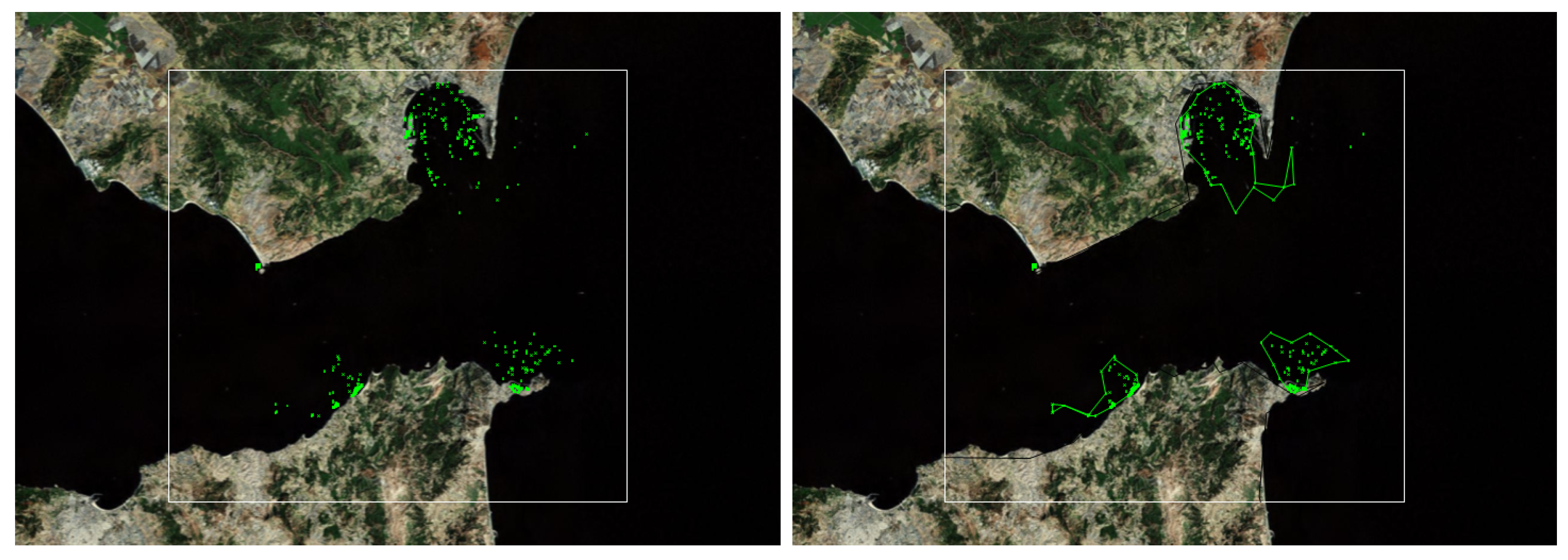
Differently from centroid-based clustering, DBSCAN does not require the number of clusters a priori, while arbitrarily shaped clusters can be easily found as often observed within the maritime traffic context. For instance, centroid-based methods can fail in discriminating different ports whose centroids are close to each other, when they are located along the coast line, as shown in Figure 2. Moreover, DBSCAN introduces a way to classify noise points, which can be used to detect and filter outliers, as will be shown hereafter.

The on-line learning enables an incremental density-based clustering of waypoints. The waypoints clusters are either created, expanded and merged, following the typical procedure of incremental DBSCAN, as introduced in [37]. In Algorithm 2, the on-line clustering of $WPs$ is illustrated, showing how the vessel object features are updated accordingly. The cluster parameters (i.e., the radius, $Eps$, of the neighborhood of the event of interest and the minimum number, N, of points to be detected in the $Eps$-neighborhood of the vessel) are tuned, based on the specific nature of the $WPs$ (i.e., whether they are $POs$ or $ENs$/$EXs$ objects) and on the specific features of the monitored area.

Topographically, port and offshore platform objects are represented via a spatial distribution given by the coordinates of the vessels, which contribute to create or update them. As a consequence, such objects are automatically described via a list of vessel objects and a volume of traffic. In this way, a frequency plot based on the type of vessels can be associated to each port and offshore platform object in order to help characterize the activities in the stop zones.

Figure 2. Stationary points (green dots) incrementally detected during a two-week period over the Strait of Gibraltar, an area characterized by intense traffic. Stationary points are then clustered using incremental Density-Based Spatial Clustering of Applications with Noise (DBSCAN) into port and offshore platform objects, whose concave hulls (right) consistently capture areas where vessels anchor outside ports.

Figure 2. Stationary points (green dots) incrementally detected during a two-week period over the Strait of Gibraltar, an area characterized by intense traffic. Stationary points are then clustered using incremental Density-Based Spatial Clustering of Applications with Noise (DBSCAN) into port and offshore platform objects, whose concave hulls (right) consistently capture areas where vessels anchor outside ports.

Entry and Exit Points Manager: Another class of waypoints useful for describing the motion patterns within a selected area is represented by entry ($ENs$) and exit ($EXs$) points. Whenever a vessel object enters (leaves) the area under analysis, it generates “birth”/“death” events (corresponding to vessel status transition “transmitting”/“lost” and vice versa), and the relevant entry/exit point is created or updated. As in image processing and visual surveillance (see, e.g., [16]), entry and exit points are related to the monitored scene and may change depending on the bounding box area, while port or offshore platform objects are fixed reference points. Similarly to the stationary points, entry and exit points are learned through the incremental DBSCAN method and described with a list of transiting vessel objects and a volume of traffic. Algorithm 2—On-Line WPs Clustering in Annex A summarizes the main steps. 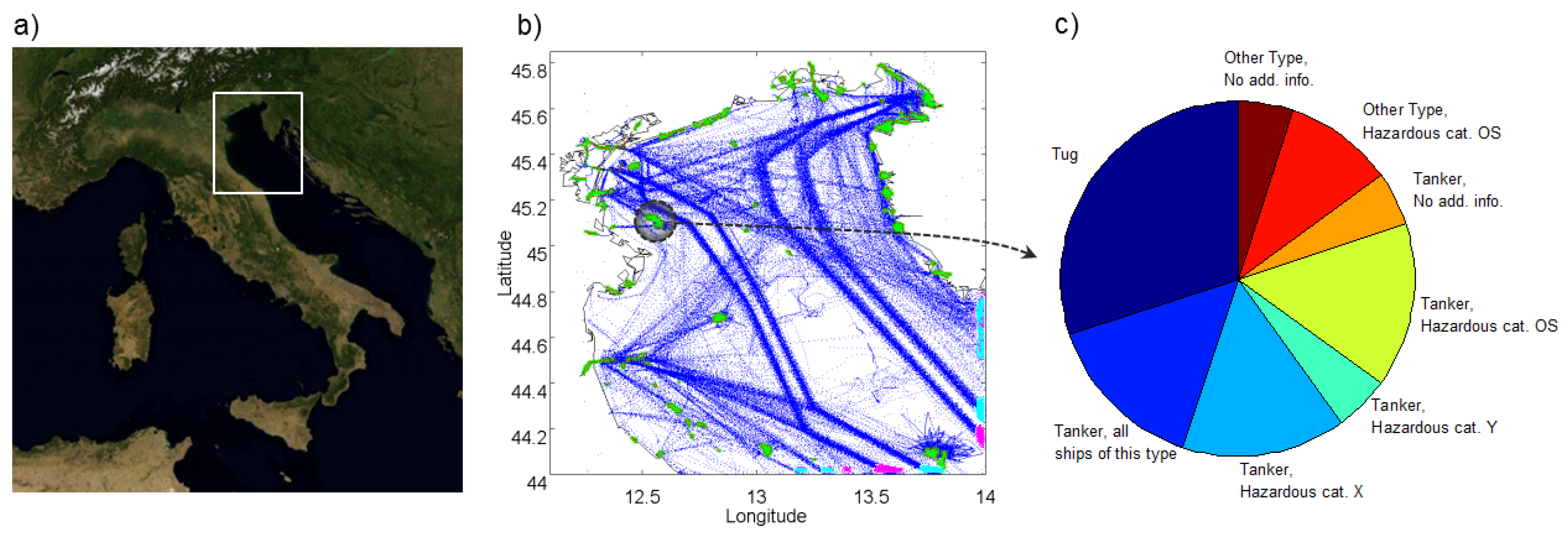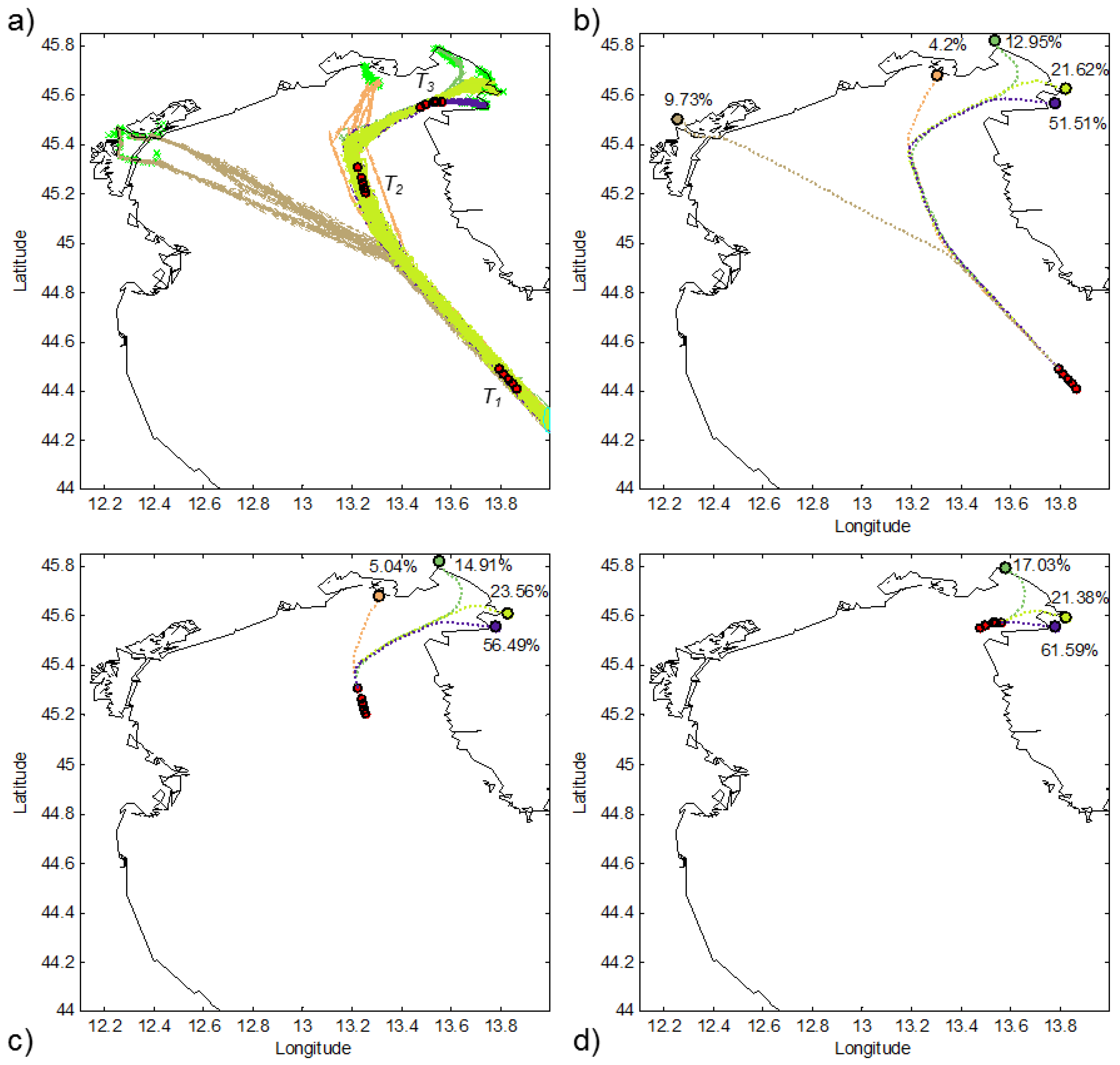Figure 3 shows the results of the unsupervised waypoints detection and characterization over the North Adriatic Sea, where many routing systems are present (such as traffic separation schemes), because of the intense traffic and oil drilling activities.

Route Objects Manager: Once the waypoints are learned, route objects, $Rs$, can be built by clustering the extracted vessel flows, which connect two ports (i.e., local routes), an entry point to a port, a port and an exit point or an entry point and an exit point (i.e., transit routes). Route objects do not merely count the registered transiting vessels, but are also statistically described by the static and kinematic features of the vessels that created or updated them.

Specifically, the Route Objects Manager, whose main steps are reported in Algorithm 3—Route Objects Manager in Annex A—deals with the creation of new route objects and with the dynamic management of their features and labels, as resulting from the incremental clustering of the relevant $WPs$ described in Algorithm 2—On-Line WPs Clustering, Annex A.

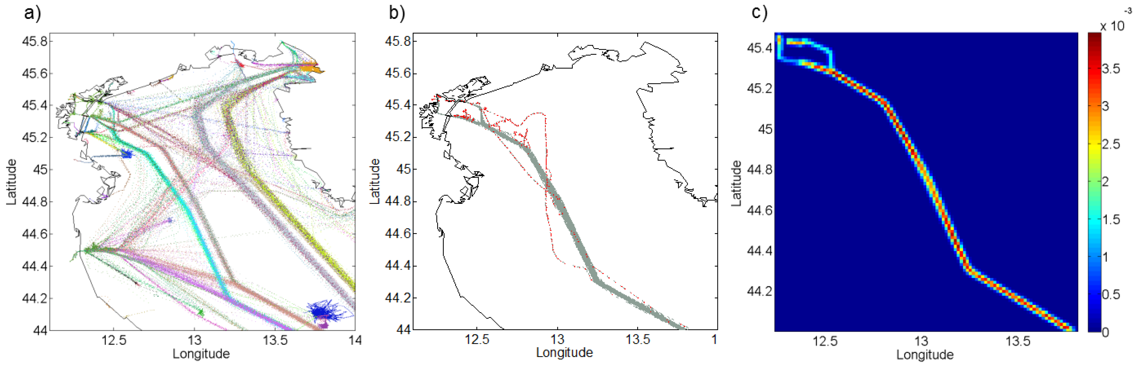
Figure 3. Waypoints detection and characterization over a $200\times 160$ km area in the North Adriatic Sea (a) from March 1 to May 15, 2012. The unsupervised analysis leads to the detection of entry (cyan), exit (magenta) and stationary areas (green) (b), one of them being an offshore regasification gateway as confirmed by the ship type distribution analysis (c), following the categorization in [39], performed on the Maritime Mobile Service Identity (MMSI) list of registered vessels.

Figure 3. Waypoints detection and characterization over a $200\times 160$ km area in the North Adriatic Sea (a) from March 1 to May 15, 2012. The unsupervised analysis leads to the detection of entry (cyan), exit (magenta) and stationary areas (green) (b), one of them being an offshore regasification gateway as confirmed by the ship type distribution analysis (c), following the categorization in [39], performed on the Maritime Mobile Service Identity (MMSI) list of registered vessels.

Once a vessel enters the scene, its features are compared with the existing set of routes. If a route already exists, whose positional features are compatible to the vessel features, both the vessel is added to the route list of vessels and, mutually, the route is added to the list of the $WPs$ transited by the vessel. 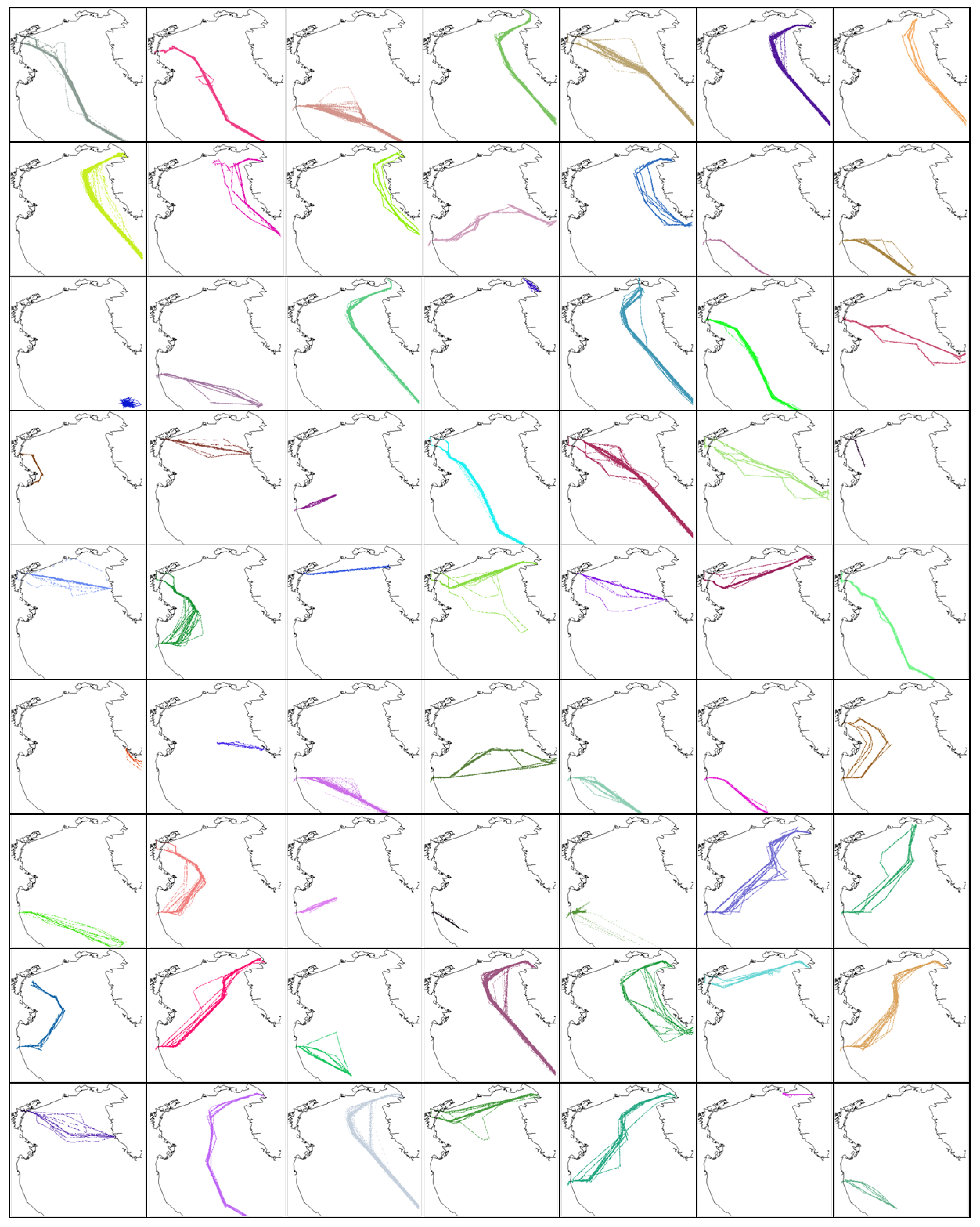Otherwise, the vessel contributes to the initialization of a new route, and, when a minimum number of detections (i.e., number of transits along the route) is reached, the new route is activated. Each route object has a spatio-temporal sequence of state vectors, facilitating the analysis and classification of activities. The detected routes can be organized in historical atlases, which summarize the maritime traffic in the considered area. As an example, we report the route codebook learned in the North Adriatic Sea in Figure 4. Some of the derived routes are not easy to explain by glancing at the AIS traffic messages reported in Figure 3b. The methodology shows a significant agreement with the traffic schemes in use on nautical charts.

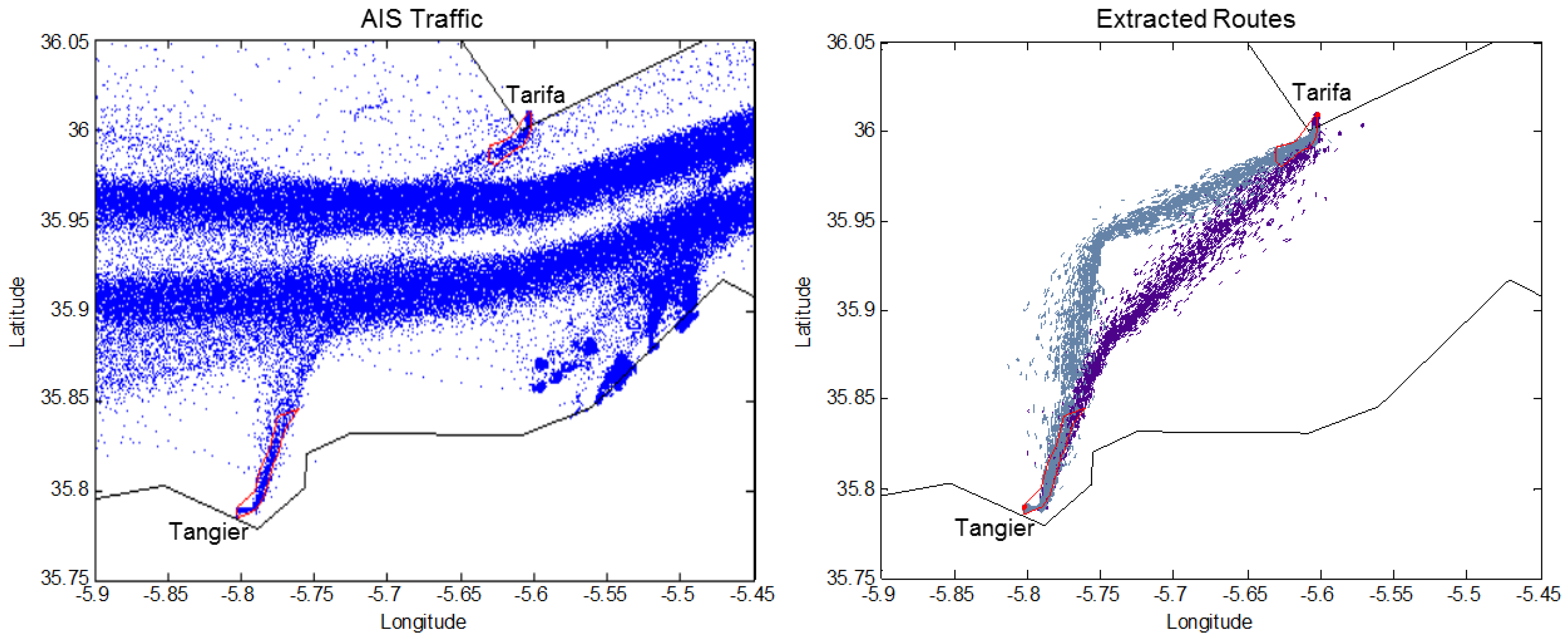
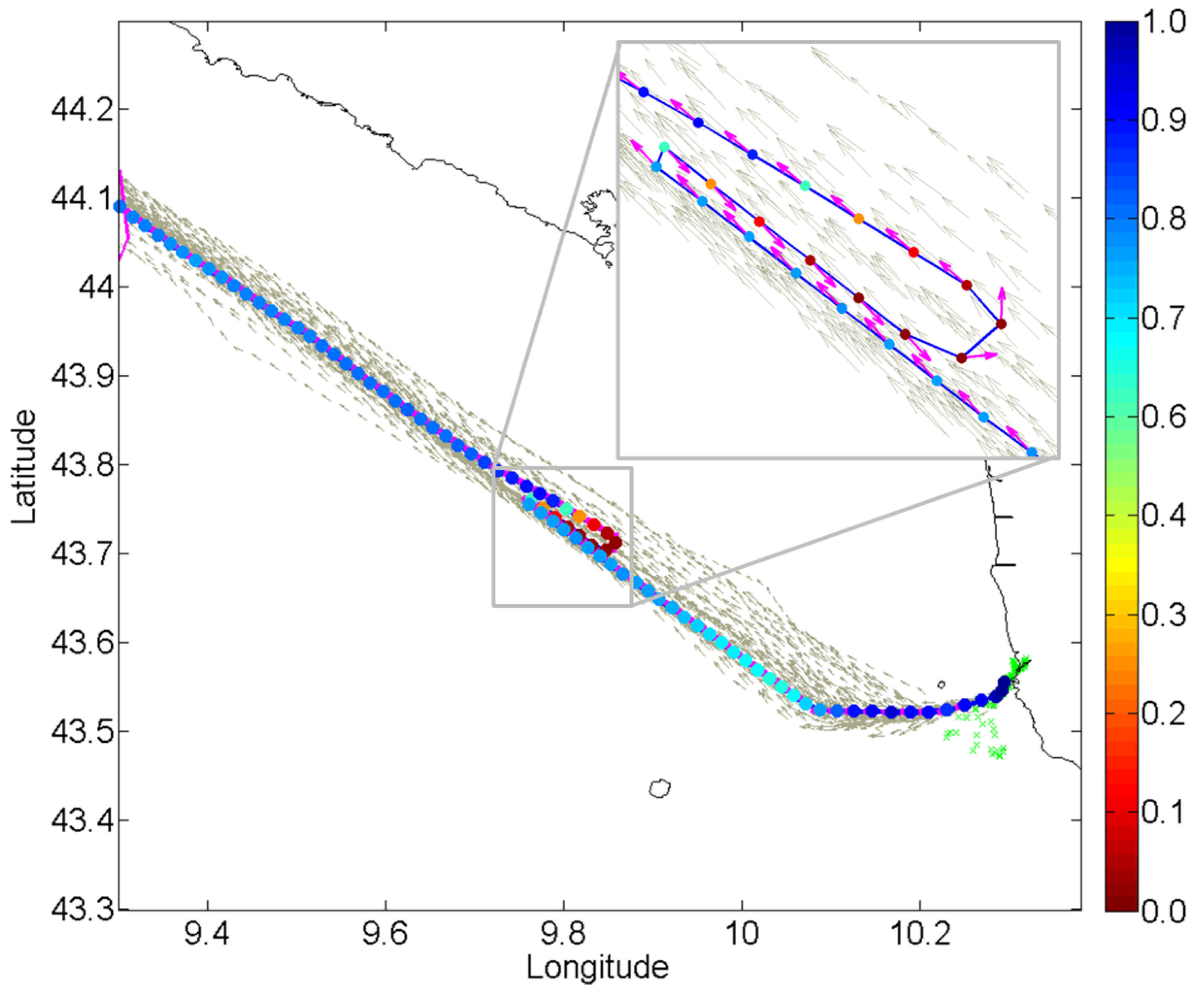
In Figure 5, an example of two routes extracted between two detected stationary areas in the Strait of Gibraltar is illustrated. The major east and westbound traffic volumes significantly exceed the traffic flow between the selected ports, making the routes’ visual isolation difficult.

The two routes adhere to the maritime rules of the road when crossing the main traffic flows: the main traffic in the same direction flow is crossed at a shallow angle (i.e., ${20}^{\circ }$–${30}^{\circ }$), while the opposing traffic flow in each route is cut across at broad angles (i.e., ${90}^{\circ }$). The second portion of each route is, therefore, more diffuse, as the ferries maneuver more when crossing the opposing sea lanes compared to overtaking traffic in the same direction. 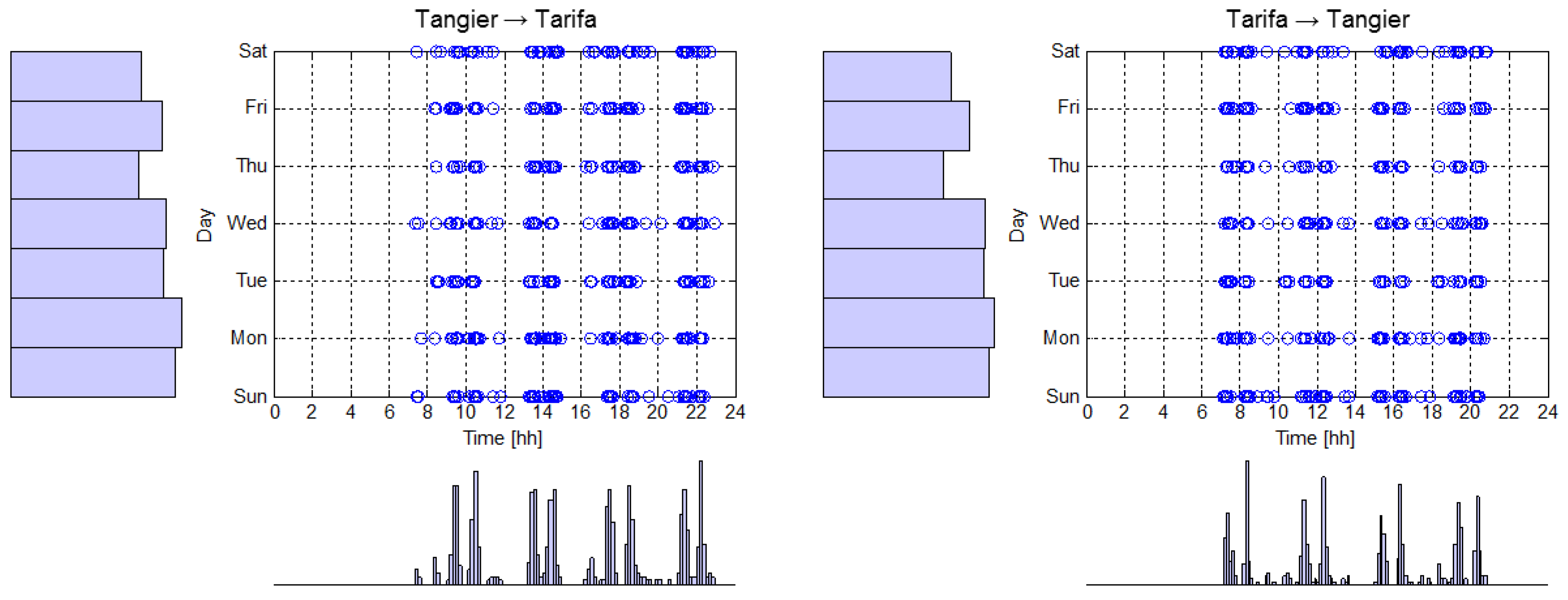The extracted routes, whose number is not assumed a priori, but automatically learned, are characterized also by the information of the entering and exiting time of the registered vessels together with their ship type. Different from live video analysis applications, this allows the extraction of higher level information, such as the ship type, distribution of the route, its average travel time and the daily/weekly patterns, as shown in Figure 6.

Figure 4. Set of highly dense routes into which the traffic in Figure 3 was decomposed.

Figure 4. Set of highly dense routes into which the traffic in Figure 3 was decomposed.

Anomalies in the traffic schedule can therefore be modeled on vessels that are fully compliant with the route directions, but use them at low-likelihood times. Detected route objects often show trajectories that share the same entering and exiting waypoints, but their path considerably deviates from other vessel paths within the same route. It is necessary to discard those outliers, so that anomaly detection can be performed based on a more representative picture of the vessel normal traffic, as is commonly done in statistical process control and change detection practice. Thus, anomaly detection is related to, but differs from, noise removal in the data: noise works as an obstruction to data analysis and is not of primary interest to the analyst. Undesired outliers must be removed before further knowledge exploitation can be performed. This pre-processing phase is implemented by using the DBSCAN method. Specifically, it includes the classification of route points as core points, border points and noise points. Noise points are not considered representative of historical patterns and are filtered out. An example of a pre-processed route is reported in Figure 7b. As highlighted in [8], vessels typically follow traffic sea lanes that are sequences of straight lines. The Gaussian Mixture Models (GMM), very popular in the pattern recognition literature, can be used to fit the distribution of position data points. Along the minor axis perpendicular to the lane, the Gaussian models can capture the vessel position variability and displacements. However, along the major axis, the vessel distribution is assumed to be approximately uniform, and thus, the Gaussian distribution is a sub-optimal spatial density model. So, a non-parametric approach can be more appropriate to model the two-dimensional traffic density distribution and has been adopted in the present work. Among the non-parametric approaches, Kernel Density Estimation (KDE) is a common technique for estimating the unknown probability density function (pdf) of the random variable “vessel position”. Compared to GMM, KDE makes no assumption about the parametric model of the underlying pdf, whose form is estimated using historical data samples. Moreover, KDE does not need to specify the number of components of the mixture model, which is one of the main drawbacks of GMM. For these reasons, KDE has shown a superior ability to accurately model traffic lanes. Figure 7c reports the KDE representation of a refined route, adopting a Gaussian kernel with an optimized bandwidth selection based on the Minimization of a Cost function.

Figure 5. AIS traffic data in proximity of the Strait of Gibraltar (left) collected over two months, and (right) extracted routes between the learned port of Tarifa and the old port of Tangier, both highlighted in red.

Figure 5. AIS traffic data in proximity of the Strait of Gibraltar (left) collected over two months, and (right) extracted routes between the learned port of Tarifa and the old port of Tangier, both highlighted in red.

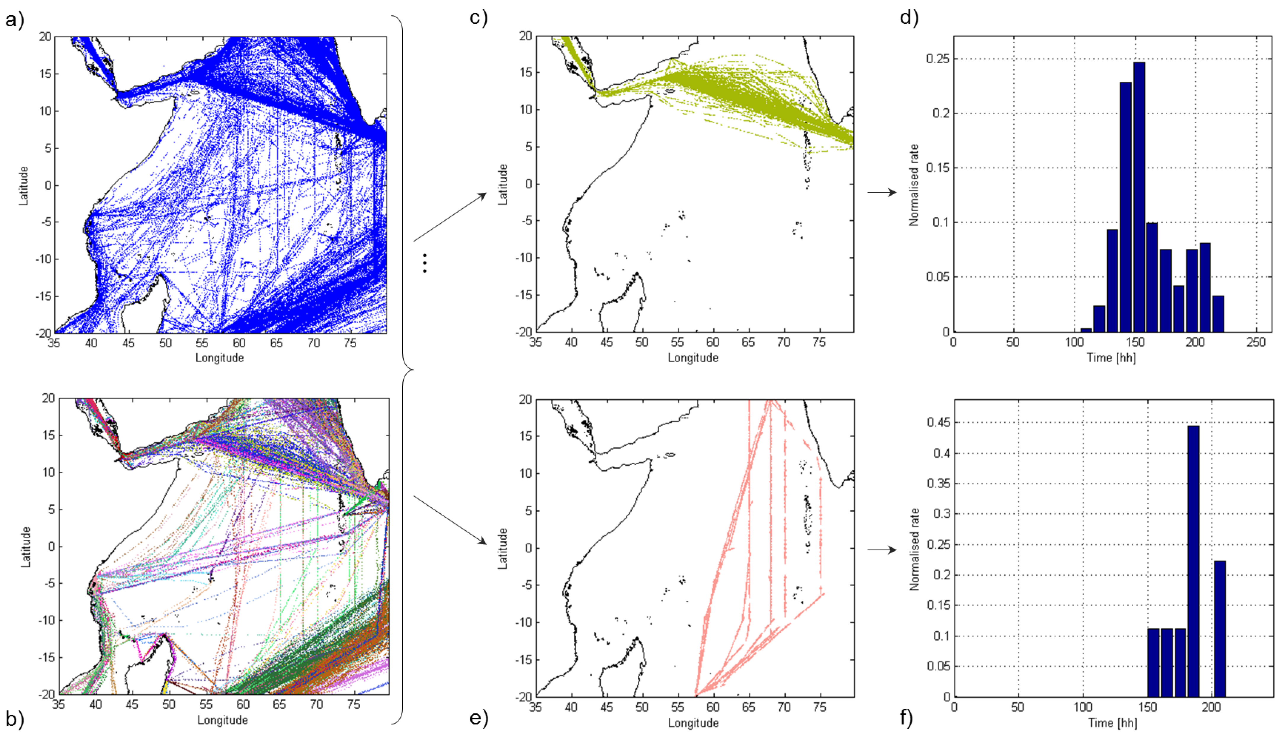
TREAD was tested in different areas and using data from different AIS sources (i.e., terrestrial and satellite AIS). Figure 8 shows an example of the traffic knowledge learned using satellite AIS data in the Indian Ocean. It is noteworthy that some of the routes displayed in Figure 8b are not easily anticipated by simply looking at the raw AIS traffic data in Figure 8a. As an example, the route from the Suez Canal to the Laccadive Sea (Figure 8c) is firstly constrained by the Internationally Recommended Transit Corridor (IRTC) and easily isolated. Then, it becomes more disperse outside the routing system and more difficult to be identified. The spatial spread of the second route in Figure 8e shows how the effects of piracy have modified the common routes over the Indian Ocean near Somalia, due to high-risk areas.

Figure 6. Daily patterns between northbound (left) and southbound (right) routes covered by four ferries whose schedule can be derived by the multiple peaks of the time histograms on the bottom.

Figure 6. Daily patterns between northbound (left) and southbound (right) routes covered by four ferries whose schedule can be derived by the multiple peaks of the time histograms on the bottom.

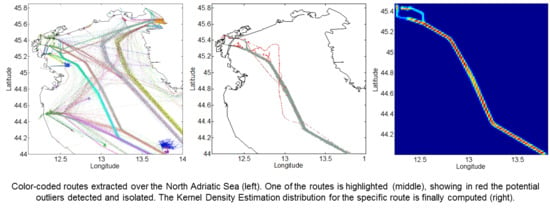
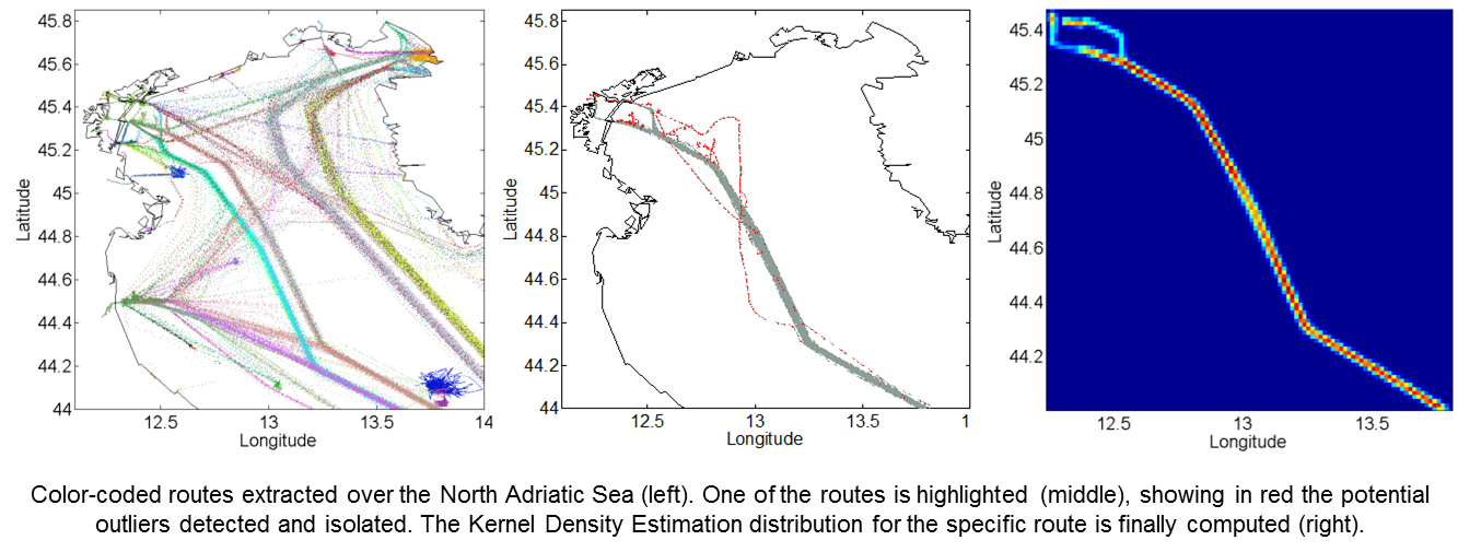
Figure 7. Color-coded routes (a) extracted over the area in Figure 3, showing patterns not clearly visible by analyzing traffic density data (see Figure 3b); one of them (b) is highlighted, showing in red the potential outliers detected and isolated using density-based clustering on the route points. The Kernel Density Estimation (KDE) distribution for the specific route is finally computed (c).

Figure 7. Color-coded routes (a) extracted over the area in Figure 3, showing patterns not clearly visible by analyzing traffic density data (see Figure 3b); one of them (b) is highlighted, showing in red the potential outliers detected and isolated using density-based clustering on the route points. The Kernel Density Estimation (KDE) distribution for the specific route is finally computed (c).

At last, each route can be decomposed into the elementary trajectories followed by all the vessels belonging to that route, thus facilitating the search for tracks that deviate from “normality”. When a vessel object is instantiated, its features are compared with all the routes already present in the database performing Route Classification (see Section 4.1).

Figure 8. Three-month satellite AIS positioning data over the Indian Ocean (a); superposition of detected routes (b). Two of them are further analyzed in terms of spatial (c and e) and travel times distribution (d and f).

Figure 8. Three-month satellite AIS positioning data over the Indian Ocean (a); superposition of detected routes (b). Two of them are further analyzed in terms of spatial (c and e) and travel times distribution (d and f).

3.1. Learning Performance and Traffic Entropy

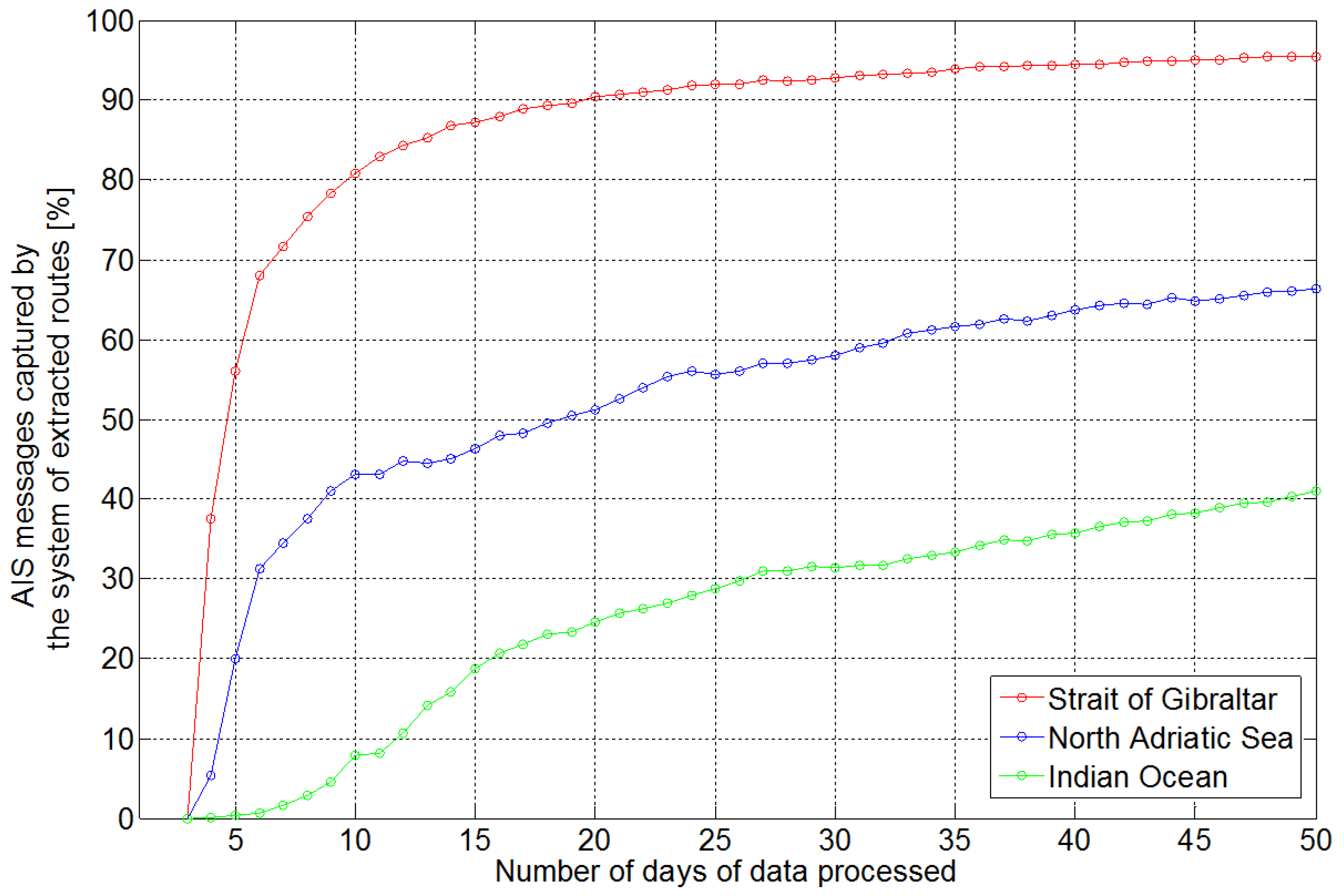
The learning performance of TREAD methodology was analyzed in terms of the ratio between the number of AIS messages mapped into the extracted system of routes and the number of processed positioning messages. Figure 9 shows the learning results on 50-day ground based data over the Strait of Gibraltar and the North Adriatic Sea and satellite-based data over the Indian Ocean as introduced by Figure 3b, Figure 5a and Figure 8, respectively. After a common preliminary phase when the system constructs the entry/exit and stationary point objects, the learning accuracy performance stabilizes at different levels, depending on traffic density and constraints. Thus, the more the traffic is constrained or regulated, the more accurate the unsupervised learning results. The extremely high traffic density and rigid routing system allowed the Strait of Gibraltar to be learned relatively quickly and consistently, capturing up to 95% of the processed messages. Lower accuracy performance can be seen in the North Adriatic Sea, where, despite the relatively constrained traffic, there are opportunities for many routes to be followed within the time window. As a result, only 70% of the traffic is learned. This aspect is even more pronounced in the Indian Ocean, where merely 40% of the traffic can be clustered, due to a lack of traffic constraints over a large area combined with the low update rates of satellite-based AIS data.

The curves in Figure 9 represent the portion of the information that contributes to the historical traffic pattern model versus the amount of processed information. The amount of information that does not contribute to the traffic knowledge discovery is discarded. There is a certain point of diminishing returns, or an upper threshold, for the number of data points, which are included into the learned system of routes, beyond which the additional data do not provide further useful information to the historical route system. The traffic pattern knowledge discovery process can therefore be linked to the notion of entropy, which measures the degree of disorder in a system. Information Theory entropy is widely employed to predict human mobility, Asynchronous Transfer Mode (ATM) traffic streams and cellular network traffic [40]. Entropy clearly provides a measure of the extent to which the traffic can be predicted on the basis of the historical patterns over the area. Within this framework, entropy can be used to quantify the information gain that the derived traffic patterns will provide for prediction [41]. In geographical clustering studies, the notion of entropy has been suggested in [42] and recently applied to detect abnormal activities in video surveillance in [43]. As a consequence, the detection of potential anomalies can be linked to the traffic entropy: the capability to successfully recognize low-likelihood behaviors is enhanced in areas where the traffic patterns are highly regular and, therefore, the associated level of disorder is low.

Figure 9. Portion of AIS messages captured by the learned system of routes over the reported areas of interest.

Figure 9. Portion of AIS messages captured by the learned system of routes over the reported areas of interest.

Thus, while the learning rate depends on the traffic density, the end state knowledge discovery performance is affected by the different levels of traffic entropy over the area of interest and will vary from region to region.

4. Routes Knowledge Exploitation

Similarly to [12,15], once the picture of the maritime traffic is constructed, the historical knowledge can be used to (i) classify the routes, assigning to each of them a probability that the vessel is actually following it, (ii) predict the future route along which a vessel is going to move, in agreement with the partially observed track and given the vessel static information and (iii) detect anomalous behaviors that deviate from the learned traffic normality.

4.1. Route Classification

Classifying a set of vessel positioning observations into specific routes is crucial for augmenting the situational awareness over the maritime traffic area. Route classification assigns a probability to each route compatible to the vessel position. This is expressed as the posterior probability that the vessel belongs to that specific route, having observed a partial vessel track. Generally speaking, a vessel track, $\mathbf{V}$, is a time series of T observed state vectors, ${\mathbf{v}}_i$:

$$\mathbf{V}=\{{\mathbf{v}}_1,{\mathbf{v}}_2,\dots ,{\mathbf{v}}_T\}$$

(1)

where the state vector observation, ${\mathbf{v}}_t$, is directly isolated from the broadcast AIS information. In this study, it includes both position and velocity information as extracted by the vessel track properties, $v.track$ (see Section 3):

$${\mathbf{v}}_t={[x_t,y_t,{\dot{x}}_t,{\dot{y}}_t]}^{⊺}$$

(2)

where $x_t$ and $y_t$ are related to the vessel coordinates and the velocity components, ${\dot{x}}_t$ and ${\dot{y}}_t$, are derived by combining SOG and COGinformation, based on the conditions: ${\text{SOG}}_t=\sqrt{{\dot{x}}_t^2+{\dot{y}}_t^2}$ and ${\text{COG}}_t=ta{n}^{-1}\left(\frac{{\dot{y}}_t}{{\dot{x}}_t}\right)$

The vessel track, $\mathbf{V}$, can be associated to a time series of regions, $\overline{\mathbf{S}}=\{{\mathbf{s}}_1,{\mathbf{s}}_2,\dots ,{\mathbf{s}}_T\}$, spatially identified by circles of radius d centered in the observed positions, $[x_t,y_t]$, which represent the temporal sequence of states and take into account the time lags, ${\Delta }_t$, between subsequent observations. The spatial region identified by the $t-th$ state, ${\mathbf{s}}_t$, as further discussed hereafter, can be used as a mask to capture the route elements in the neighborhood of the observation, ${\mathbf{v}}_t$, subsequently used to characterize the local route behavior. It is clear that the selection of the distance, d, and, therefore, the size of the state regions, affect the route classification effectiveness: if d is too small, the characterization of the local route behavior would be based on a reduced number of neighbors, leading to poor generalization capabilities. Similarly, if d is too large, the characterization would be biased by the mixing of different behaviors (e.g., as in the case of non-rectilinear routes). This is illustrated by Figure 10.

It has been found that state regions with a radius d in the order of a few nautical miles lead to acceptable classification results independently of the route spatial and directional dispersion.

Each AIS message can be decoded to derive the vessel type, c, according to the categorization in [39]. The classification problem lies in finding the route, $R_c^{k^{*}}$, that maximizes the posterior probability, $P(R_c^k|\mathbf{V},\overline{\mathbf{S}})$, over the $k=1,...,K$ possible compatible routes $R_c^k\in Rs$ (see Section 3):

$$R_c^{k^{*}}=\underset{k}{argmax}P(R_c^k|\mathbf{V},\overline{\mathbf{S}})$$

(3)

where, following the Bayes rule, $P(R_c^k|\mathbf{V},\overline{\mathbf{S}})$, can be decomposed as follows:

$$P(R_c^k|\mathbf{V},\overline{\mathbf{S}})\propto P(\mathbf{V},\overline{\mathbf{S}}|R_c^k)P(R_c^k)$$

(4)

Figure 10. Example of observed vessel track, $\{{\mathbf{v}}_{t-2},{\mathbf{v}}_{t-1},{\mathbf{v}}_t\}$ (red), associated temporal state sequence, $\{{\mathbf{s}}_{t-2},{\mathbf{s}}_{t-1},{\mathbf{s}}_t\}$ (circles) and points (blue) of a compatible route, as resulting from the traffic knowledge discovery process. If the selected radius is too large (e.g., $d^{\prime }>d$), distinct local directional distributions can be included into the same state, biasing the motion characterization of the relevant observation neighborhood and, thus, the route classification process.

Figure 10. Example of observed vessel track, $\{{\mathbf{v}}_{t-2},{\mathbf{v}}_{t-1},{\mathbf{v}}_t\}$ (red), associated temporal state sequence, $\{{\mathbf{s}}_{t-2},{\mathbf{s}}_{t-1},{\mathbf{s}}_t\}$ (circles) and points (blue) of a compatible route, as resulting from the traffic knowledge discovery process. If the selected radius is too large (e.g., $d^{\prime }>d$), distinct local directional distributions can be included into the same state, biasing the motion characterization of the relevant observation neighborhood and, thus, the route classification process.

The prior $P(R_c^k)$ can be empirically evaluated as the ratio of the number of vessels that transited along the route, $R_c^k$, over the total number of vessels detected in the area of interest. The likelihood, $P(\mathbf{V},\overline{\mathbf{S}}|R_c^k)$, accounts for the joint probability of the time series, $\mathbf{V}$, of the observations and the sequence of the states, $\overline{\mathbf{S}}$, compared to the route, $R_c^k$.

Similarly to the probabilistic approach in the Hidden Markov Model (HMM) literature [44] and in the spatio-temporal trajectory mining literature (see, e.g., [45,46]), the joint probability, $P(\mathbf{V},\overline{\mathbf{S}}|R_c^k)$, of the vessel track, $\mathbf{V}$, and states sequence, $\overline{\mathbf{S}}$, given the route, $R_c^k$, can be written as follows:

$$P(\mathbf{V},\overline{\mathbf{S}}|R_c^k)=P(\mathbf{V}|\overline{\mathbf{S}},R_c^k)P(\overline{\mathbf{S}}|R_c^k)$$

(5)

the sequence of states, $\overline{\mathbf{S}}$, being fixed, once the track sequence, $\mathbf{V}$, has been observed. Similar interesting examples can be found in signal processing [47], video tracking [15] and maritime surveillance applications [48].

The probability, $P(\mathbf{V}|\overline{\mathbf{S}},R_c^k)$, of the observation sequence, $\mathbf{V}$, for the state sequence, $\overline{\mathbf{S}}$, given the route, $R_c^k$, can be expressed as follows:

$$P(\mathbf{V}|\overline{\mathbf{S}},R_c^k)=\prod _{t=1}^{T}P({\mathbf{v}}_t|{\mathbf{s}}_t,R_c^k)$$

(6)

In Equation (6), the probability of observing a feature vector, ${\mathbf{v}}_t$, in one state, ${\mathbf{s}}_t$, is assumed to be independent of the feature vectors in other states. This is an approximation, since the feature vectors of the track, $\mathbf{V}$, are related to the same vessel and, hence, are interdependent. Nevertheless, this approximation has been adopted elsewhere (see, e.g., [47]) with satisfying results. The generic $P({\mathbf{v}}_t|{\mathbf{s}}_t,R_c^k)$ is the probability of observing the feature vector, ${\mathbf{v}}_t$, given the elements, $\{R_c^k(\ell ).[x,y,\dot{x},\dot{y}]\}$, of the route, $R_c^k$, within the state region, ${\mathbf{s}}_t$, defined as follows:

$$\{R_c^k(\ell ).[x,y,\dot{x},\dot{y}]\}\text{where}\parallel R_c^k(l).[x,y]-[x_t,y_t]\parallel \le d,\forall l\in \ell$$

(7)

The probability, $P({\mathbf{v}}_t|{\mathbf{s}}_t,R_c^k)$, is calculated as:

$$P({\mathbf{v}}_t|{\mathbf{s}}_t,R_c^k)=P(x_t,y_t,{\dot{x}}_t,{\dot{y}}_t|{\mathbf{s}}_t,R_c^k)=P({\dot{x}}_t,{\dot{y}}_t|x_t,y_t,{\mathbf{s}}_t,R_c^k)P(x_t,y_t|{\mathbf{s}}_t,R_c^k)$$

(8)

where $P({\dot{x}}_t,{\dot{y}}_t|x_t,y_t,{\mathbf{s}}_t,R_c^k)$ is the probability of observing the velocity components, ${\dot{x}}_t$ and ${\dot{y}}_t$, within the state, ${\mathbf{s}}_t$, as identified by the neighbors of the current position, $[x_t,y_t]$, within a distance, d. This conditional probability takes into account the velocity dependency on the area where the vessel is actually observed. In other words, this component tells us the extent to which the vessel velocity vector is in line with the historical speed and direction local frequency distributions, given the route, $R_c^k$. Given that the state, ${\mathbf{s}}_t$, is identified by the observed position, $[x_t,y_t]$, the probability, $P({\dot{x}}_t,{\dot{y}}_t|x_t,y_t,{\mathbf{s}}_t,R_c^k)$, can be simplified as $P({\dot{x}}_t,{\dot{y}}_t|{\mathbf{s}}_t,R_c^k)$. Both $P({\dot{x}}_t,{\dot{y}}_t|{\mathbf{s}}_t,R_c^k)$ and $P(x_t,y_t|{\mathbf{s}}_t,R_c^k)$ can be estimated using, e.g., non-parametric methods, such as the Kernel Density Estimator, as discussed in Section 3.

The other term in Equation (5) is the probability, $P(\overline{\mathbf{S}}|R_c^k)$, of the state sequence, $\overline{\mathbf{S}}$, given the route, $R_c^k$, and can be decomposed as follows:

$$P(\overline{\mathbf{S}}|R_c^k)\propto P({\mathbf{s}}_2|{\mathbf{s}}_1,R_c^k)P({\mathbf{s}}_3|{\mathbf{s}}_2,R_c^k)\cdots P({\mathbf{s}}_T|{\mathbf{s}}_{T-1},R_c^k)$$

(9)

where the proportionality follows from the assumption that the initial state probability, $P({\mathbf{s}}_1|R_c^k)$, is equal for all the possible state sequences in $R_c^k$. In other words, the sequence is equally probable to start at any point of the route. The Equation (9) accounts for the compatibility of the state sequence, $\{{\mathbf{s}}_{t-1},{\mathbf{s}}_t\}$, to the route, $R_c^k$, and takes into account the high variability of AIS refresh rates, as discussed in Section 3. This can be estimated as a function of the distance, ${\Delta }_p$, between the observed position, $[x_t,y_t]$ (which is the center of the neighborhood ${\mathbf{s}}_t$), and the predicted position, $[{\widehat{x}}_t,{\widehat{y}}_t]$, calculated by propagating $[x_{t-1},y_{t-1}]$ to the current time, t, given the velocity distribution along the route, $R_c^k$, as described in the track predictor in Algorithm 4—Track Predictor (contained in Annex A)—where $\lceil ·\rceil$ is the ceiling function and ${\delta }_t$ is a rough time increment between two positions. The time increment can be conveniently chosen, depending on the complexity of the route (see [32]). The distance, ${\Delta }_p$, can be used to estimate the likelihood of observing the state, ${\mathbf{s}}_t$, given the previous state, ${\mathbf{s}}_{t-1}$, and the route, $R_c^k$. ${\Delta }_p$ can be regarded as a random variable describing the prediction error, i.e., the displacement of the current observed position, with respect to the expected one, given a time lag, ${\Delta }_t$, between the observations and a compatible route, $R_c^k$. Thus, the distance, ${\Delta }_p$, is ultimately calculated as the Euclidean distance, ${\Delta }_p=\parallel [x_t,y_t]-[{\widehat{x}}_t,{\widehat{y}}_t]\parallel$, since most observed distances are generally below eight nautical miles, with a reduced curvature effect.

Algorithm 4 Track Predictor

Require: $R_c^k$, $[x_{t-1},y_{t-1}]$, $timestam{p}_t$, $timestam{p}_{t-1}$, $ste{p}_t$, $Eps$

1: ${\Delta }_t\leftarrow (timestam{p}_t-timestam{p}_{t-1})$

2: ${\delta }_{\tau }\leftarrow ({\Delta }_t)/\lceil ({\Delta }_t)/ste{p}_t\rceil$

3: for $\tau =timestam{p}_{t-1}$ to $timestam{p}_t-{\delta }_{\tau }$ step ${\delta }_{\tau }$ do

4:  find ℓ s.t. $\forall l\in \ell$ : $\parallel R_c^k(l).[x,y]-[x_{\tau },y_{\tau }]\parallel \le Eps$

5:  $s_{\tau }\leftarrow \{R_c^k(\ell ).[x,y,\dot{x},\dot{y}]\}$

6:  $[{\dot{x}}_{s_{\tau }},{\dot{y}}_{s_{\tau }}]\leftarrow median\left(s_{\tau }.[\dot{x},\dot{y}]\right)$

7:  $[x_{\tau +1},y_{\tau +1}]\leftarrow [x_{\tau },y_{\tau }]+[{\dot{x}}_{s_{\tau }},{\dot{y}}_{s_{\tau }}]{\delta }_{\tau }$

8: end for

9: return $[{\widehat{x}}_t,{\widehat{y}}_t]$

In order to investigate the variability of ${\Delta }_p$, a parametric model has been selected from the literature and analyzed. Typically, survival distributions are used to estimate time-to-event. These functions are appropriate, because the radial distance-to-event can be regarded as analogous to time-to-event. Exponential-like models show goodness of fit and also conform with some related literature (see, e.g., [12,49,50]). Among them, the Weibull model has been selected, since it shows good correlation with the empirical distributions of the observed distances on real AIS data streams in different areas. As a result, the transition probability, $P({\mathbf{s}}_t|{\mathbf{s}}_{t-1},R_c^k)$, can, then, be expressed as follows:

$$P({\mathbf{s}}_t|{\mathbf{s}}_{t-1},R_c^k)=exp\left[-{\left(\frac{{\Delta }_p}{{\alpha }_k}\right)}^{{\beta }_k}\right]$$

(10)

The shape parameter, ${\beta }_k$, basically does not change with time, while the scale parameter, ${\alpha }_k$, is assumed to depend on the time window, ${\Delta }_t$, between two subsequent observations as follows:

$${\alpha }_k=m_k{\Delta }_t$$

(11)

for ${\Delta }_t>0$. So, the expected value for the random variable, ${\Delta }_p$, is:

$$E\left\{{\Delta }_p\right\}={\alpha }_k·\Gamma \left(1+\frac{1}{{\beta }_k}\right)$$

(12)

and the variance is equal to:

$$Var\left\{{\Delta }_p\right\}={\alpha }_k^2·\Gamma \left(1+\frac{2}{{\beta }_k}\right)-{\left(E\left\{{\Delta }_p\right\}\right)}^2$$

(13)

where Γ is the Gamma function. Due to Equation (11), the variance increases with ${\Delta }_t^2$, accounting for the growth of uncertainty related to the propagation model in long-term prediction, as typical of diffusion models.

The estimates, $\widehat{{\alpha }_k}$ and $\widehat{{\beta }_k}$, are obtained using the sampled distances between the predicted points, $[{\widehat{x}}_t,{\widehat{y}}_t]$, and the actual observed points, $[x_t,y_t]$, in the specified route, $R_c^k$, for each given time lag, ${\Delta }_t$, using Maximum Likelihood methods (see, e.g., [51]).

From this starting point, a practical estimate, ${\widehat{m}}_k$, can be obtained straightforwardly via a linear regression for each route, $R_c^k$. Then Equation (10) becomes:

$$P({\mathbf{s}}_t|{\mathbf{s}}_{t-1},R_c^k)=exp\left[-{\left(\frac{{\Delta }_p}{{\widehat{m}}_k·{\Delta }_t}\right)}^{\widehat{{\beta }_k}}\right]$$

(14)

for ${\Delta }_t>0$. In this way, a consistent transition probability for the considered likelihood estimation problem is obtained. Two desired behaviors are incorporated in Equation (14). Thus, given a time lag, ${\Delta }_t$, $P({\mathbf{s}}_t|{\mathbf{s}}_{t-1},R_c^k)$ decays as the positioning distance, ${\Delta }_p$, increases. Conversely, given a distance, ${\Delta }_p$, $P({\mathbf{s}}_t|{\mathbf{s}}_{t-1},R_c^k)$ increases as the time lag, ${\Delta }_t$, increases. Figure 11 shows an example of the analysis starting from the real stream of AIS data in the North Adriatic Sea area (see Figure 3).

4.2. Route Prediction

When observing a sequence of state vectors for a vessel of a given type, c, the route classification assigns a probability to each compatible route, based on the posterior probability (4) that the vessel belongs to that route. In other words, given the latest state vector sequence for a vessel and a time window, ${\Delta }_t$, the future position of the vessel, both in a single and multi-step mode, can be predicted following Algorithm 4.

Figure 11. Estimation of transition probabilities: Empirical (solid blue line) and fitted Weibull-like (dashed red line) distributions of the distances, ${\Delta }_p$, in nautical miles between the predicted and actual positions of vessels in the North Adriatic Sea Area analyzed in Figure 3. The time lag, ${\Delta }_t$, ranges from five to 60 minutes, with an increment of five minutes. The figure shows how to derive the transition probability, $P({\mathbf{s}}_t|{\mathbf{s}}_{t-1},R_c^k)$, from the distance between the new observation, $[x_t,y_t]$, and the predicted position, $[{\widehat{x}}_t,{\widehat{y}}_t]$, given the $R_c^k$ and the previous observation, $[x_{t-1},y_{t-1}]$. This gives a measure of match between the route and the observed state sequence.

Figure 11. Estimation of transition probabilities: Empirical (solid blue line) and fitted Weibull-like (dashed red line) distributions of the distances, ${\Delta }_p$, in nautical miles between the predicted and actual positions of vessels in the North Adriatic Sea Area analyzed in Figure 3. The time lag, ${\Delta }_t$, ranges from five to 60 minutes, with an increment of five minutes. The figure shows how to derive the transition probability, $P({\mathbf{s}}_t|{\mathbf{s}}_{t-1},R_c^k)$, from the distance between the new observation, $[x_t,y_t]$, and the predicted position, $[{\widehat{x}}_t,{\widehat{y}}_t]$, given the $R_c^k$ and the previous observation, $[x_{t-1},y_{t-1}]$. This gives a measure of match between the route and the observed state sequence.

Assuming that no anomalies will be observed for the vessels of interest, the route prediction is essentially applying context-based tracking algorithms. In other words, the mean velocity direction together with the series of route points provided by previous vessels represent a set of constraints that can be used to efficiently predict future vessels positions, based on static stored information, such as the vessel type. In this case, the inference is driven by the learned route codebook and by the top most probable routes computed using Equation (6). Figure 12 shows an example of route prediction. In Figure 12a, a given vessel enters the scene in the right-bottom corner and is monitored in three subsequent time frames, $T_1$, $T_2$ and $T_3$. In each time frame, a track segment of the five most recent state vectors is observed. Based on these five observed values, the methodology is able to provide a probabilistic prediction of the vessel final position after a given amount of time, using the historical contextual information. For the considered vessel, there are initially five compatible routes: the reported percentages represent the probability that the vessel is expected to move along each route based on the route classification process. In Figure 12b, seven hours ahead from the latest observation, the predicted positions, obtained following Algorithm 4, are shown, together with the associated probabilities, computed as in Section 4.1. In Figure 12c, we see that in the next time frame (three hours afterward), the probabilities are updated to reflect the reduced number of destination options.

Figure 12. Vessel destination prediction given the set of compatible routes (a) at three different time-frames (b, c and d). The probability of vessel location is computed based on Equation (6) and conditioned to the distribution of vessel types within each route. It can be seen that the extracted routes provide enough information to consistently predict the vessel position hours ahead, even in relatively complex routing systems.

Figure 12. Vessel destination prediction given the set of compatible routes (a) at three different time-frames (b, c and d). The probability of vessel location is computed based on Equation (6) and conditioned to the distribution of vessel types within each route. It can be seen that the extracted routes provide enough information to consistently predict the vessel position hours ahead, even in relatively complex routing systems.

In Figure 12d, the probabilities that the vessel would turn either West or North has become negligible, and the most probable port turns out to be the actual destination of the vessel. It is interesting to note that the computation of the prediction probabilities has included the vessel type characterization. Such contextual information resulted in enhanced prediction performance.

4.3. Anomaly Detection

The detection of an anomaly, $H_1$, at time, $t$, can be thought of as deviation from the normality, $H_0$, learned using historical data and can be approached by setting a minimum threshold in Equation (15), according to the detection and false alarm rates required by the specific surveillance application:

$$\underset{k}{argmax}P(\mathbf{V},\overline{\mathbf{S}}|R_c^k)P(R_c^k)\stackrel{H_1}{\underset{H_0}{⋚}}Th$$

(15)

where $\mathbf{V}$ is the observed track for the Vessel Of Interest (VOI) and $\overline{\mathbf{S}}$ is the corresponding temporal state sequence. In order to avoid problems deriving from incomplete or intermittent tracks, the anomaly detection is performed on-line, using a sliding time window, which captures only the most recent points of the partially observed track. Thus, the posterior probability of observing $\mathbf{V}$, given the traffic history in the area, is incrementally calculated as soon as a new observation is received.

Figure 13. Posterior probability of the observed track for the monitored vessel of interest. The vessel starts from Port of Livorno (green dots) and exits the area in the exit point (magenta), after making an anomalous double U-turn.

Figure 13. Posterior probability of the observed track for the monitored vessel of interest. The vessel starts from Port of Livorno (green dots) and exits the area in the exit point (magenta), after making an anomalous double U-turn.

Figure 13 exemplifies such a sequential analysis. The monitored scene is in front of the Port of Livorno, in the Ligurian Sea area. A vessel shows an anomalous behavior, which is correctly detected by the proposed methodology. The vessel initially moves westward, in accordance with the motion pattern of the compatible route, resulting from the classification. The compatible historical route is shown with gray arrows. While the vessel sails the area, the probability of its state vector is sequentially updated based on Equation (6). The trajectory of the vessel is represented with a sequence of arrows whose head marker color depends on the incremental posterior probability calculated with a given-width backward time window. The vessel initially moves within the normal route, and both its position and motion are compatible with the historical patters. Its tracked positions are shown by the blue dots. Then, the vessel starts heading eastward and makes a double U-turn: the positional features are still compatible, since the vessel is moving inside the route area, but the posterior probability decays dramatically, due to the vessel heading and velocity, which are incompatible with the historical patterns. The transition probabilities account for this motion incompatibility. The red dots highlight the anomalous behavior and change again into blue after the vessel re-enters the normal motion flow of the route.

5. Conclusions

The large amount of ship movement data collected by terrestrial networks and satellite constellations of AIS receivers requires the aid of automatic processing techniques if the data are to be fully utilized. The TREAD methodology derives knowledge of maritime traffic in an unsupervised way, in order to detect low-likelihood behaviors and to predict vessels future positions.

The learning process is robust with respect to different number of sensors, their coverage and refresh rate and the scale of the area of interest. The traffic route extraction process is based on incremental learning and can be applied both in real-time or batch fashion.

In this research work, vessels are analyzed as a collective entity that constructs and shapes the traffic patterns over the area of interest. The resulting low-likelihood behavior detection can often be fully explained through the interaction between objects. For example, a sudden change in course or speed can be due to collision avoidance maneuver with respect to another vessel or an intent to delay the transit to arrive at a pre-arranged time. This level of interaction, if taken into account, can help improve the interpretation of vessel behavior and intent.