Characterization of Ecological Exergy Based on Benthic Macroinvertebrates in Lotic Ecosystems


Abstract
:1. Introduction
2. Materials and Methods
2.1. Ecological Data
2.2. Exergy


2.3. Self-Organizing Map
2.4. Random Forest
2.5. Statistical Analysis
3. Results
3.1. Differences in Biological Indices

| Category | Variable (unit) | Abbreviation | River Type (number of study sites) | |||
|---|---|---|---|---|---|---|
| Spring (52) | Upper (46) | Middle (76) | Lower (75) | |||
| Environmental variable | Slope (m/km) | 52.0 (5.8)a | 0.7 (0.2)b | 0.7 (0.1)b | 0.1 (0.0)b | |
| Current velocity (m/s) | 0.16 (0.02)a | 0.03 (0.01)b | 0.18 (0.02)a | 0.00 (0.01)b | ||
| Width (m) | 0.7 (0.1)c | 2.0 (0.2)bc | 8.7 (0.8)b | 25.1 (3.2)a | ||
| Depth (m) | 0.1 (0.0)c | 0.3 (0.0)c | 0.9 (0.1)b | 2.1 (0.2)a | ||
| Emergent macrophytes (%) | Emergent_v | 3.8 (1.5)b | 17.9 (3.3)a | 6.47 (1.63)b | 19.3 (2.6)a | |
| Floating macrophytes (%) | Floating_v | 0.0 (0.0)c | 9.0 (2.7)ab | 5.1 (1.5)bc | 16 (2.3)a | |
| Submerged macrophytes (%) | Submerged_v | 1.4 (10)c | 18.9 (2.9)a | 13.59 (2.76)ab | 9.1 (1.9)bc | |
| Detritus (%) | 40.0 (3.4)a | 3.5 (1.4)b | 6.46 (1.34)b | 2.1 (0.8)b | ||
| Micro substrate (%) | 36.2 (2.9)ab | 30.8 (3.0)bc | 42.27 (2.77)a | 21.7 (1.9)c | ||
| Macro substrate (%) | 10.0 (2.0)a | 0.50 (0.50)b | 2.29 (0.76)b | 0.90 (0.40)b | ||
| pH | 6.77 (0.08)c | 6.77 (0.14)c | 7.21 (0.06)b | 7.60 (0.05)a | ||
| Electric conductivity (μS/cm) | Conductivity | 258.9 (11.5)c | 425.0 (30.5)b | 581.4 (40.9)a | 536.7 (18.1)a | |
| Dissolved oxygen (mg/L) | DO | 8.68 (0.41)b | 9.88 (0.54)ab | 9.84 (0.24)ab | 10.94 (0.44)a | |
| Ammonium (mgN/L) | NH4+ | 0.16 (0.02)c | 2.40 (0.36)a | 1.95 (0.30)a | 0.73 (0.09)b | |
| Nitrate (mgN/L) | NO3− | 11.76 (1.11)a | 5.85 (0.95)b | 8.25 (2.08)b | 2.07 (0.19)c | |
| Orthophosphate (mgP/L) | o-P | 0.24 (0.08)b | 0.35 (0.13)b | 0.64 (0.12)a | 0.16 (0.06)b | |
| Total phosphate (mgP/L) | t-P | 0.24 (0.03)b | 0.56 (0.21)b | 1.03 (0.16)a | 0.39 (0.08)b | |
| Chloride (mg/L) | Cl− | 31.74 (1.89)b | 49.59 (10.71)ab | 65.02 (10.39)a | 58.03 (3.83)ab | |
| Calcium(mg/L) | Ca2+ | 39.32 (2.5)b | 59.33 (5.07)a | 63.21 (2.61)a | 66.16 (2.15)a | |
| Biological index | Species richness | 28 (9)d | 37 (14)c | 56 (14)b | 82 (21)a | |
| Shannon diversity | 3.06 (0.34)d | 3.30 (0.43)c | 3.79 (0.29)b | 4.19 (0.26)a | ||
| Simpson diversity | 0.94 (0.02)d | 0.95 (0.03)c | 0.97 (0.01)b | 0.98 (0.01)a | ||
| Evenness | 0.93 (0.02)c | 0.94 (0.02)c | 0.95 (0.01)b | 0.96 (0.01)a | ||
| Exergy | 56196 (20198)c | 69313 (30180)c | 96662 (27596)b | 139611 (53349)a | ||
| Specific exergy | 676 (24)bc | 688 (33)b | 675 (21)c | 700 (21)a | ||
3.2. Patterning Benthic Macroinvertebrate Communities
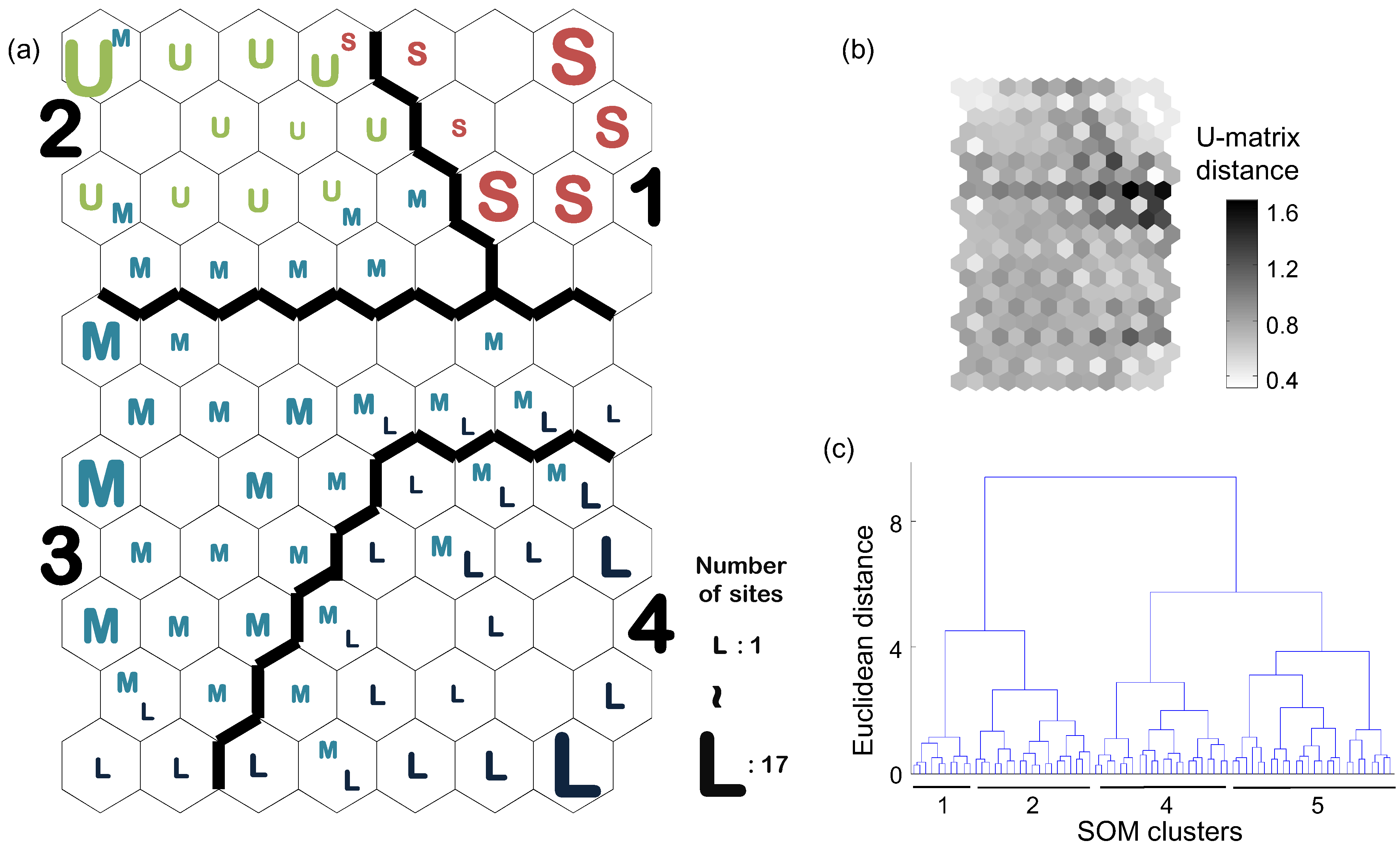
| Category Variable | SOM Cluster (number of study sites) | ||||
|---|---|---|---|---|---|
| 1 (51) | 2 (57) | 3 (69) | 4 (72) | ||
| Environmental Variable | Slope (m/km) | 51.0 (41.7)a | 2.5 (13.2)b | 0.6 (0.8)b | 0.1 (0.2)b |
| Current velocity (m/s) | 0.16 (0.14)a | 0.06 (0.1)b | 0.19 (0.2)a | 0.02 (0.04)b | |
| Width (m) | 0.7 (0.7)c | 2.4 (2.2)bc | 9.1 (8.5)b | 26 (27.3)a | |
| Depth (m) | 0.1 (0.1)c | 0.3 (0.2)c | 0.9 (0.7)b | 2.2 (1.5)a | |
| Emergent macrophytes (%) | 3.9 (11.1)c | 16.3 (22.1)ab | 8.5 (15.7)bc | 17.4 (22.0)a | |
| Floating macrophytes (%) | 0.0 (0.0)c | 8.3 (17.3)b | 3.9 (11.9)bc | 17.5 (20.2)a | |
| Submerged macrophytes (%) | 1.4 (7.5)b | 16.7 (19.1)a | 15.8 (25.4)a | 7.6 (15.2)b | |
| Detritus (%) | 40.8 (23.7)a | 3.5 (9.4)b | 6.5 (11.6)b | 2.3 (7.6)b | |
| Micro substrate (%) | 35.2 (20.5)a | 34.8 (22.5)a | 41.3 (25.3)a | 20.8 (14.2)b | |
| Macro substrate (%) | 10.2 (14.1)a | 0.8 (3.9)b | 2.2 (6.7)b | 0.9 (3.2)b | |
| pH | 6.77 (0.61)b | 6.8 (0.89)b | 7.28 (0.51)a | 7.54 (0.38)a | |
| Conductivity (μS/cm) | 259.5 (83.8)b | 486.5 (415.9)a | 524.9 (192.7)a | 559.3 (155.4)a | |
| DO (mg/L) | 8.67 (2.98)b | 9.92 (3.41)ab | 9.93 (2.08)ab | 10.86 (3.93)a | |
| NH4+ (mgN/L) | 0.16 (0.14)c | 2.57 (3.09)a | 1.55 (1.78)b | 0.83 (1.1)bc | |
| NO3− (mgN/L) | 11.86 (8.03)a | 5.59 (6.04)b | 8.55 (19.01)ab | 2.09 (1.62)c | |
| o-P (mgP/L) | 0.24 (0.56) | 0.51 (1.2) | 0.50 (0.73) | 0.20 (0.51) | |
| t-P (mgP/L) | 0.24 (0.25)b | 0.75 (1.68)ab | 0.87 (1.09)a | 0.42 (0.71)ab | |
| Cl− (mg/L) | 31.67 (13.77)b | 65.14 (101.1)a | 52.37 (64.73)ab | 59.49 (33.42)ab | |
| Ca2+ (mg/L) | 39.67 (18)c | 56.76 (33.4)b | 62.77 (20.07)ab | 68.75 (19.28)a | |
| Biological Index | Species richness | 28 (9)c | 37 (13)c | 59 (14)b | 83 (19)a |
| Shannon index | 3.06 (0.35)d | 3.31 (0.41)c | 3.85 (0.23)b | 4.21 (0.23)a | |
| Simpson index | 0.94 (0.02)b | 0.95 (0.03)b | 0.97 (0.01)a | 0.98 (0.00)a | |
| Evenness | 0.93 (0.02)c | 0.94 (0.02)b | 0.95 (0.01)a | 0.96 (0.01)a | |
| Exergy | 56206 (20399)c | 69393 (28168)c | 101275 (33297)b | 140525 (50483)a | |
| Specific exergy | 676 (25)b | 684 (34)b | 678 (20)b | 699 (22)a | |
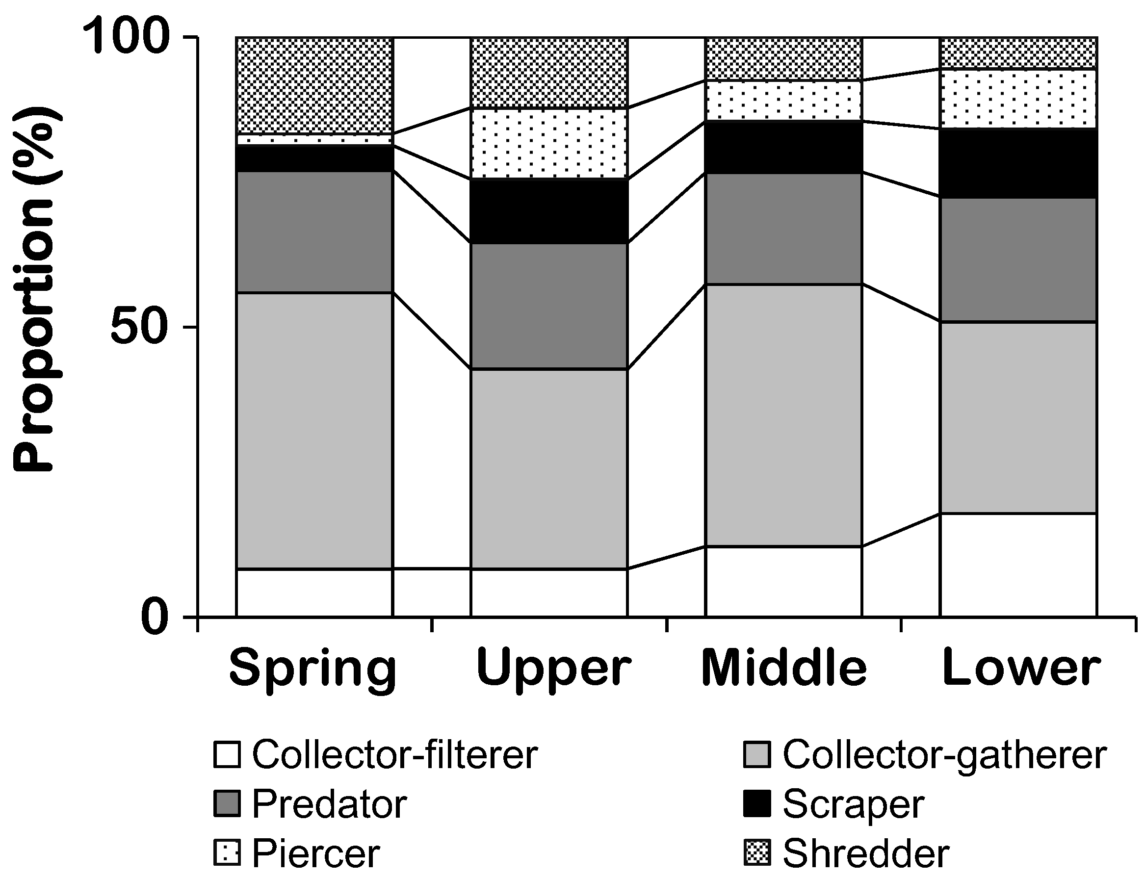
| Functional feeding group | Collector-filterers | 8.3 (5.7)c | 9.1 (6.4)c | 13.1 (5.3)b | 17.3 (5.7)a |
| Collector-gatherers | 47.6 (11.4)a | 36.2 (12.9)b | 43.9 (8.9)a | 34 (8.0)b | |
| Predators | 21.1 (8.4) | 20.9 (8.1) | 19.8 (5.6) | 21.5 (7) | |
| Piercers | 2.0 (2.5)c | 11.5 (7.0)ab | 7.6 (4.4)b | 9.7 (3.7)a | |
| Scrapers | 4.2 (3.3)c | 10.6 (7.6)a | 8.5 (5.4)b | 12.1 (3.9)a | |
| Shredders | 16.8 (8.6)a | 11.8 (7.6)a | 7.1 (2.9)b | 5.4 (1.9)b | |
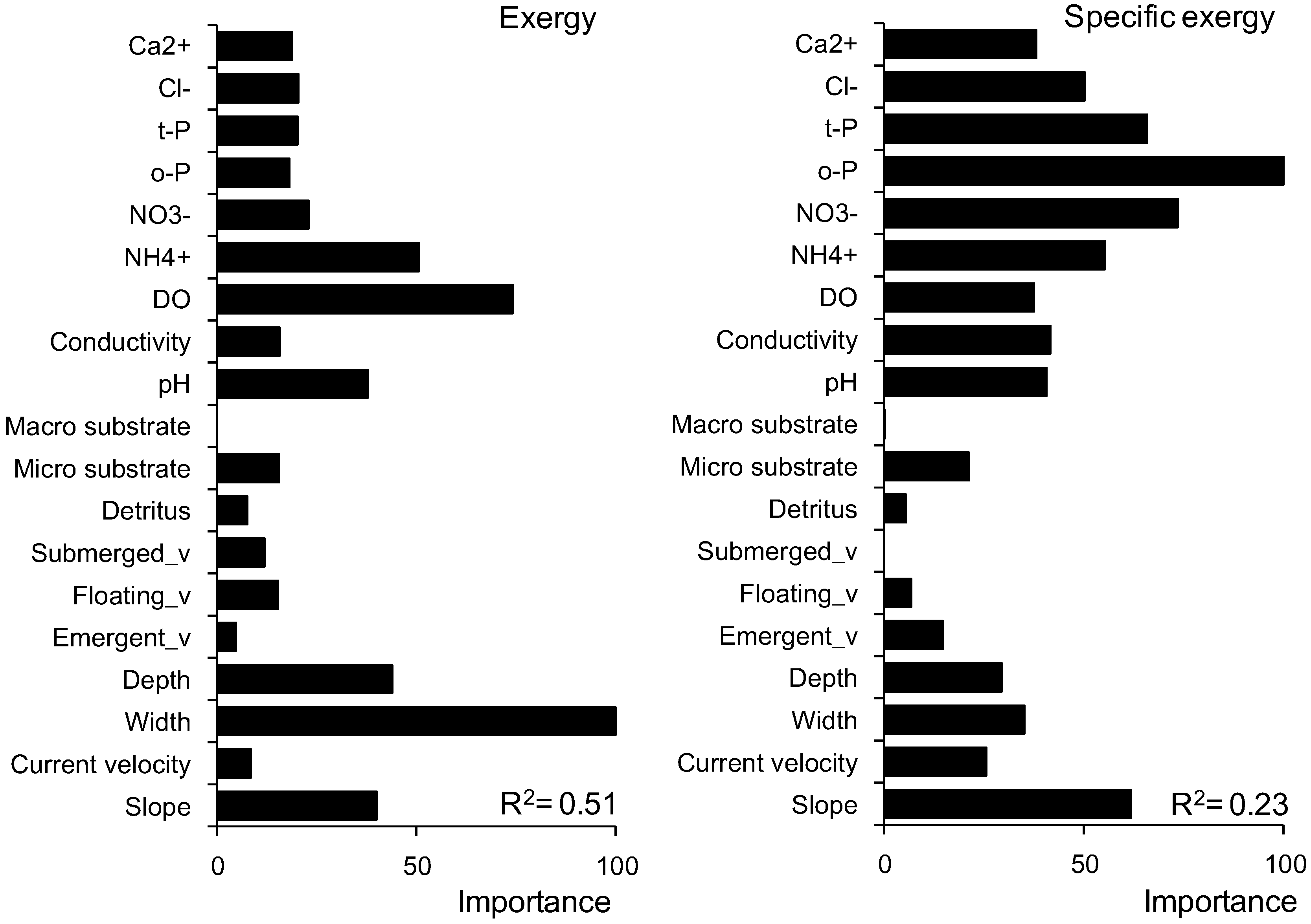
3.3. Prediction of Exergy

| Indices | Species Richness | Shannon Index | Simpson Index | Evenness | Exergy |
|---|---|---|---|---|---|
| Shannon index | 0.997** | ||||
| Simpson index | 0.992** | 0.998** | |||
| Evenness | 0.702** | 0.745** | 0.773** | ||
| Exergy | 0.919** | 0.911** | 0.912** | 0.589** | |
| Specific exergy | 0.299** | 0.316** | 0.320** | 0.316** | 0.267** |
4. Discussion
5. Conclusions
Acknowledgments
Conflict of Interest
Appendix
| Taxa | Indicator species | Cluster | IndVal | p |
|---|---|---|---|---|
| Ephemeroptera | Caenis horaria | 3 | 42 | 0.0001 |
| 4 | 43 | 0.0001 | ||
| Cloeon dipterum | 3 | 32 | 0.0001 | |
| 4 | 36 | 0.0001 | ||
| Caenis robusta | 4 | 32 | 0.0001 | |
| Cloeon simile | 4 | 32 | 0.0001 | |
| Chironomidae | Brillia modesta | 1 | 73 | 0.0001 |
| Micropsectra sp. | 1 | 60 | 0.0001 | |
| Polypedilum breviantennatum | 1 | 29 | 0.0001 | |
| Parametriocnemus stylatus | 1 | 27 | 0.0001 | |
| Macropelopia sp. | 1 | 27 | 0.0001 | |
| Psectrotanypus varius | 2 | 37 | 0.0001 | |
| Chironomus sp. | 2 | 33 | 0.0002 | |
| Xenopelopia nigricans | 2 | 26 | 0.0001 | |
| Natarsia sp. | 2 | 25 | 0.0001 | |
| Procladius sp. | 3 | 42 | 0.0001 | |
| 4 | 31 | 0.0001 | ||
| Cryptochironomus sp. | 3 | 37 | 0.0001 | |
| 4 | 35 | 0.0001 | ||
| Polypedilum gr. nubeculosum | 3 | 37 | 0.0001 | |
| 3 | 32 | 0.0001 | ||
| Conchapelopia sp. | 3 | 32 | 0.0001 | |
| Paratanytarsus sp. | 3 | 29 | 0.0001 | |
| Endochironomus albipennis | 4 | 85 | 0.0001 | |
| Polypedilum gr. Sordens | 4 | 62 | 0.0001 | |
| Glyptotendipes sp. | 4 | 62 | 0.0001 | |
| Cricotopus sp. | 4 | 55 | 0.0001 | |
| Endochironomus tendens | 4 | 49 | 0.0001 | |
| Dicrotendipes gr. nervosus | 4 | 45 | 0.0001 | |
| Parachironomus gr. arcuatus | 4 | 45 | 0.0001 | |
| Microtendipes sp. | 4 | 33 | 0.0001 | |
| Ablabesmyia longistyla | 4 | 32 | 0.0001 | |
| Cladotanytarsus sp. | 4 | 30 | 0.0001 | |
| Tanytarsus sp. | 4 | 29 | 0.0001 | |
| Clinotanypus sp rvosus | 4 | 28 | 0.0001 | |
| Corynoneura sp. | 4 | 26 | 0.0001 | |
| Plecoptera | Nemoura cinerea | 1 | 29 | 0.0001 |
| Nemurella pictetii | 1 | 27 | 0.0001 | |
| Tricoptera | Plectrocnemia conspersa | 1 | 74 | 0.0001 |
| Stenophylax sp. | 1 | 47 | 0.0001 | |
| Sericostoma personatum | 1 | 41 | 0.0001 | |
| Beraea Maura | 1 | 35 | 0.0001 | |
| Athripsodes aterrimus | 3 | 31 | 0.0001 | |
| Mystacides sp. | 4 | 47 | 0.0001 | |
| Cyrnus flavidus | 4 | 45 | 0.0001 | |
| Triaenodes bicolor | 4 | 33 | 0.0001 | |
| Ecnomus tenellus | 4 | 29 | 0.0001 | |
| Dipetera | Hexatominae | 1 | 63 | 0.0001 |
| Ptychoptera sp. | 1 | 51 | 0.0001 | |
| Pedicia sp. | 1 | 45 | 0.0001 | |
| Dicranota bimaculata | 1 | 45 | 0.0001 | |
| Dixa maculate | 1 | 41 | 0.0001 | |
| Tipula sp. | 1 | 34 | 0.0001 | |
| Ceratopogonidae | 3 | 26 | 0.0088 | |
| Coleoptera | Elodes minuta | 1 | 82 | 0.0001 |
| Hydrobius fuscipes | 2 | 42 | 0.0001 | |
| Hydroporus palustris | 2 | 41 | 0.0001 | |
| Haliplus lineatocollis | 2 | 28 | 0.0001 | |
| Agabus sp./Ilybius sp. | 2 | 27 | 0.0002 | |
| Haliplus fluviatilis | 4 | 30 | 0.0001 | |
| Hygrotus versicolor | 4 | 30 | 0.0001 | |
| Noterus clavicornis | 4 | 28 | 0.0001 | |
| Laccophilus hyalinus | 4 | 28 | 0.0001 | |
| Haliplus sp. | 4 | 27 | 0.0002 | |
| Odonata | Ischnura sp. | 4 | 40 | 0.0001 |
| Hemiptera | Sigara fallen | 4 | 53 | 0.0001 |
| Sigara striata | 4 | 39 | 0.0001 | |
| Sigara distincta/falleni/longipalis | 4 | 34 | 0.0001 | |
| Ilyocoris cimicoides | 4 | 30 | 0.0001 | |
| Hirudinea | Erpobdella octoculata | 3 | 42 | 0.0001 |
| Glossiphonia complanata | 3 | 28 | 0.0001 | |
| Helobdella stagnalis | 4 | 51 | 0.0001 | |
| Glossiphonia heteroclite | 4 | 44 | 0.0001 | |
| Hemiclepsis marginata | 4 | 44 | 0.0001 | |
| Piscicola geometra | 4 | 30 | 0.0001 | |
| Amphipoda | Gammarus pulex | 1 | 58 | 0.0001 |
| Asellus aquaticus | 4 | 30 | 0.0001 | |
| Proasellus coxalis | 4 | 29 | 0.0001 | |
| Bivalva | Sphaerium sp. | 3 | 34 | 0.0001 |
| Actinedida | Sperchon squamosus | 1 | 35 | 0.0001 |
| Limnesia koenikei | 3 | 33 | 0.0001 | |
| Hygrobates longipalpis | 3 | 32 | 0.0001 | |
| Hygrobates nigromaculatus | 3 | 23 | 0.0001 | |
| Limnesia maculate | 4 | 70 | 0.0001 | |
| Piona alpicola/coccinea | 4 | 60 | 0.0001 | |
| Arrenurus crassicaudatus | 4 | 54 | 0.0001 | |
| Limnesia undulate | 4 | 52 | 0.0001 | |
| Mideopsis orbicularis | 4 | 40 | 0.0001 | |
| Acercinae | 4 | 38 | 0.0001 | |
| Piona pusilla | 4 | 33 | 0.0001 | |
| Unionicola crassipes | 4 | 32 | 0.0001 | |
| Piona variabilis | 4 | 31 | 0.0001 | |
| Limnesia sp | 4 | 29 | 0.0001 | |
| Arrenurus globator | 4 | 28 | 0.0001 | |
| Eylais extendens | 4 | 27 | 0.0001 | |
| Oligochaeta | Eiseniella tetraedra | 1 | 32 | 0.0001 |
| Enchytraeidae | 1 | 26 | 0.0001 | |
| Lumbriculus variegatus | 2 | 27 | 0.0151 | |
| Tubificidae sp.1 | 3 | 34 | 0.0001 | |
| 4 | 33 | 0.0001 | ||
| Tubificidae sp.2 | 3 | 34 | 0.0001 | |
| Stylaria lacustris | 4 | 44 | 0.0001 | |
| Ophidonais serpentine | 4 | 35 | 0.0001 | |
| Potamothrix hammoniensis | 4 | 29 | 0.0001 | |
| Limnodrilus hoffmeisteri | 3 | 28 | 0.0004 | |
| 4 | 29 | 0.0004 | ||
| Potamothrix moldaviensis | 4 | 26 | 0.0001 | |
| Gastropoda | Anisus leucostoma/spirorbis | 2 | 40 | 0.0001 |
| Radix peregra | 2 | 31 | 0.0001 | |
| Bithynia leachi | 4 | 63 | 0.0001 | |
| Bithynia tentaculata | 4 | 58 | 0.0001 | |
| Valvata piscinalis | 4 | 54 | 0.0001 | |
| Anisus vortex | 4 | 53 | 0.0001 | |
| Gyraulus albus | 4 | 47 | 0.0001 | |
| Valvata cristata | 4 | 39 | 0.0001 | |
| Physa fontinalis | 4 | 34 | 0.0001 | |
| Acroloxus lacustris | 4 | 32 | 0.0001 |
References
- Odum, E.P. Ecological potential and analogue circuits for the ecosystem. Am. Sci. 1960, 48, 1–8. [Google Scholar]
- Margalef, R. Communication of structure in plankton population. Limnol. Oceanogr. 1961, 6, 124–128. [Google Scholar] [CrossRef]
- Straskraba, M. Cybernetic categories of ecosystem dynamics. ISEM J. 1980, 2, 81–96. [Google Scholar]
- Odum, H.T. Pulsing, power and hierarchy. In Energetics and Systems; Mitsh, W.J., Ragade, R.K., Bosserman, R.W., Dillon, J.A., Jr., Eds.; Ann Arbor Science: Ann Arbor, MI, USA, 1982; pp. 33–59. [Google Scholar]
- Jørgensen, S.E. Exergy and Buffering Capacity in Ecological System. In Energetics and Systems; Mitsh, W.J., Ragade, R.K., Bosserman, R.W., Dillon, J.A., Jr., Eds.; Ann Arbor Science: Ann Arbor, MI, USA, 1982; pp. 61–72. [Google Scholar]
- Ulanowicz, R.E. Growth and Development: Ecosystem Phenomenology; Springer: New York, NY, USA, 1986. [Google Scholar]
- Schneider, E. Thermodynamics, ecological succession, and natural selection: A common thread. In Entropy, Information and Evolution; Weber, B.H., Depew, D.J., Smith, J.D., Eds.; MIT Press: Cambridge, MA, USA, 1988. [Google Scholar]
- Xu, F.L.; Jørgensen, S.E.; Tao, S.; Li, B.G. Modeling the effects of ecological engineering on ecosystem health of a shallow eutrophic Chinese lake (Lake Chao). Ecol. Model. 1999, 117, 239–260. [Google Scholar] [CrossRef]
- Silow, E.A.; Oh, I.H. Aquatic ecosystem assessment using exergy. Ecol. Indic. 2004, 4, 189–198. [Google Scholar] [CrossRef]
- Silow, E.A.; Mokry, A.V. Exergy as a tool for ecosystem health assessment. Entropy 2010, 12, 902–925. [Google Scholar] [CrossRef]
- Mandal, S.; Ray, S.; Jørgensen, S.E. Exergy as an indicator: Observations of an aquatic ecosystem model. Ecol. Inform. 2012, 12, 1–9. [Google Scholar] [CrossRef]
- Li, F.; Bae, M.J.; Kwon, Y.S.; Chung, N.; Hwang, S.J.; Park, S.J.; Park, H.K.; Kong, D.S.; Park, Y.S. Ecological exergy as an indicator of land-use impacts on functional guilds in river ecosystems. Ecol. Model. 2013, 252, 53–62. [Google Scholar] [CrossRef]
- Jørgensen, S.E.; Mejer, H. Ecological buffer capacity. Ecol. Model. 1977, 3, 39–61. [Google Scholar] [CrossRef]
- Jørgensen, S.E.; Mejer, H. A holistic approach to ecological modelling. Ecol. Model. 1979, 7, 169–189. [Google Scholar] [CrossRef]
- Xu, F.L.; Tao, S.; Dawson, R.W. System-level responses of lake ecosystems to chemical stresses using exergy and structural exergy as ecological indicators. Chemosphere 2002, 46, 173–185. [Google Scholar] [CrossRef]
- Park, Y.S.; Lek, S.; Scardi, M.; Verdonschot, P.F.M.; Jørgensen, S.E. Patterning exergy of benthic macroinvertebrate communities using self-organizing maps. Ecol. Model. 2006, 195, 105–113. [Google Scholar] [CrossRef] [Green Version]
- Jørgensen, S.E.; Nielsen, S.N. Application of exergy as thermodynamic indicator in ecology. Energy 2007, 32, 673–685. [Google Scholar] [CrossRef]
- Fonseca, J.C.; Pardal, M.A.; Azeiteiro, U.M.; Marques, J.C. Estimation of ecological exergy using weighing parameters determined from DNA contents of organisms—A case study. Hydrobiologia 2002, 475, 79–90. [Google Scholar] [CrossRef]
- Mandal, S.; Ray, S.; Roy, S.; Mandal, S. The Concept of Exergy and its Extension to Ecological System. In Handbook of Exergy, Hydrogen Energy and Hydropower Research; Pélissier, G., Calvet, A., Eds.; Nova Science: New York, NY, USA, 2009; Chapter 13. [Google Scholar]
- Ludovisi, A.; Poletti, A. Use of thermodynamic indices as ecological indicators of the development state of lake ecosystems: 2. Exergy and specific exergy indices. Ecol. Model. 2003, 159, 223–238. [Google Scholar] [CrossRef]
- Jørgensen, S.E. Integration of Ecosystem Theories: A Pattern; 3nd revised ed.; Kluwer Academic Publishers: Boston, MA, USA, 2002. [Google Scholar]
- Jørgensen, S.E. Review and comparison of goal functions in system ecology. Vie et Milieu 1994, 44, 11–20. [Google Scholar]
- Xu, F.L.; Jørgensen, S.E.; Tao, S. Ecological indicators for assessing freshwater ecosystem health. Ecol. Model. 1999, 116, 77–106. [Google Scholar] [CrossRef]
- Jørgensen, S.E. The application of ecological indicators to assess the ecological condition of a lake. Lakes Reserv.: Res. Manag. 1995, 1, 177–182. [Google Scholar] [CrossRef]
- Bae, M.J.; Park, Y.S. Characterizing ecological exergy as an ecosystem indicator in streams using a self-organizing map. Korean J. Environ. Biol. 2008, 26, 203–213. [Google Scholar]
- Xu, F.-L.; Wang, J.-J.; Chen, B.; Qin, N.; Wu, W.W.; He, W.; He, Q.S.; Wang, Y. The variations of exergies and structural exergies along eutrophication gradients in Chinese and Italian lakes. Ecol. Model. 2011, 222, 337–350. [Google Scholar] [CrossRef]
- Marques, J.C.; Pardal, M.Â.; Nielsen, S.N.; Jørgensen, S.E. Analysis of the properties of exergy and biodiversity along an estuarine gradient of eutrophication. Ecol. Model. 1997, 102, 155–167. [Google Scholar] [CrossRef]
- Marques, J.C.; Nielsen, S.N.; Pardal, M.A.; Jørgensen, S.E. Impact of eutrophication and river management within a framework of ecosystem theories. Ecol. Model. 2003, 166, 147–168. [Google Scholar] [CrossRef]
- Fabiano, M.; Vassalo, P.; Vezzulli, L.; Salvo, V.S.; Marques, J.C. Temporal and spatial change of exergy and ascendency in different benthic marine ecosystems. Energy 2004, 29, 1697–1712. [Google Scholar] [CrossRef]
- Pranovi, F.; Da Ponte, F.; Torricelli, P. Application of biotic indices and relationship with structural and functional features of macrobenthic community in the lagoon of Venice: An example over a long time series of data. Mar. Pollut. Bull. 2007, 54, 1607–1618. [Google Scholar] [CrossRef] [PubMed]
- Wallace, J.B.; Webster, J.R. The role of macroinvertebrates in stream ecosystem function. Annu. Rev. Entomol. 1996, 41, 115–139. [Google Scholar] [CrossRef] [PubMed]
- Covich, A.P.; Palmer, M.A.; Crowl, T.A. The role of benthic invertebrate species in freshwater ecosystems. BioScience 1999, 49, 119–127. [Google Scholar] [CrossRef]
- Rosenberg, D.M.; Resh, V.H. Freshwater Biomonitoring and Benthic Macroinvertebrates; Chapman & Hall: London, UK, 1993; p. 325. [Google Scholar]
- Libralato, S.; Torricelli, P.; Pranovi, F. Exergy as ecosystem indicator: An application to the recovery process of marine benthic communities. Ecol. model. 2006, 192, 571–585. [Google Scholar] [CrossRef]
- Gessner, M.O.; Chauvet, E. A case for using litter breakdown to assess functional stream integrity. Ecol. Appl. 2002, 12, 498–510. [Google Scholar] [CrossRef]
- Bunn, S.E.; Mosisch, T.D.; Davies, P.M. Ecosystem measures of river health and their response to riparian and catchment degradation. Freshwater Biol. 1999, 41, 333–345. [Google Scholar] [CrossRef]
- McKie, B.G.; Malmqvist, B. Assessing ecosystem functioning in streams affected by forest management: increased leaf decomposition occurs without changes to the composition of benthic assemblages. Freshwater Biol. 2009, 54, 2086–2100. [Google Scholar] [CrossRef]
- Riipinen, M.P.; Davy-Bowker, J.; Dobson, M. Comparison of structural and functional stream assessment methods to detect changes in riparian vegetation and water pH. Freshwater Biol. 2009, 54, 2127–2138. [Google Scholar] [CrossRef]
- Stephenson, J.M.; Morin, A. Covariation of stream community structure and biomass of algae, invertebrates and fish with forest cover at multiple spatial scales. Freshwater Biol. 2009, 54, 2139–2154. [Google Scholar] [CrossRef]
- Ferreira, V.; Graca, M.A.S.; de Lima, J.; Gomes, R. Role of physical fragmentation and invertebrate activity in the breakdown rate of leaves. Arch. Hydrobiol. 2006, 165, 493–513. [Google Scholar] [CrossRef]
- Death, R.G.; Dewson, Z.S.; James, A.B.W. Is structure or function a better measure of the effects of water abstraction on ecosystem integrity? Freshwater Biol. 2009, 54, 2037–2050. [Google Scholar] [CrossRef]
- Friberg, N.; Dybkjær, J.B.; Olafsson, J.S.; Gislason, G.M.; Larsen, S.E.; Lauridsen, T.L. Relationships between structure and function in streams contrasting in temperature. Freshwater Biol. 2009, 54, 2051–2068. [Google Scholar] [CrossRef]
- Bird, G.A.; Kaushik, N.K. Invertebrate colonization and processing of maple leaf litter in a forested and an agricultural reach of a stream. Hydrobiologia 1992, 234, 65–77. [Google Scholar] [CrossRef]
- Gücker, B.; Boüchat, I.G.; Giani, A. Impacts of agricultural land use on ecosystem structure and whole-stream metabolism of tropical Cerrado streams. Freshwater Biol. 2009, 54, 2069–2085. [Google Scholar] [CrossRef]
- Young, R.G.; Collier, K.J. Contrasting responses to catchment modification among a range of functional and structural indicators of river ecosystem health. Freshwater Biol. 2009, 54, 2155–2170. [Google Scholar] [CrossRef]
- Sandin, L.; Solimini, A.G. Freshwater ecosystem structure-function relationships: from theory to application. Freshwater Biol. 2009, 54, 2017–2024. [Google Scholar] [CrossRef]
- Verdonschot, P.F.M.; Nijboer, R.C. Typology of Macrofaunal assemblages applied to water and nature management: A Dutch approach. In Assessing the Biological Quality of Fresh Waters: RIVPACS and Other Techniques; Wright, J.F., Sutcliffe, D.W., Furse, M.T., Eds.; The Freshwater Biological Association: Ambleside, Cumbria, UK, 2000; pp. 241–262. [Google Scholar]
- Tomanova, S.; Goitia, E.; Helešic, J. Trophic levels and functional feeding groups of macroinvertebrates in Neotropical streams. Hydrobiologia 2006, 556, 251–264. [Google Scholar] [CrossRef]
- Cummins, K.W. Invertebrates. In The Rivers Handbook; Calow, P., Petts, G.E., Eds.; Blackwell Scientific: Oxford, UK, 1995; pp. 234–250. [Google Scholar]
- Mihuc, T.B. The functional trophic role of lotic primary consumers: generalist versus specialist strategies. Freshwater Biol. 1997, 37, 455–462. [Google Scholar] [CrossRef]
- Merritt, R.W.; Cummins, K.W.; Berg, M.B. An Introduction to the Aquatic Insects of North America, 4th revised ed; Hunt Publishing Company: Dubugue, IA, USA, 2006. [Google Scholar]
- Verdonschot, P.F.M. Typology of macrofaunal assemblages: A tool for the management of running waters in The Netherlands. Hydrobiologia 1995, 297, 99–122. [Google Scholar] [CrossRef]
- Austoni, M.; Giordani, G.; Viaroli, P.; Zaldívar, J.M. Application of specific exergy to macrophytes as an integrated index of environmental quality for coastal lagoons. Ecol Indic. 2007, 7, 229–238. [Google Scholar] [CrossRef]
- Jørgensen, S.E.; Nielsen, S.N. Thermodynamic orientors: Exergy as a Goal Function in Ecological Modeling and as an Ecological Indicator for the Description of Ecosystem Development. In Eco Targets, Goal Functions, and Orientors; Müller, F., Leupelt, M., Eds.; Springer: Berlin, Germany, 1998; pp. 63–86. [Google Scholar]
- Jørgensen, S.E.; Nielsen, S.N.; Mejer, H. Emergy, environ, exergy and ecological modelling. Ecol. Model. 1995, 77, 99–109. [Google Scholar] [CrossRef]
- Jørgensen, S.E.; Verdonschot, P.; Lek, S. Explanation of the observed structure of functional feeding groups of aquatic macro-invertebrates by an ecological model and the maximum exergy principle. Ecol. Model. 2002, 158, 223–231. [Google Scholar] [CrossRef]
- Kohonen, T. Self-organized formation of topologically correct feature maps. Biol. Cybern. 1982, 42, 59–69. [Google Scholar] [CrossRef]
- Kohonen, T. Self-Organizing Maps, 3rd ed.; Springer: Berlin, Germany, 2001. [Google Scholar]
- Park, Y.S.; Chang, J.; Lek, S.; Cao, W.; Brosse, S. Conservation strategies for endemic fish species threatened by the Three Gorges Dam. Conser. Biol. 2003, 17, 1748–1785. [Google Scholar] [CrossRef]
- Alhoniemi, E.; Himberg, J.; Parhankangas, J.; Vesanto, J. SOM Toolbox; Laboratory of Information and Computer Science, Helsinki University of Technology: Helsinki, Finland, 2000; Available online: http://www.cis.hut.fi/projects/somtoolbox/ (accessed on 31/03/2012).
- MATLAB; Version 6.1; software for technical computation; The Mathworks Inc.: Natick, MA, USA, 2001.
- Ultsch, A. Self-Organizing Neural Networks for Visualization and Classification. In Information and Classification; Opitz, O., Lausen, B., Klar, R., Eds.; Springer: Berlin, Germany, 1993; pp. 307–313. [Google Scholar]
- Ward, J.H. Hierarchical grouping to optimize an objective function. J. Am. Stat. Assoc. 1963, 58, 236–244. [Google Scholar] [CrossRef]
- Jain, A.K.; Dubes, R.C. Algorithms for Clustering Data; Prentice Hall: Englewood Cliffs, NJ, USA, 1988. [Google Scholar]
- McCune, B.; Mefford, M.J. PC-ORD; Multivariate Analysis of Ecological Data; MjM Software Design: Glenden Beach, OR, USA, 1999. [Google Scholar]
- Dufrene, M.; Legendre, P. Species assemblages and indicator species: The need for a flexible asymmetrical approach. Ecol. Mono. 1997, 67, 345–366. [Google Scholar] [CrossRef]
- Chaves, M.L.; Rieradevall, M.; Chainho, P.; Costa, J.L.; Costa, M.J.; Prat, N. Macroinvertebrate communities of non-glacial high altitude intermittent streams. Freshwater Biol. 2008, 53, 55–76. [Google Scholar] [CrossRef]
- García-Roger, E.; Sánchez-Montoya, M.M.; Gomez, R.; Suárez, M.L.; Vidal-Abarca, M.R.; Latron, J.; Rieradevall, M.; Prat, N. Do seasonal changes in habitat features influence aquatic macroinvertebrate assemblages in perennial versus temporary Mediterranean streams? Aquat. Sci. 2011, 73, 567–579. [Google Scholar] [CrossRef]
- Breiman, L. Random forests. Mach. Learn. 2001, 45, 5–32. [Google Scholar] [CrossRef]
- Zar, J. Biostatistical Analysis, 4th ed.; Prentice-Hall: Upper Saddle River, NJ, USA, 1999. [Google Scholar]
- STATISTICA; Version 7; data analysis software system; StatSoft Inc.: Tulsa, OK, USA, 2004; Available online: http://www.statsoft.com (accessed on 31/03/2012).
- Schneider, E.D.; Kay, J.J. Life as a manifestation of the second law of thermodynamics. Math. Comp. Model. 1994, 9, 25–48. [Google Scholar] [CrossRef]
- Spieles, D.J.; Mitsch, W.J. A model of macroinvertebrate trophic structure and oxygen demand in freshwater wetlands. Ecol. Model. 2003, 161, 183–194. [Google Scholar] [CrossRef]
- Park, Y.S.; Kwak, I.S.; Chon, T.S.; Kim, J.K.; Jørgensen, S.E. Implementation of artificial neural networks in patterning and prediction of exergy in response to temporal dynamics of benthic macroinvertebrate communities in streams. Ecol. Model. 2001, 146, 143–157. [Google Scholar] [CrossRef]
- de Wit, R.; Stal, L.J.; Lomstein, B.A.; Herbert, R.A.; van Gemerden, H.; Viaroli, P.; Ceccherelli, V.U.; Rodriguez-Valera, F.; Bartoli, M.; Giordani, G.; et al. Robust: The role of buffering capacities in stabilising coastal lagoon ecosystems. Cont. Shelf Res. 2001, 21, 2021–2041. [Google Scholar] [CrossRef]
- Verdonschot, P.F.M. Ecological Characterization of Surface Waters in the Province of Overijssel, The Netherlands. Ph.D. Thesis, Agriculture University of Wageningen, Wageningen, The Netherlands, 1990. [Google Scholar]
- Molozzi, J.; Salas, F.; Callisto, M.; Marques, J.C. Thermodynamic oriented ecological indicators: Application of Eco-Exergy and specific Eco-Exergy in capturing environmental changes between disturbed and non-disturbed tropical reservoirs. Ecol. Indi. 2013, 24, 543–551. [Google Scholar] [CrossRef]
© 2013 by the authors; licensee MDPI, Basel, Switzerland. This article is an open access article distributed under the terms and conditions of the Creative Commons Attribution license (http://creativecommons.org/licenses/by/3.0/).
Share and Cite
Bae, M.-J.; Li, F.; Verdonschot, P.F.M.; Park, Y.-S. Characterization of Ecological Exergy Based on Benthic Macroinvertebrates in Lotic Ecosystems. Entropy 2013, 15, 2319-2339. https://doi.org/10.3390/e15062319
Bae M-J, Li F, Verdonschot PFM, Park Y-S. Characterization of Ecological Exergy Based on Benthic Macroinvertebrates in Lotic Ecosystems. Entropy. 2013; 15(6):2319-2339. https://doi.org/10.3390/e15062319
Chicago/Turabian StyleBae, Mi-Jung, Fengqing Li, Piet F.M. Verdonschot, and Young-Seuk Park. 2013. "Characterization of Ecological Exergy Based on Benthic Macroinvertebrates in Lotic Ecosystems" Entropy 15, no. 6: 2319-2339. https://doi.org/10.3390/e15062319