Effect of Prey Refuge on the Spatiotemporal Dynamics of a Modified Leslie-Gower Predator-Prey System with Holling Type III Schemes

Abstract

In this paper, the spatiotemporal dynamics of a diffusive Leslie-Gower predator-prey model with prey refuge are investigated analytically and numerically. Mathematical theoretical works have considered the existence of global solutions, population permanence and the stability of equilibrium points, which depict the threshold expressions of some critical parameters. Numerical simulations are performed to explore the pattern formation of species. These results show that the prey refuge has a profound effect on predator-prey interactions and they have the potential to be useful for the study of the entropy theory of bioinformatics.

1. Introduction

The dynamic relationship between predators and their prey has fascinated mathematical biologists for a long time. A variety of mathematical models are devoted to exploring the predator-prey interaction [1,2,3,4]. To understand well the population dynamics, many biological factors are included such as time delay, impulsive effect, seasonal perturbation [5,6,7,8,9]. Recently, many authors [10,11] have focused on the dynamics of a class of the semi-ratio-dependent predator-prey models, in which one of the salient features is that the carrying capacity of predator is proportional to the number of prey and such models were initially introduced by Leslie and Gower [12,13]. In 2003, Aziz-Alaoui and Okiye [14] analyzed the dynamics of the following model:

(1)

where u and w represent the densities of prey and predator, respectively. Furthermore, it is assumed that the prey grows logistically with the limited factor k of considering realistic surroundings and innate growth rate r. In Equation (1), k₁ is the average saturation rate, which indicates the quality of the food that provides prey to predator, k₂ indicates the quality of the alternative that provides the environment, s is the intrinsic growth rate of predator, e is the maximum reduction of prey due to predation and h measures the ration of prey to support one predator. Here the functional response of predator is Holling type II schemes, which usually depicts the uptake of substrate by the microorganisms in microbial kinetics [15]. Oftentimes Holling type III schemes is used to describe the dynamical behavior of the invertebrate feeding on the prey and this functional response of predator has been widely included in mathematic ecological models [16,17,18,19]. In fact, if the predator is the invertebrate, Holling type III functional response can fit better [20]. On the other hand, the effect of a constant proportion of prey refuge on predator-prey models has become a pretty hot issue in mathematical ecology in the recent years. By investigating the theoretical models, most of theoretical conclusions show that the prey refuge has a stabilizing effect on predator-prey systems, but the dynamics of the Kolmogorov type model incorporating a constant proportion of prey refuge is qualitatively equivalent to the original system [21,22,23,24,25,26]. Thus, we consider the following system:

(2)

where $m(m\in [0,1))$ is a constant and $(1-m)u$ reflects the prey available to the predator, $\sqrt{a}$ is the half-saturation constant for the predator and b indicates the quality of the alternative that provides the environment.

On the other hand, all living beings live in a spatial world, which can cause that the spatial component of ecological interactions exhibits ranging from individual behavior to species abundance, diversity and population dynamics. Therefore, the spatial factor is one of the most important elements in ecosystem. Lately, Camera [27] has specified the spatiotemporal dynamics of Equation (1) with diffusion of species. Meanwhile, a large amount of literatures mainly study this theme in reaction-diffusion systems since Turing [28] pointed out that this kind of system could yield many complex patterns, which are usually consistent with a wide variety of phenomena that have been observed in chemistry, physics and biology [29,30,31]. Thus, Equation (2) with the spatial factor can be described as following:

(3)

where $u(t,x)$ and $w(t,x)$ denote the densities of prey and predator at time t and position x, respectively. Δ is the Laplacian operator, $d_1$ and $d_2$ are the diffusion coefficients of prey and predator, and $\frac{\partial }{\partial n}$ is differentiation in the direction of the outward unit normal to $\partial \text{Ω}$. In Equation (3), all the parameters are assumed to be positive.

The rests of the paper are structured as follows: in Section 2, the existence of the global solutions and the population permanence of Equation (3) are proved. In Section 3, the local stability of the equilibrium points and the global stability of the interior equilibrium point are investigated. Furthermore, the Turing instability and the conditions of its occurrence are analyzed. In Section 4, under the condition of Turing instability, numerical simulations are illustrated to show how the prey refuge affects spatiotemporal dynamics of Equation (3). In the end, some discussions are given.

2. Existence of Global Solutions and Permanence

2.1. Existence of Global Solutions

Theorem 1.

For $u_0(x)\ge 0$, $w_0(x)\ge 0$, there is a unique global solution of Equation (3) such that $u(t,x)>0$, $w(t,x)>0$ for $t>0$ and $x\in \overline{\text{Ω}}$.

Proof:

Equation (3) is mixed quasi-monotone since:

(4)

(5)

in ${R_{+}}^2=\{u\ge 0,w\ge 0\}$.

Consider that $(\widehat{u},\widehat{w})$ is the unique solution of:

(6)

where $u^{*}={\sup }_{\overline{\text{Ω}}}{u}_0(x)$, $w^{*}={\sup }_{\overline{\text{Ω}}}{w}_0(x)$.

Let $(\underset{\_}{u}(t,x),\underset{\_}{w}(t,x))=(0,0)$ and $(\overline{u}(t,x),\overline{w}(t,x))=(\widehat{u},\widehat{w})$. There exist:

(7)

(8)

Clearly, the boundary conditions are satisfied. Then $(\underset{\_}{u}(t,x),\underset{\_}{w}(t,x))$ and $(\overline{u}(t,x),\overline{w}(t,x))$ are the lower-solution and upper-solution of Equation (3), respectively. Thus, Equation (3) has a unique global solution, which can satisfy $0\le u(t,x)\le \widehat{u}(t)$, $0\le w(t,x)\le \widehat{w}(t)$ for $t\ge 0$.

2.2. Permanence

Definition 1. Equation (3) is said to be permanence if for any solution with nonnegative initial functions $u_0(x)$ and $w_0(x)$$(u_0(x)\ne 0,w_0(x)\ne 0)$, there exist positive constants $m_i$ and $M_i$ ($i=1,2$) such that:

(9)

(10)

Theorem 2.

For any solution $(u(t,x),w(t,x))$ of Equation (3):

(11)

Proof:

Suppose that $(u(t,x),w(t,x))$ is any solution of Equation (3), then there is:

(12)

Furthermore, it is assumed that $\stackrel{⌢}{U}(t)$ is any solution of:

(13)

then there is $\underset{t\to \infty }{\lim }\stackrel{⌢}{U}(t)=k$. By the comparison principle, there exists $\underset{t\to \infty }{\lim \sup }u(t,x)\le k$. As a consequence, for any $\epsilon >0$, there exists $T>0$ such that $u(t,x)\le k+\epsilon$ for $t>T$. Then there is:

(14)

Consider that $\stackrel{⌢}{W}(t)$ is any solution of:

(15)

then it leads to $\underset{t\to \infty }{\lim }\stackrel{⌢}{W}(t)\le \frac{b+(1-m)(k+\epsilon )}{h}$.

Similarly, there exists $\underset{t\to \infty }{\lim \sup }w(t,x)\le \frac{b+(1-m)(k+\epsilon )}{h}$.

As a result, let $\epsilon \to 0$, it has $\underset{t\to \infty }{\lim \sup }w(t,x)\le \frac{b+k(1-m)}{h}$. This completes the proof.

Theorem 3.

Assume that $hr>e{(1-m)}^{2}k(b+k(1-m))$, then:

(16)

where $\eta =1-\frac{ea{(1-m)}^{2}k(b+k(1-m))}{ahr}$.

Proof:

Assume that $(u,w)$ is any solution of Equation (3) with $u_0(x)\ge 0$ and $w_0(x)\ge 0$ $(u_0(x)\ne 0,w_0(x)\ne 0)$. Meanwhile, there is $u(t,x)\ge 0$ for all $t\ge 0$. Then there is $1-\frac{hw}{b+(1-m)u}\ge 1-\frac{hw}{b}$ for all $t\ge 0$, $x\in \overline{\text{Ω}}$. Assume that $w(T_1,x)>0$ for $T_1>0$. Consider that $\stackrel{⌣}{W}$ is any solution of:

(17)

then it has $\underset{t\to \infty }{\lim }\stackrel{⌣}{W}(t)=\frac{b}{h}$. By the comparison principle, there is $\underset{t\to \infty }{\lim \inf }w(t,x)\ge \frac{b}{h}>0$ for $x\in \overline{\text{Ω}}$. By Theorems 1 and 2, there exists $T_2>0$ such that:

(18)

for $t\ge T_2,x\in \overline{\text{Ω}}$.

Let $\eta =1-\frac{ea{(1-m)}^{2}k(b+k(1-m))}{ahr}$. Consider that $\stackrel{⌣}{U}(t)$ is any solution of:

(19)

then it has $\underset{t\to \infty }{\lim }\stackrel{⌣}{U}(t)=k\eta$. Similarly, there is $\underset{t\to \infty }{\lim \inf }u(t,x)\ge k\eta$. According to the assumption in the theorem, it can yield $\underset{t\to \infty }{\lim \inf }u(t,x)\ge k\eta >0$. This completes the proof.

Remark 1. From Theorem 2 and Theorem 3, it is clear that Equation (3) is permanent.

3. Stability Analysis of Equilibrium Points and Turing Instability

3.1. Stability

It is clear that Equation (3) has the following equilibrium points: (a) $E_0=(0,0)$ (total extinction), (b) $E_1=(k,0)$ (extinction of the predator), (c) $E_2=(0,\frac{b}{h})$ (extinction of the prey), (d) $E_{*}=(u_{*},w_{*})$ (coexistence of prey and predator), where $(u_{*},w_{*})$ is the positive solution of $\text{φ}(u,w)=0$, $\text{ϕ}(u,w)=0$.

In order to investigate the linear stability of equilibrium solutions ${(E_i)}_{i=0,1,2}$ and $E_{*}$ of Equation (3), we consider the corresponding eigenvalue problem of the linearized operator around every equilibrium point.

Substituting $(u(t,x),w(t,x))=E+\text{Ζ}(t,x)=E+(z_1(t,x),z_2(t,x))$ into Equation (3) and picking up all the terms which are linear in $\text{Ζ}$, there is:

(20)

where $D=\left(\begin{array}{cc}{d}_1& 0\\ 0& d_2\end{array}\right)$ and

Proposition 1.

$E_0$ is unstable.

Proof:

From above, the linearized result of Equation (3) around $E_0$ is:

(21)

then it needs to consider the largest eigenvalue of:

(22)

Assume that $\lambda$ is an eigenvalue of Equation (22) with the eigenfunction $(z_1,z_2)$ and $z_1\ne 0$, then $\lambda$ is an eigenvalue of $d_1\text{Δ}+r$ with homogeneous Neumann boundary condition. Furthermore, it follows that $\lambda$ must be real. In the same way, $\lambda$ is also real provided that $z_2\ne 0$. Then all eigenvalues of Equation (22) must be real. Let ${\lambda }_{\max }$ denote the largest eigenvalue. Consider the principal eigenvalue $\widehat{\lambda }$ of:

(23)

then it shows that its principal eigenvalue $\widehat{\lambda }$ is positive and the associated eigenfunction ${\widehat{z}}_1>0$. Let us substitute $(z_1,z_2)=({\widehat{z}}_1,0)$ into Equation (22), then it satisfies Equation (22) with $\lambda =\widehat{\lambda }$. Thus, it is clear that $\widehat{\lambda }>0$ is an eigenvalue of Equation (22), and there is ${\lambda }_{\max }\ge \widehat{\lambda }>0$. This exhibits that $E_0$ is unstable.

Proposition 2.

$E_1$ is unstable.

Proof:

From Equation (20), the linearized result of Equation (3) around $E_1$ is:

(24)

then it needs to consider the largest eigenvalue of:

(25)

As the previous case, all eigenvalues of Equation (25) are real. Assume that ${\lambda }_{\max }$ is the largest eigenvalue of Equation (25). Consider the principal eigenvalue $\widehat{\lambda }$ of:

(26)

then it shows that its principal eigenvalue $\widehat{\lambda }$ is positive and the associated eigenfunction ${\widehat{z}}_2>0$.

Furthermore, assume that ${\widehat{z}}_1$ which is positive, is the solution of:

(27)

then $({\widehat{z}}_1,{\widehat{z}}_2)$ satisfies Equation (25) with $\lambda =\widehat{\lambda }>0$. Thus there is ${\lambda }_{\max }\ge \widehat{\lambda }>0$. This exhibits that $E_1$ is unstable.

Similarly, it can be concluded that E₂ is unstable.

Proposition 3.

Assume that $\frac{2a}{a+{(1-m)}^2{u_{*}}^2}+\frac{u_{*}}{k-u_{*}}>1$, then $E_{*}$ is locally asymptotically stable.

Proof:

Assume that $0={\lambda }_0<{\lambda }_1<{\lambda }_2<\cdots <{\lambda }_i<\cdots$ denote the eigenvalues of $-\text{Δ}$ on $\text{Ω}$ with homogeneous Neumann boundary condition and ${\phi }_i$ denote the associated eigenfunction corresponding to ${\lambda }_i$, then there is:

(28)

Furthermore, the linearized result of Equation (3) around $E_{*}$ is:

(29)

where $D=diag(d_1,d_2)$ and

Let $Z(t,x)={\displaystyle \sum _{i=0}^{\infty }{\xi }_i(t)}{\phi }_i(x)$, ${\xi }_i(t)\in R^{\text{ 2}}$ substitute into Equation (29). Equaling the coefficient of ${\psi }_i$, there is $\frac{d{\xi }_i(t)}{dt}={\text{Φ}}_i{\xi }_i(t)$, where ${\text{Φ}}_i=\text{Σ}-{\lambda }_{i}D$. Thus, $E_3$ is locally asymptotically stable for Equation (3) if and only if each ${\xi }_i(t)$ decays to zero as $t\to +\infty$. Then, it follows that each ${\text{Φ}}_i$ has two eigenvalues with negative real parts, which are determined by:

(30)

where:

(31)

(32)

Since ${\lambda }_i\ge 0$, $B<0$ and $Q>0$, it is clear that $tr({\text{Φ}}_i)<0$ and $\det ({\text{Φ}}_i)>0$ if $A<0$. Taking into account the assumption in Theorem, $A<0$ holds. This completes the proof.

For purpose of proving the global stability of $E_{*}$, let us introduce the following lemmas from [32].

Lemma 1.

Let $c$ and $d$ be positive constants. Assume that $f,g\in c^1[c,+\infty ]$, $f\ge 0$ and $g$ is bounded from below. If $\frac{dg(t)}{dt}\le -df(t)$ and $\frac{df(t)}{dt}\le \text{Κ}$ in $[c,+\infty ]$ for $\text{Κ}>0$, then $\underset{t\to \infty }{\lim }g(t)=0$.

Lemma 2.

Consider the following equation:

(33)

Suppose that $u_i(t,x)<\overline{\text{Κ}}$ for $(t,x)\in R^{+}\times \text{Ω},1\le i\le n$, and $f_i$ is of class $c^1$ on $\text{Σ}={\prod }_{i=1}^n[-\overline{\text{Κ}},\overline{\text{Κ}}],1\le i\le n$, where $u=\{u_1,u_2,\dots ,u_n\}$ is the solution of the above system. Finally, suppose that $f_i(u)=0$ for $u_i=0$, then there exists $\rho >0$ depending only on $\text{Ω},\alpha ,\overline{\text{Κ}}$ and $d{f}_i$ (the total differential of $f_i$) such that ${\Vert u\Vert }_{c^{2,\alpha (\overline{\text{Ω}})}}\le \rho$.

Assume that $(u,w)$ is the unique positive solution of Equation (3). By Theorem 1, there is a constant $\theta$, which does not depend on $x$ and $t$, such that $\Vert u(t,x)\Vert \le \theta$, $\Vert w(t,x)\Vert \le \theta$ for $t\ge 0$. By Lemma 2, there exists $\delta >0$ such that:

(34)

Theorem 4.

Assume that $\frac{2a}{a+{(1-m)}^2{u_{*}}^2}+\frac{u_{*}}{k-u_{*}}<1$, ${(1-m)}^2{u_{*}}^2+a>{(1-m)}^2{k}^2$, and $ab(1-m)u_{*}-b{(1-m)}^2{k}^2-b{(1-m)}^3{k}^2{u}_{*}-a(1-m)k^2>0$, then $E_{*}$ is globally asymptotically stable.

Proof:

Consider the Lyapunov function:

(35)

where ${\rm H}(u)=\frac{(1-m)u^2}{2}-u(b+(1-m)u_{*})+\alpha \ln \frac{b+(1-m)u}{b+u_{*}}-\frac{\beta }{(1-m)}\ln \frac{u}{u_{*}}$, ${\rm P}(w)=w-w_{*}\ln \frac{w}{w_{*}}$, $\eta =\frac{e(1-m)u_{*}}{s}$, $\alpha =b(b+(1-m)u_{*})+a+\frac{a(1-m)u_{*}}{b}$, $\beta =\frac{a(1-m)u_{*}}{b}$,

Then, there is $\beta -a<0$. Clearly, $V$ is bounded below for all $t>0$. The orbital derivative of $V$ along the solutions of Equation (3) is:

Thus, if $ab(1-m)u_{*}-b{(1-m)}^2{k}^2-b{(1-m)}^3{k}^2{u}_{*}-a(1-m)k^2>0$ and ${(1-m)}^2{u_{*}}^2+a-{(1-m)}^2{k}^2>0$, then:

(36)

Using the result of Theorem 2, there exist ${\text{Κ}}_1>0$ and ${\text{Κ}}_2>0$ such that:

(37)

(38)

Applying Lemma 1, there is:

(39)

By Theorem 3, there exist ${\text{Κ}}_3$ and $T$ such that for $t>T$:

(40)

From Equation (34), $\frac{d\sigma }{dt}$ is bounded, where:

By Lemma 1, there is $\underset{t\to \infty }{\lim }{\mathrm{\int }}_{\text{Ω}}({\left|\nabla u\right|}^2+{\left|\nabla w\right|}^2)dx=0$.

Using the Poincare inequality, there exists:

(41)

where $\overline{w}=\frac{1}{\left|\text{Ω}\right|}{\mathrm{\int }}_{\text{Ω}}wdx$, $\overline{u}=\frac{1}{\left|\text{Ω}\right|}{\mathrm{\int }}_{\text{Ω}}udx$.

In fact, there exist:

and

From Equations (39) and (41), it result in:

(42)

From Inequality (34), there exists a subsequence of $\left\{t_m\right\}$ which is also denoted $\left\{t_m\right\}$, and nonnegative functions $\tilde{u}(x)$, $\tilde{w}(x)$ such that $\underset{m\to \infty }{\lim }{\Vert u(t_m,x)-\tilde{u}(x)\Vert }_{c^2(\overline{\text{Ω}})}=\underset{m\to \infty }{\lim }{\Vert w(t_m,x)-\tilde{w}(x)\Vert }_{c^2(\overline{\text{Ω}})}=0$.

Combined with (42), we obtain:

(43)

This above result and the local stability conditions can yield that $E_2$ is globally asymptotically stable.

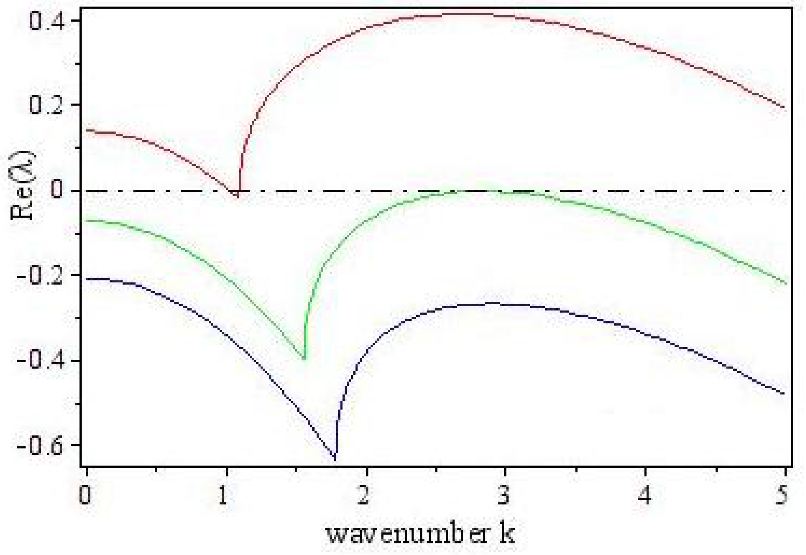
3.2. Turing Instability

In order to investigate the transition of the equilibrium state, we consider small space- and time-dependent perturbations for any solution of Equation (3):

(44)

where $\epsilon$, $\tau$ are small enough, $k$ is the wave number. Substituting Equation (44) into Equation (3), we linearize the system around $E_{*}$ and further obtain its characteristic equation:

(45)

where:

(46)

From Equation (45), the dispersion relation of Equation (3) is:

(47)

Turing instability requires that the stable interior equilibrium point is driven unstable by the local dynamics and diffusion of species. The conditions for the homogeneous state of Equation (2) to be stable is $t{r}_0=A+R<0$, ${\text{Δ}}_0=AR-BQ>0$. It is clear that $t{r}_k<t{r}_0$. Then the stability of the homogeneous state simultaneously changes the sign of ${\text{Δ}}_k$. From Equation (46), it easily finds that there is ${\text{Δ}}_k<0$ for ${{\kappa }_1}^2<k^2<{{\kappa }_2}^2$,where:

(48)

If ${{\kappa }_{1,2}}^2$ have positive values, we can obtain the range of instability for a local stable equilibrium, which is called as the Turing space. In order to show the Turing space, the dispersion relation is plotted corresponding to several values of the bifurcation parameter $m$ while in Figure 1 the other parameters are fixed as:

(49)

It should be stressed from Figure 1 that the available Turing modes are further reduced when the value of prey refuge $m$ is increasing. Nonetheless, it is interesting to notice that Equation (3) will occur the Turing instability when the value of $m$ less than $0.2512032$.

Figure 1. Variation of dispersion relation of Equation (3) around the interior equilibrium point. The red line corresponds to $m=0.08$, the green is $m=0.25$ and the blue is $m=0.35$.

Figure 1. Variation of dispersion relation of Equation (3) around the interior equilibrium point. The red line corresponds to $m=0.08$, the green is $m=0.25$ and the blue is $m=0.35$.

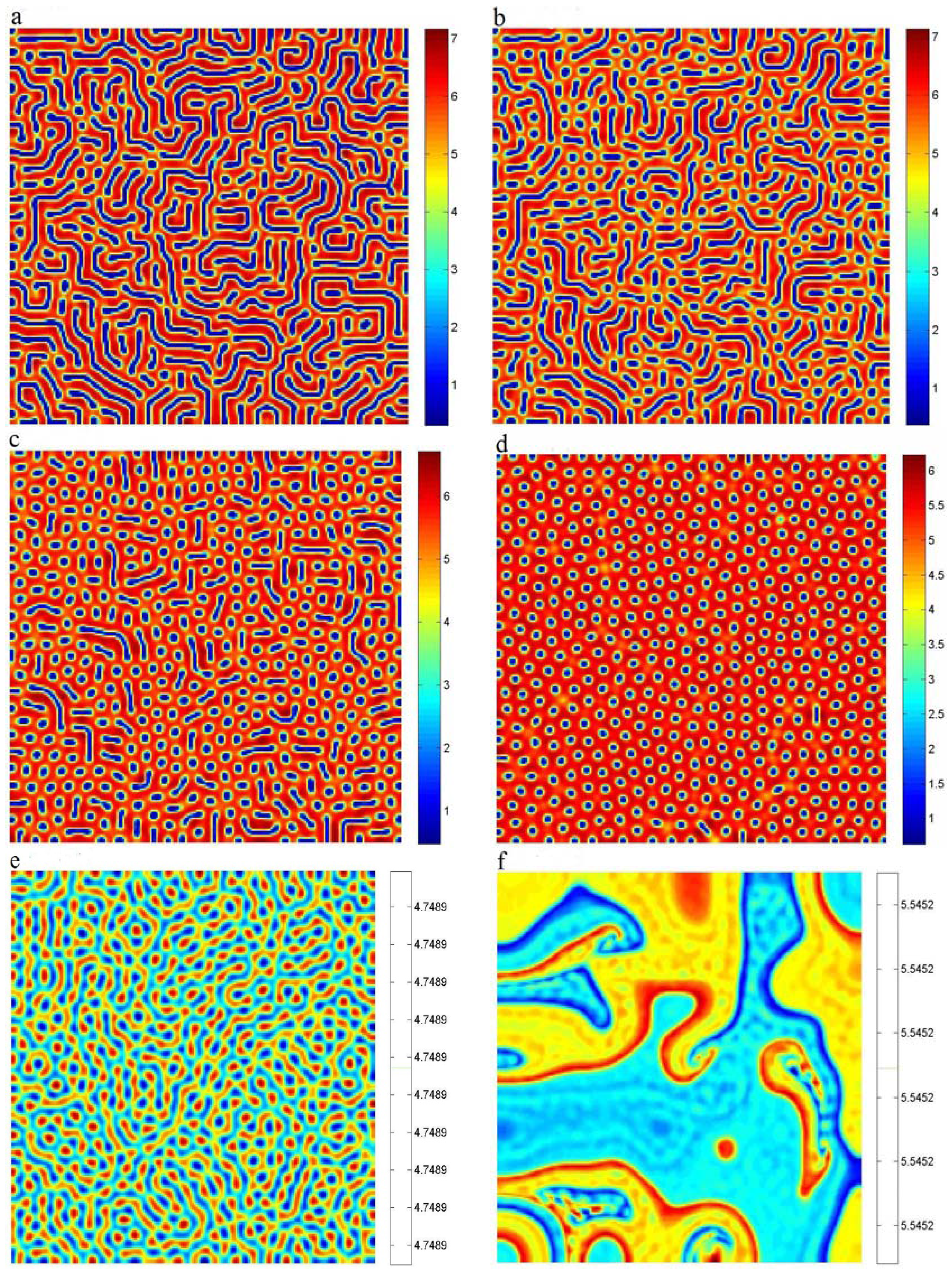
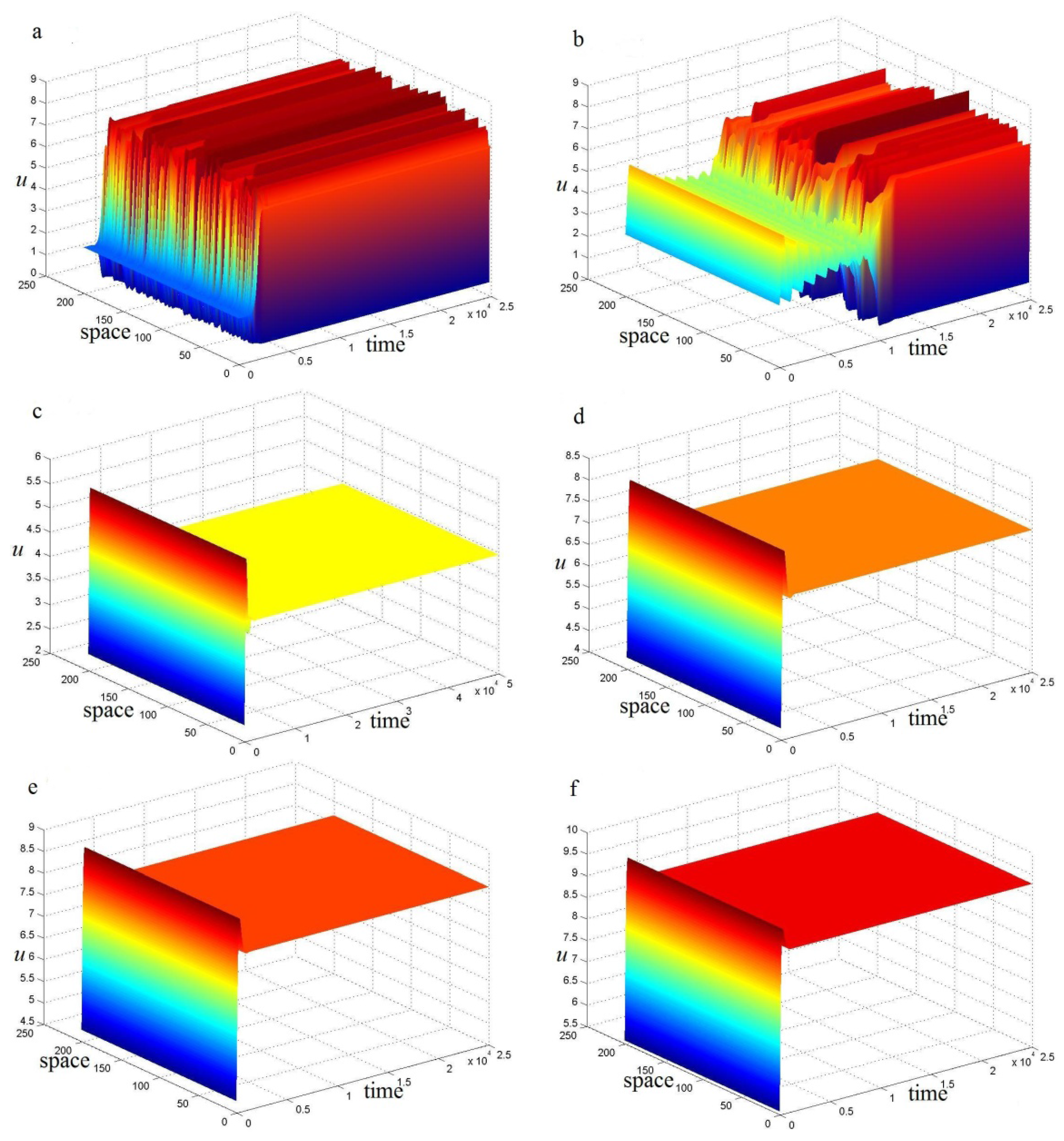
4. Turing Pattern Formation

To better investigate how the prey refuge affects the spatiotemporal dynamics of Equation (3), the spatial distribution diagrams are obtained as change of $m$. All numerical simulations are carried out in a discrete two-dimensional domain with $200\times 200$ lattice sites. The step between each lattice point is defined as $\omega =0.25$. The time evolution of Equation (3) is resorted to the forward Euler integration with a step $\upsilon =0.01$. The initial value of Equation (3) is placed in the stationary state $(u_{*},w_{*})$ and the perturbation for this value is $0.0005$ space units per time unit. As the initial perturbation propagates, Equation (3) under the condition of Turing instability evolves a steady state, which is stationary in time and oscillatory in space. Moreover, it should be stressed that the spatial patterns of predator and prey under the condition of Turing instability are always the same type, this is because that it is assumed that the carrying capacity of predator is proportional to the number of prey, and the steady state of predator is equal to this carrying capacity. Thus, only the spatial patterns of prey are shown.

It is interesting to note from Figure 2 that some snapshots have been taken of numerical simulations when the value of $m$ increases from $0$ to $0.35$. It should be pointed out that in these snapshots the enclosed color bars denote the range of the changing densities of prey, where higher values correspond to higher prey densities. Figure 1 clearly shows that Equation (3) leads to the Turing instability for $m<0.2512032$. The snapshots for $m=0$, $m=0.08$, $m=0.15$ and $m=0.22$ are chosen to report the spatial (oscillatory) and temporal (stationary) dynamics of Equation (3) around the interior equilibrium point, but the snapshots for $m=0.27$ and $m=0.35$ stand for the stable spatiotemporal behavior. By comparing the first four diagrams, it can be observed that the spatiotemporal dynamical behaviors of Equation (3) are very rich and complex. When the value of $m$ is $0$, the spatial distribution of prey is mainly some interconnected strips and nonuniform, which shows that the habits of prey are the main type of community survival, so it is easy to evade predator-capturing. When the values of $m$ are $0.08$ and $0.15$, the collective survival population expands gradually and the spatial distribution of prey tends to be uniform. When the value of $m$ is $0.22$, the spatial distribution of prey is almost uniform and the prey can survive in any space. On the other hand, from Figure 2 the maximum values on color bars exhibit decreasing states as the effect of prey refuge is strengthened. Inversely, the interior equilibrium density value of prey will increase as the increase of m. In order to relieve the crowed space, the competitive pressure between individuals of prey is intensified. From the biological point of view, the effect of prey refuge may be to help prey relieve the pressure of predation during diffusion. Thus, the patches of high density prey diffuse into the low. Finally, the distributions of prey tend to be uniform as the effect of prey refuge increases. However, when the value of $m$ is more than $0.2512032$, the prey and the predator will be involved into a stable state, so the prey can live in any space, which can be shown in behind two diagrams of Figure 2. These results show that the prey refuge not only promotes an increase in the number of prey, but also is conducive to their living space extension.

For further analysis of the effect of prey refuge on the dynamical behavior of one population, the spatiotemporal evolutions of prey have been obtained at $x=100$, which correspond to Figure 2. It should be stressed from Figure 3 that these results are consistent with Figure 2, which show the accuracy and effectiveness of numerical simulations. Moreover, the comparison of the first four diagrams in Figure 3 suggests that when the value of $m$ gradually increases and is close to $0.2512032$, oscillations in space diminish gradually. These results show that a suitable prey refuge has a positive effect on predator-prey interactions. It is easy to see that if the effect of prey refuge is strengthened in living surroundings, predation risk is relatively reduced in the habitat and consequently the density of prey is bound to increase. And the densities of predator and prey will obtain the new balance.

Based on the above analysis, it can be seen that a suitable prey refuge can enhance the specie biomass level and promote the uniformness of the population distribution, which agree with some results of the real world. Furthermore, it is interesting to point out that the lower value of prey refuge can come into rich spatiotemporal dynamics. Moreover, the use of mathematical model with a prey refuge and diffusion is considered to explore some biological problems, and the numerical simulation can provide an approximation of the real biological behaviors. Hence, these results can promote the study of ecological patterns.

Figure 2. Spatial distributions of prey obtained with Equation (3) for (a) $m=0$, (b) $m=0.08$, (c) $m=0.15$, (d) $m=0.22$, (e) $m=0.27$, (f) $m=0.35$. Other parameters are fixed as Equation (49).

Figure 2. Spatial distributions of prey obtained with Equation (3) for (a) $m=0$, (b) $m=0.08$, (c) $m=0.15$, (d) $m=0.22$, (e) $m=0.27$, (f) $m=0.35$. Other parameters are fixed as Equation (49).

Figure 3. The spatiotemporal evolutions of prey obtained with Equation (3) at x = 100. (a) $m=0$, (b) $m=0.08$, (c) $m=0.15$, (d) $m=0.22$, (e) $m=0.27$, (f) $m=0.35$. Other parameters are fixed as Equation (49).

Figure 3. The spatiotemporal evolutions of prey obtained with Equation (3) at x = 100. (a) $m=0$, (b) $m=0.08$, (c) $m=0.15$, (d) $m=0.22$, (e) $m=0.27$, (f) $m=0.35$. Other parameters are fixed as Equation (49).

5. Conclusions

In this paper, a diffusive predator-prey system with Holling type III scheme has been studied analytically and numerically. Mathematical theoretical works have considered the existence of global solutions and the stability of equilibrium points and population permanence. On the basis of these results, we obtain the threshold expressions of some critical parameters which in turn provide a theoretical basis for the numerical simulation. Numerical simulations indicate that the prey refuge has a strong and positive effect on the spatiotemporal dynamics according to the spatial patterns and spatiotemporal evolution of prey. Furthermore, it should be stressed that the spatial pattern diagrams show that the prey refuge has a profound effect on predator-prey interactions. Using the spatiotemporal evolution of prey, the spatial distribution of prey and the accuracy effectiveness of numerical simulation can be further confirmed. All these results are expected to be of significance in the exploration of the entropy theory of bioinformatics.

References

1. Baek, H. A food chain system with Holling type IV functional response and impulsive perturbations. Comput. Math. Appl. 2010, 60, 1152–1163. [Google Scholar] [CrossRef]
2. Zhao, M.; Lv, S.J. Chaos in a three-species food chain model with a Beddington-DeAngelis functional response. Chaos Soliton. Fract. 2009, 40, 2305–2316. [Google Scholar] [CrossRef]
3. González-Olivares, E.; González-Yañez, B.; Lorca, J.M.; Rojas-Palma, A.; Flores, J.D. Consequences of double Allee effect on the number of limit cycles in a predator–prey model. Comput. Math. Appl. 2011, 62, 3449–3463. [Google Scholar] [CrossRef]
4. Yu, H.G.; Zhong, S.M.; Agarwal, R.P.; Xiong, L.L. Species permanence and dynamical behavior analysis of an impulsively controlled ecological system with distributed time delay. Comput. Math. Appl. 2010, 59, 382–3835. [Google Scholar] [CrossRef]
5. Zhao, M.; Wang, X.T.; Yu, H.G.; Zhu, J. Dynamics of an ecological model with impulsive control strategy and distributed time delay. Math. Comput. Simul. 2012, 82, 1432–1444. [Google Scholar] [CrossRef]
6. Chen, S.S.; Shi, J.P.; Wei, J.J. A note on Hopf bifurcations in a delayed diffusive Lotka-Volterra predator-prey system. Comput. Math. Appl. 2011, 62, 2240–2245. [Google Scholar] [CrossRef]
7. Zhao, M.; Zhang, L. Permanence and chaos in a host-parasitoid model with prolonged diapause for the host. Commun. Nonlinear Sci. Numer. Simul. 2009, 14, 4197–4203. [Google Scholar] [CrossRef]
8. Yu, H.; Zhao, M. Seasonally perturbed prey-predator ecological system with the Beddington-DeAnglis functional response. Discrete Dyn. Nat. Soc. 2012, 2012, 150359. [Google Scholar] [CrossRef]
9. Liu, Z.J.; Zhong, S.M. Permanence and extinction analysis for a delayed periodic predator-prey system with Holling type II response function and diffusion. Appl. Math. Comput. 2010, 216, 3002–3015. [Google Scholar] [CrossRef]
10. Huo, H.F.; Li, W.T. Periodic solutions of delayed Leslie-Gower predator-prey models. Appl. Math. Comput. 2004, 155, 591–605. [Google Scholar] [CrossRef]
11. Yuan, S.L.; Song, Y.L. Bifurcation and stability analysis for a delayed Leslie-Gower predator-prey system. IMA J. Appl. Math. 2009, 74, 574–603. [Google Scholar] [CrossRef]
12. Leslie, P.H. Some further notes on the use of matrices in population mathematics. Biometrika 1948, 35, 213–245. [Google Scholar] [CrossRef]
13. Leslie, P.H.; Gower, J.C. The properties of a stochastic model for the predator–prey type of interaction between two species. Biometrika 1960, 47, 219–234. [Google Scholar] [CrossRef]
14. Aziz-Alaoui, M.A.; Okiye, M.D. Boundedness and global stability for a predator-prey model with modified Leslie-Gower and Holling type II schemes. Appl. Math. Lett. 2003, 16, 1069–1075. [Google Scholar] [CrossRef]
15. Kox, M.; Sayler, G.S.; Schultz, T.W. Complex dynamics in a model microbial system. Bull. Math. Biol. 1992, 54, 619–648. [Google Scholar]
16. Apreutesei, N.; Dimitriu, G. On a prey-predator reaction-diffusion system with a Holling type III functional response. J. Comput. Appl. Math. 2010, 235, 366–379. [Google Scholar] [CrossRef]
17. Liu, Z.; Zhong, S.; Liu, X. Permanence and periodic solutions for an impulsive reaction-diffusion food-chain system with Holling type III functional response. J. Franklin Inst. 2011, 348, 277–299. [Google Scholar] [CrossRef]
18. Schenk, D.; Bacher, S. Functional response of a generalist insect predator to one of its prey species in the field. J. Anim. Ecol. 2002, 71, 524–531. [Google Scholar] [CrossRef]
19. Sugie, J.; Miyamoto, K.; Morino, K. Absence of limit cycles of a predator-prey system a sigmoid functional response. Appl. Math. Lett. 1996, 9, 85–90. [Google Scholar] [CrossRef]
20. Lamontagne, Y.; Coutu, C.; Rousseau, C. Bifurcation analysis of a predator–prey system with generalized Holling type III functional response. J. Dyn. Diff. Equ. 2008, 20, 535–571. [Google Scholar] [CrossRef]
21. Hochberg, M.E.; Hold, R.D. Refuge evolution and the population dynamics of coupled host-parasitoid association. Evol. Ecol. 1995, 9, 633–661. [Google Scholar] [CrossRef]
22. Ma, Z.H.; Li, W.L.; Zhao, Y.; Wang, W.L.; Zhang, H.; Li, Z.Z. Effects of prey refuges on a predator-prey model with a class of functional responses: The role of refuges. Math. Biosci. 2009, 218, 73–79. [Google Scholar] [CrossRef] [PubMed]
23. Guan, X.N.; Wang, W.M.; Cai, Y.L. Spatiotemporal dynamics of a Leslie-Gower predator-prey model incorporating a prey refuge. Nonlinear Anal. Real World Appl. 2011, 12, 2385–2395. [Google Scholar] [CrossRef]
24. Huang, Y.J.; Chen, F.D.; Zhong, L. Stability analysis of a prey-predator model with Holling type III response function incorporating a prey refuge. Appl. Math. Comput. 2006, 182, 672–683. [Google Scholar] [CrossRef]
25. Gonzalez-Olivares, E.; Ramos-Jiliberto, R. Dynamic of prey refuges in a simple model system: More prey, fewer predators and enhanced stability. Ecol. Modell. 2003, 166, 135–146. [Google Scholar] [CrossRef]
26. Jia, Y.F.; Xu, H.K.; Agarwal, R.P. Existence of positive solutions for a prey-predator model with refuge and diffusion. Appl. Math. Comput. 2011, 217, 8264–8276. [Google Scholar]
27. Camara, B.I. Waves analysis and spatiotemporal pattern formation of an ecosystem model. Nonlinear Anal. Real World Appl. 2011, 12, 2511–2528. [Google Scholar] [CrossRef]
28. Turing, A.M. The chemical basis of morphogenesis. Philos. Trans. R. Soc. Lond B: Biol. Sci. 1952, 237, 37–72. [Google Scholar] [CrossRef]
29. Zhu, L.M.; Wang, A.L.; Liu, Y.J.; Wang, B. Stationary patterns of a predator-prey model with spatial effect. Appl. Math. Comput. 2010, 216, 3620–3626. [Google Scholar] [CrossRef]
30. Aly, S.; Kima, I.; Sheen, D. Turing instability for a ratio-dependent predator-prey model with diffusion. Appl. Math. Comput. 2011, 217, 7265–7281. [Google Scholar] [CrossRef]
31. Banerjee, M.; Petrovskii, S. Self-organised spatial patterns and chaos in a ratio-dependent predator-prey system. Theor. Ecol. 2011, 4, 37–53. [Google Scholar] [CrossRef]
32. Tian, Y.L.; Weng, P.X. Stability analysis of diffusive predator-prey model with modified Leslie-Gower and Holling type III schemes. Appl. Math. Comput. 2011, 218, 3733–3745. [Google Scholar] [CrossRef]