Maximum Entropy Distributions Describing Critical Currents in Superconductors

Abstract

Maximum entropy inference can be used to find equations for the critical currents (J_c) in a type II superconductor as a function of temperature, applied magnetic field, and angle of the applied field, θ or ϕ. This approach provides an understanding of how the macroscopic critical currents arise from averaging over different sources of vortex pinning. The dependence of critical currents on temperature and magnetic field can be derived with logarithmic constraints and accord with expressions which have been widely used with empirical justification since the first development of technical superconductors. In this paper we provide a physical interpretation of the constraints leading to the distributions for J_c(T) and J_c(B), and discuss the implications for experimental data analysis. We expand the maximum entropy analysis of angular J_c data to encompass samples which have correlated defects at arbitrary angles to the crystal axes giving both symmetric and asymmetric peaks and samples which show vortex channeling behavior. The distributions for angular data are derived using combinations of first, second or fourth order constraints on cot θ or cot ϕ. We discuss why these distributions apply whether or not correlated defects are aligned with the crystal axes and thereby provide a unified description of critical currents in superconductors. For J//B we discuss what the maximum entropy equations imply about the vortex geometry.

1. Introduction

The most important property of a superconductor from a practical viewpoint is the critical electrical current density (J_c, measured in Am⁻², or for thin films the sheet current, I_c in A/cm is often recorded) under the operating conditions of temperature (T) and applied magnetic field (B). This is the current above which power dissipation increases rapidly and the material transitions to a non-superconducting state and it determines the useful current-carrying capacity of a superconducting wire or film. A better understanding of critical currents is therefore of interest both practically and from a fundamental physics viewpoint. Remarkably the phenomenology of critical currents remains poorly understood. There are many models of critical currents [1,2,3,4] but these often fail to adequately reproduce basic features of experiments. In this paper we show how a maximum entropy approach results in a unified framework for understanding the phenomenology of critical currents in superconductors and provides insight that would be impossible to attain when working from deterministic models.

In reality superconductors do not transition abruptly from the superconducting to the non-superconducting state. The electric field–current density (E–J) relationship is usually a power law, $E/E_0={(J/J_c)}^n$ with n ~ 10–100 for different samples and conditions [5]. The critical current is therefore a parameter in a constitutive equation and is defined as the DC current carried when the sample satisfies a particular electric field criterion, usually E₀ = 10⁻⁴ Vm⁻¹, parallel to the transport current direction; this is the value most often recorded in experiments.

From a physics perspective we wish to connect critical currents with magnetic flux vortex behavior [1,2,3,4]. Flux vortices are the quantized magnetic fluxons which penetrate type II superconductors subjected to an applied magnetic field. They are whirlpools of supercurrents surrounding a non-superconducting core and can be modeled as elastic strings threading through the superconductor in global alignment with the macroscopic field direction. Vortices will preferentially align themselves with pre-existing non-superconducting regions of the material (e.g., material defects) so as to lower the total free energy of the system. This preferential alignment with a non-superconducting region is termed “pinning”. It requires a force of order ΔU/2ξ to dislodge a vortex from a pinned position, where ΔU is the difference in condensation energy between the pinned and free vortex and 2ξ is the lateral dimension of the vortex core. When vortices move, energy is dissipated in the sample, ultimately leading to a loss of superconductivity. For high critical currents to be achieved, vortices must remain immobile or “pinned” in the material.

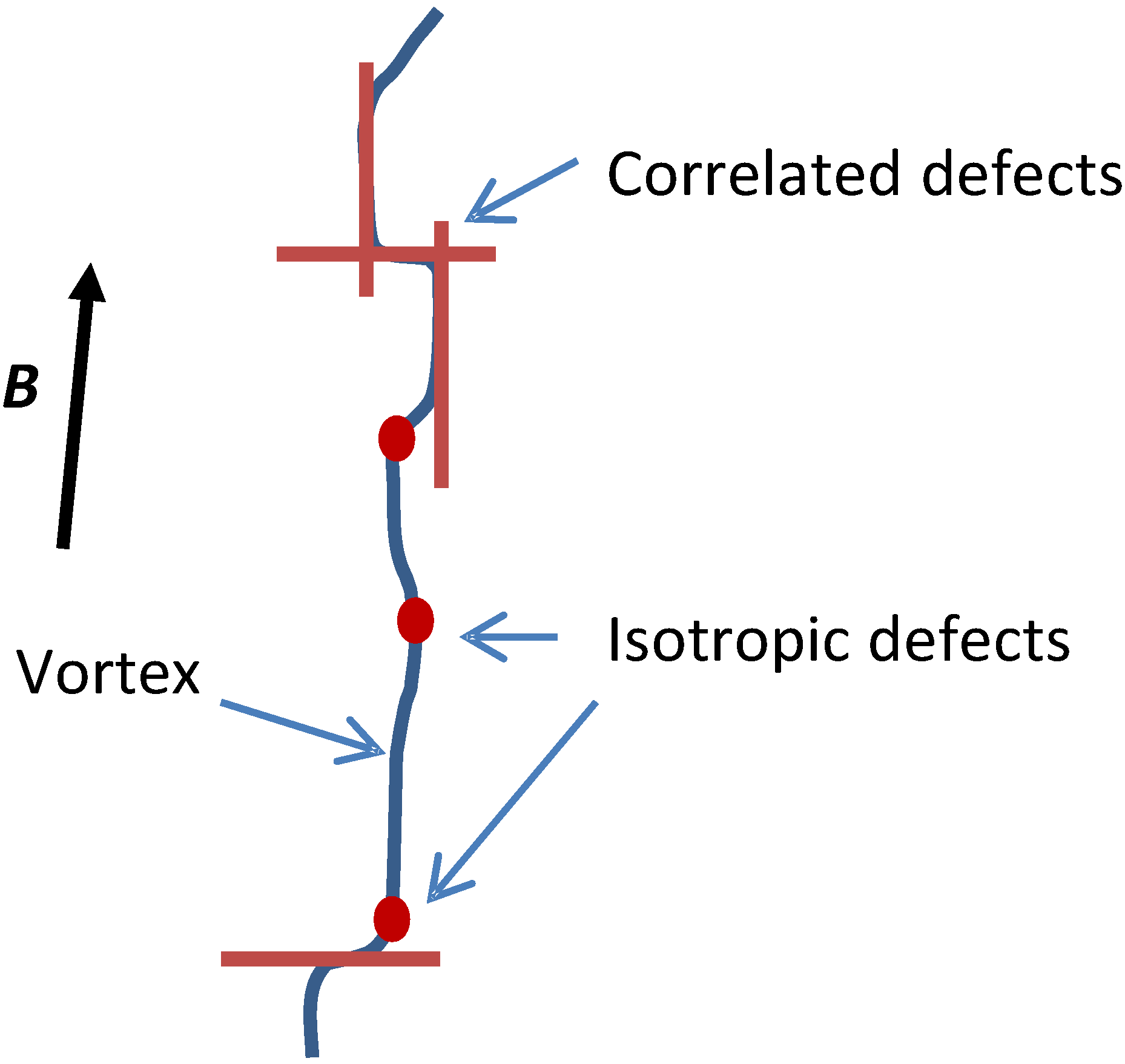
Most models of J_c begin with a definition, first proposed by P. W. Anderson [6], that equates the flux pinning force per unit volume (F_p) in the sample with the Lorentz force experienced by the vortex lattice under the influence of an electrical current, ${\overrightarrow{F}}_p={\overrightarrow{J}}_c\times \overrightarrow{B}$. The challenge then is to model ${\overrightarrow{F}}_p$ in terms of the total available pinning in the sample and the interaction between vortices themselves. The total available pinning, often referred to as the “pinning landscape”, is usually modeled through an enumeration of “defects” or “pinning centers”. The density of defects is labeled n_p and the flux pinning force per unit length of vortex, created by a defect or defects, labeled f_p. The defects may be of many different scales, shapes, and chemistry. Some are point defects, and some are extended and correlated with the crystal axes. Grain boundaries will act as pinning centers, and surfaces, pores and interfaces can also provide a pinning force. Some defects are second phase material intentionally introduced and some are intrinsic features of a crystal structure. We show a schematic diagram of a vortex in Figure 1 which is pinned by both isotropic defects, e.g. non-superconducting nanoparticle inclusions, and correlated defects, e.g. stacking faults and twin plane boundaries.

Models of ${\overrightarrow{F}}_p$ must then consider vortices interacting with the pinning landscape and each other. Without pinning, vortices preferentially arrange themselves into a triangular lattice due to the interactions between vortices. The effects of vortex-vortex interactions may be modeled through defining elastic constants of the vortex lattice, and such phenomena as shear of the vortex lattice can be considered. Flux pinning is also affected by thermal excitations and local variations in electromagnetic fields.

Unfortunately, no deterministic model of the pinning landscape provides a unified explanation of the behavior of J_c with temperature and field, few show any predictive power, and because the Lorentz force definition fails when $\overrightarrow{J}//\overrightarrow{B}$, none describe the behavior under all conditions. The outstanding issue is the “pinning summation problem”. That is, there is no reliable methodology to sum the effects of all the defects distributed throughout a material in order to find ${\overrightarrow{F}}_p$.

We have shown previously [7,8,9,10] how by adopting a maximum entropy approach we can model J_c while avoiding the need to construct a model of ${\overrightarrow{F}}_p$. Although we do not solve the pinning summation problem in the sense of making direct predictions of the magnitude of J_c we do gain insight into how nature averages over all defects and interactions and what information is available from any experiment. In this paper we extend our analysis to include a greater range of critical current data. In Section 2 we briefly explain how we apply the maximum entropy formalism. In Section 3 we demonstrate how particular simple choices of constraints provide distributions which describe essentially all reported results for critical currents as a function of temperature, magnetic field, and field angle. In particular we show that previous expressions for J_c(θ) which apply to defects correlated with the crystal axes also apply for combinations of defects not aligned to the crystal axes. We also show for the first time that angular data related to vortex channeling can be described by including 4^th order constraints on cotθ. In Section 4 we offer a physical interpretation of the field and temperature constraints. The geometric shape of vortices particularly for J//B implied by the angular constraints is discussed.

Figure 1. Schematic diagram of a pinned magnetic vortex. Macroscopically the vortex follows the applied field direction B; microscopically it is distorted by the particular pinning centers with which it interacts and by the effect of the local electromagnetic field.

Figure 1. Schematic diagram of a pinned magnetic vortex. Macroscopically the vortex follows the applied field direction B; microscopically it is distorted by the particular pinning centers with which it interacts and by the effect of the local electromagnetic field.

2. Maximum Entropy Method

Deterministic models of critical currents as described above pose the question, “What force is required to move a pinned vortex?” and J_c is defined at the point of force balance between motive force and pinning force. In the maximum entropy approach we ask instead, “What is the probability a vortex is pinned?” We therefore propose the ansatz J_c(υ) dυ = J₀ p(υ) dυ where p(υ) is the normalized probability a vortex is pinned over the domain of υ. J₀ is a constant which does not depend on υ and which we determine from experiment. This is not the only possible physical interpretation of p(υ)dυ. We could equally regard it as the probability a quasi-particle in the sample contributes to the current transport. This is equivalent to directly considering it as the probability for how an “element” δJ_c of critical current is distributed across the domain. In this paper we choose to relate our equations to flux vortex behavior as this is the usual conceptual framework in which to understand critical currents.

To assign the probabilities p(υ) we apply the Principle of Maximum Entropy [11,12]. We choose the distribution which maximizes the Shannon information entropy, S_I = −∫p(υ)lnp(υ)dυ subject to constraints of the form < g_r(υ) ≥ ∫p(υ)g_r(υ)dυ; r = 1, 2, .., m.. The general solution is $p(\upsilon )=\exp (-{\lambda }_0-{\lambda }_1{g}_1(\upsilon )-{\lambda }_2{g}_2(\upsilon )-\dots -{\lambda }_m{g}_m(\upsilon ))$, where λ_ι are Lagrange multipliers. This ensures we obtain the least biased distribution among all possible choices that satisfies the given constraints. If we include all the constraints operating in the physical system, then the distribution obtained through maximizing the information entropy is overwhelmingly the most likely to be observed experimentally. We treat the procedure as one of trial and error in which we assume simple constraints and then proceed to fit the derived distribution to experimental data. If this distribution accurately describes the data then we have found a valid model. If the distribution does not adequately fit our data then either additional constraints exist or we have used the wrong constraints. As a consequence, which has been emphasized by Jaynes [13], even a failure of the procedure is valuable – a failure means we should reassess our constraints and the discrepancy between data and model can help us to uncover new physics.

3. Results and Discussion

The behavior we are interested in modeling is how the critical current density (J_c) changes with temperature (T), magnitude of an applied magnetic field (B), and the direction of the applied field (θ,ϕ). We will look at each of these in turn.

3.1. Temperature Dependence of J_c

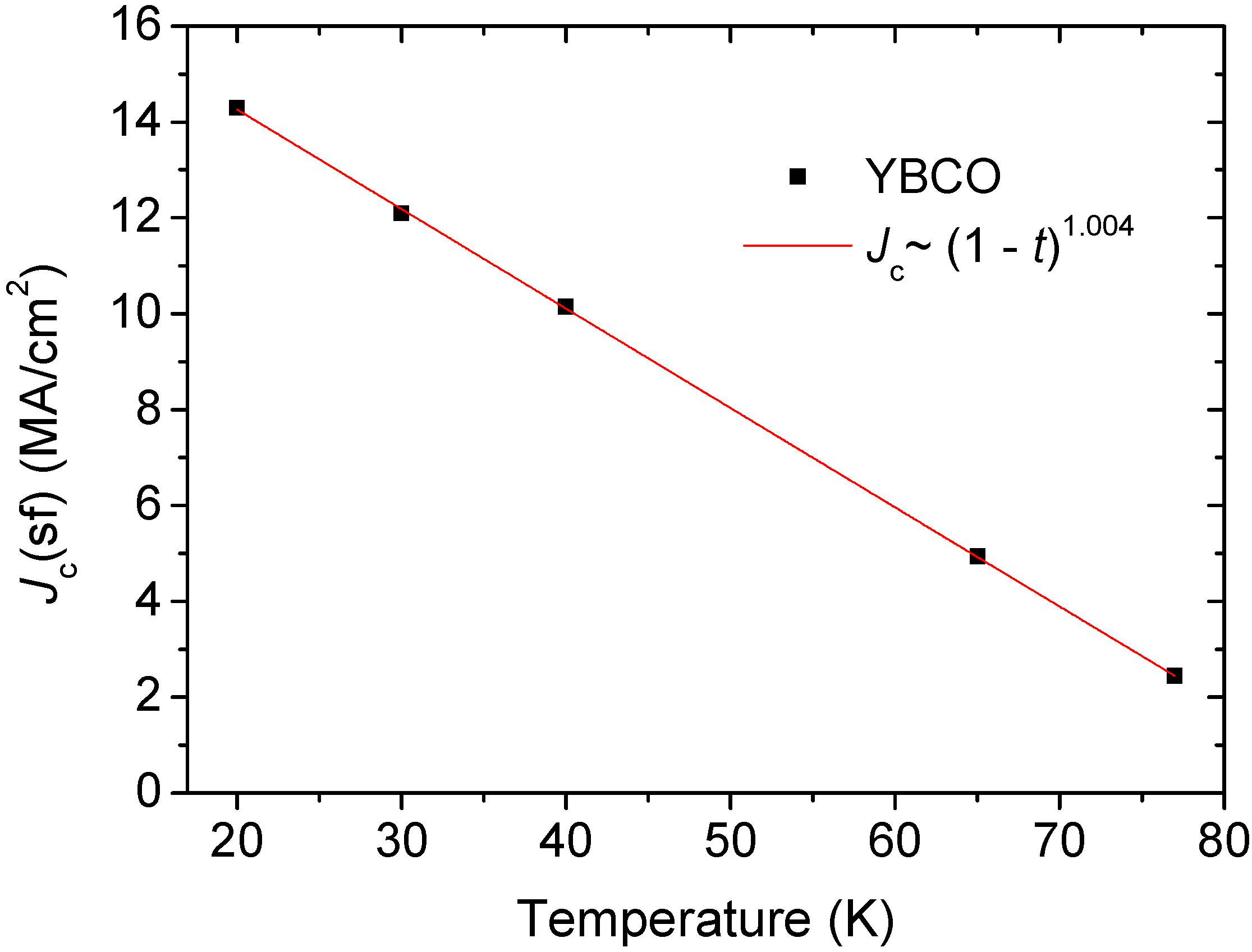
We first examine the temperature dependence, which is of particular relevance for high temperature superconductor (HTS) samples which operate over a wide temperature range. Critical currents only exist between T = 0, and T = T_irr, where T_irr is an irreversibility temperature beyond which vortices cannot be pinned. We can normalize $t=T/T_{irr}$ and our data falls on the domain $0<t<1$. For temperature dependent data in HTS the form most often employed in experimental analysis is $J_c(t)~{(1-t)}^{\delta }$ [14,15]. In Figure 2 we show a measurement of J_c(T) which follows this form with δ = 1. Typically for YBCO films prepared in our laboratory we obtain data with δ ~ 1–2 [16]. There has been no convincing explanation to date why this functional form is persistently observed for samples with such a variety of microstructures. We can recognize this form as a power law which comes from a constraint of the expectation value, $<\ln (1-t)>=\ln (1-g)$ [12]. If we maximize the Shannon information entropy using this constraint we obtain using our ansatz for J_c:

$$J_c(t)=\frac{J_0}{\ln (1/(1-g))}{(1-t)}^{1/\ln (1/(1-g))-1}$$

(1)

Some data for high temperature superconductor (HTS) samples follows a mixture form [14,15], $J_c(t)~w_1{J}_1+w_2{J}_2$. From the maximum entropy point of view this is not surprising. It suggests the sample has physical populations of defects which are sufficiently different in their overall properties that they create distinct constraints which can be resolved in the macroscopic experiment. It is therefore a natural extension of the model. For example, at low temperature we may have an effective physical population of defects which is statistically distinct from the physical population effective at high temperatures. In low temperature superconductors (LTS) the form $J_c~{(1-t^2)}^{\delta }$ has sometimes been used to fit data [1]. At temperatures close to T_c, and for the limited range of LTS temperature data, this form can be difficult to distinguish from Equation (1). We therefore consider we have a well validated maximum entropy expression for J_c(T). The physical meaning of the constraint is discussed in Section 4.

Figure 2. J_c(T) for a metal-organic deposited YBCO thin film, 1 μm thickness.

Figure 2. J_c(T) for a metal-organic deposited YBCO thin film, 1 μm thickness.

3.2. Magnetic Field Dependence of J_c

There are three possible sources of field in a measurement of J_c: external sources, B_ex; transport current self-field (the field generated by the transport current itself), B_sf; and equilibrium magnetization currents producing fields of the order B_c1. The maximum field for the measurement is the irreversibility field, B_irr; the field at which it is no longer possible for the sample to sustain a measurable critical current, i.e. J_c = 0. External fields are usually significantly larger than B_c1 and B_sf, so that experimental data falls in the range B_c1 << B_sf << B_ext < B_irr. If we ignore the smaller field sources for the moment, then $B\approx B_{ext}$ and $b=B/B_{irr}$ and we have $J_c(b)$ on the domain $0<b<1$. Rather than a direct analysis of $J_c(b)$ it is common to plot the pinning force, $F_p=J_{c}B$, against B or b, forming a normalized plot of flux pinning force versus (normalized) field for $\overrightarrow{B}\perp \overrightarrow{J}$. It has been known for the past 40 years that such a plot takes the form $F_p~b^m{(1-b)}^n$ [1,2,17,18]. This is true of both LTS and HTS samples. In the words of Campbell and Evetts ([2] p.159), “A frequent and striking feature of these curves is that over a wide range of microstructures, field and temperatures they have the same shape”. This was written before it was observed that the high temperature superconductors and MgB₂ also obey this form [19]. Various explanations have been offered for this, but without consensus. The same shape implies that data over multiple conditions can be scaled to a common curve, a useful property for constructing empirical models used in engineering of devices [20].

We can notice that this form is a beta distribution; the multiplication by b or B, doesn’t alter this form. The beta distribution can be derived from maximum entropy using logarithmic constraints, $<\ln b>$ and $<\ln (1-b)>$ [12]. For the field dependence we thus have the equation:

$$J_c(b)=\frac{J_0}{Beta(\alpha ,\beta )}{b}^{\alpha -1}{(1-b)}^{\beta -1}$$

(2)

where $<\ln b>=\mathrm{\Psi }(\alpha )-\mathrm{\Psi }(\alpha +\beta )$, and $<\ln (1-b)>=\mathrm{\Psi }(\beta )-\mathrm{\Psi }(\alpha +\beta )$ where Ψ is the digamma function.

An example of the ability to scale data under different conditions to a common curve is shown in Figure 3 for a Bi-2223 tape sample, manufactured by AMSC (Devens, MA, USA). Here we have scaled data for different field directions to show the common form. The irreversibility fields used in the scaling range from B_irr= 1.73 T at 0° (field perpendicular to the plane of the sample) to B_irr= 11.1 T at 90° (field parallel to the plane of the tape). The Bi-2223 material is highly anisotropic therefore the accommodation of vortices to the pinning landscape must be very different at the different angles. The scaling to a common curve emphasizes the statistical nature of the macroscopic response. We discuss the implications for analyzing the sources of pinning in more detail in Section 4.

One circumstance which is known to occur [1] in which Equation (2) fails in the form $F_p~b^m{(1-b)}^n$, is when the data is better fitted with two or more components, i.e. weighted contributions,$F_p~w_1{F}_1+w_2{F}_2$. Again this is not surprising, suggesting the sample has physical populations of defects which are sufficiently different in their overall properties that the outcome is a mixture distribution. In [10] we give an example where J_c(B) data with a secondary maximum at intermediate fields (a so-called “peak effect”) can be described using this form.

A more accurate fitting to the model should also take into account the smaller field sources which we have ignored, so that $b\approx B/B_{irr}$ is a measure of the field in the sample. For example, we could rescale the B axis to account for self-fields. As this mainly affects the low field region it probably has little practical effect on the fitting parameters obtained.

The maximum entropy distribution for field dependence is thus well established in the superconductivity literature. We give a physical interpretation of the constraints in Section 4, and we also discuss what the maximum entropy viewpoint implies for the interpretation of experimental results.

Figure 3. Flux pinning force as a function of applied field for a Bi-2223 wire sample measured at 77 K. The data for 4 different field angles, θ = 0 (perpendicular field), 30°, 60° and 90° (parallel field) are scaled to lie on a common curve. The Beta distribution parameters used to fit the common curve are, α=1.8, β = 9.6.

Figure 3. Flux pinning force as a function of applied field for a Bi-2223 wire sample measured at 77 K. The data for 4 different field angles, θ = 0 (perpendicular field), 30°, 60° and 90° (parallel field) are scaled to lie on a common curve. The Beta distribution parameters used to fit the common curve are, α=1.8, β = 9.6.

3.3. Out-of-Plane Field Angular Dependence of J_c Under Maximum Lorentz Force

For a planar sample lying in the xy plane, with current direction $\overrightarrow{J}=J_x$, θ is the angle of the magnetic field in the yz plane, (i.e. $B\perp \widehat{x}$, θ = 90° for field direction parallel to $\widehat{y}$) and ϕ is the angle in the xy plane (i.e. $B\perp \widehat{z}$, ϕ = 90°for field direction parallel to $\widehat{x}$). We consider first the case where the magnetic field is kept perpendicular to the current direction (ϕ = 0, maximum Lorentz force configuration). We maximize $S=-{\displaystyle {\int }_0^{\pi }f(\theta )\ln (f(\theta ))d\theta }$ where $J_c(\theta )=J_{0}f(\theta )$, with ${\displaystyle \int f(\theta )d\theta =1}$, subject to chosen constraints <g(θ)>. If there are no constraints we obtain a uniform distribution:

$$J_c(\theta )=J_0/\pi$$

(3a)

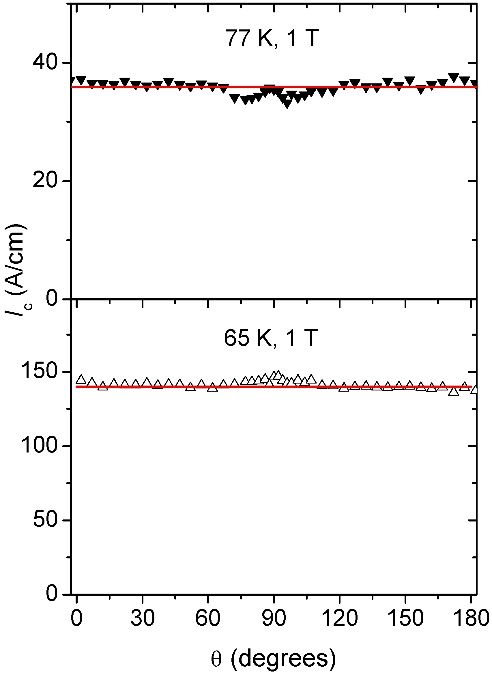
For fully isotropic superconductors, for example, a round wire of the LTS conductor Nb-Ti, such an angular dependence is a trivial result. Of interest is whether this result has wider applicability. In Figure 4 we show J_c(θ) of a thin film HTS YBCO sample prepared by metal organic deposition [16]. To a good approximation we have a uniform distribution of critical current. This is a surprising result because the sample has many defects and pinning structures which are aligned with the crystal axes. Particularly the sample has stacking faults which are aligned with the film surface (90° direction)—normally these are correlated with the observation of strong peaks in J_c(θ) [21]. The sample also has grain boundaries, twin planes and twin plane intersections aligned normal to the film surface (0° direction) which are often correlated with the observation of J_c(θ) maxima. Even an intrinsically isotropic low temperature superconductor film usually has a peak in the direction parallel to the surface due to surface pinning as shown in the next section. In anisotropic high temperature superconductors the vortices themselves are dimensionally anisotropic due to the electronic mass anisotropy. Hence the local pinning forces are often presumed to always be anisotropic with θ and in spite of this, here we observe an almost isotropic response of the critical current.

Figure 4. Isotropic J_c(θ) observed in an anisotropic high temperature superconductor YBCO, (a) 77 K, (b) 65 K, data (▼, Δ), fit ($▬$).

Figure 4. Isotropic J_c(θ) observed in an anisotropic high temperature superconductor YBCO, (a) 77 K, (b) 65 K, data (▼, Δ), fit ($▬$).

In the experiments of Figure 4 the many factors which result in a vortex being pinned or not have averaged, such that there is no dependence on the angle of the applied field. This is a striking example of the loss of information on the microscopic state when making a macroscopic measurement. That is to say, the configurations of the pinned vortices must be quite different across all angles but this information is lost to the experimentalist. No deterministic model of J_c starting from a model of F_p which included anisotropic pinning structures would ever be likely to predict an angle independent J_c. The common assumption is that anisotropic structures must produce an anisotropic J_c [22], but here this is demonstrated to be false.

A more detailed analysis of when peaks are observed in these samples depending on the relative density of correlated defects is given in [16]. The point we are making here is that Equation 3a, is an important and valid maximum entropy distribution for describing J_c(θ). It is also highlights the necessity of an epistemic model for critical currents in analyzing data.

It is more usual when measuring thin film superconductors to observe peaks in J_c(θ) due to vortices’ interactions with pinning structures correlated with the crystal axes. For each pinned vortex i the vortex must be stationary over total pinned lengths y_i and z_i. The macroscopic angle at which the vortex is pinned satisfies $z_i/y_i=\cot ({\theta }_i)$. Rather than the summation of pinned vortex segments creating a mean angle $\overline{\theta }$ which is the relevant information, we consider the possibility it is the mean $<z/y>=<\cot \theta >$ which is relevant. Similarly, if a variance is constrained by the pinning landscape it is $<{((z/y)-<z/y>)}^2>$. (In our discussions we could equally use $<y/z>=<\tan \theta >$ etc, as the constraints for our derivation of the distributions. The choice of using z/y as the variable is to maintain consistency with the derivation in our earlier papers, particularly [8]. The original choice of z/y was made so that <z/y> = 0 positions the peak of the distribution at θ = 90° which is the common occurrence in HTS samples.)

This implies the most uniform distribution to describe correlated pinning is the improper distribution of a uniform p(z/y) on the domain $-\infty <0<\infty$. We can imagine this distribution as describing the pinning arising from an infinite square lattice of correlated pins in the y-z plane, in which any value of z/y is equally likely.

With constraints on the mean <z/y>, and variance <((z/y) − <z/y>)²>, it is well known that maximization of the information entropy gives a Gaussian distribution in z/y. By a simple transformation of random variables to the θ variable, $f_{\mathrm{\Theta }}(\theta )=f_{Z/Y}(h(\theta ))\left|dh(\theta )/d\theta \right|$, with $h=\cot \theta$, we obtain:

$$J_{\text{c}}(\theta )=\frac{J_0}{\sqrt{2\pi }\sigma {\sin }^2\theta }\exp \left(-\frac{1}{2{\sigma }^2{\tan }^2\theta }\right)$$

(3b)

We call this an “angular-Gaussian”, where the scale parameter σ² is the variance in the Cartesian coordinates, and we have chosen <z/y> = 0. This equation has the interesting property of bifurcating at $\sigma =1/\sqrt{2}$ to give three extrema. Some other interesting properties of the equation are given in [9].

A further possibility is that the distribution of $z/y$ is “heavy tailed”. That is, we obtain a Lorentzian distribution in z/y. This distribution (in a discrete truncated form) has been considered from an information theory point of view by Carraza [23,24] as arising from a constraint on the variance alone. Real measurements will always occur at some finite z/y, so to give a convenient closed form we transform a continuous Lorentzian distribution to the angular domain giving:

$$J_{\text{c}}(\theta )=\frac{1}{\pi }\frac{J_0\gamma }{{\cos }^2\theta +{\gamma }^2{\sin }^2\theta }$$

(3c)

We call this an “angular-Lorentzian” with scale parameter γ. Note this equation reduces to Equation (3a) in the case γ = 1. The distributions given by Equations (3b) and (3c) can reflect a sum of underlying distributions through the usual rules of convolution, i.e. ${\sigma }^2={{\sigma }_1}^2+{{\sigma }_2}^2+\dots$ or $\gamma ={\gamma }_1+{\gamma }_2+\dots$ [9]. This is one way in which the method of maximum entropy shows how contributions from different populations of pinning defects are summed. For example, a J_c peak can be broadened by interactions with one population of defects giving a peak with scale factor σ₁, or by interaction with a second population giving scale factor σ₂, or by both giving $\sigma =\sqrt{{{\sigma }_1}^2+{{\sigma }_2}^2}$. The second way the maximum entropy method sums the contribution from different pinning populations is through mixture distributions. In our experiments we can observe multiple contributions from Equations (3a), (3b) and (3c), which reflect different sets of constraints operating simultaneously across the angular domain.

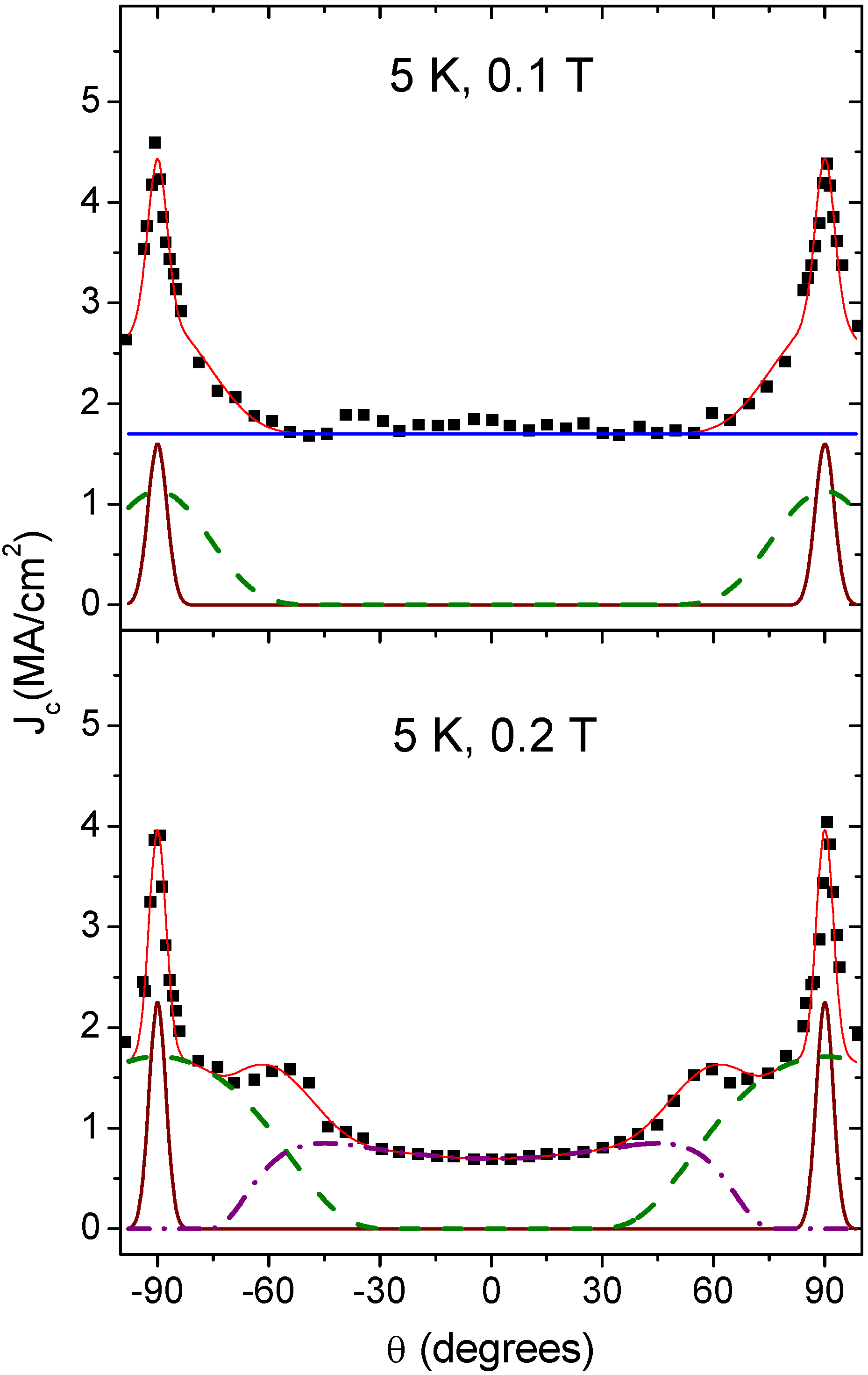
To illustrate this effect we show in Figure 5 a nanostructured LTS Nb film at two different field strengths. Experimental details of this sample are given elsewhere [9]. For both field strengths shown we are able to identify three components with parameters as shown in Table 1. The choice of components and fitting has been done “by eye” and with the assistance of a least squares fitting program. In principle this fitting and model selection should be done using a maximum entropy procedure such as outlined in [25] or other Bayesian model selection procedure.

This data shows two striking effects which can be accounted for by the maximum entropy description but are not predicted by any deterministic model. At 0.1 T, the angular dependence is flat around the region θ = 0°, despite the sample having correlated pinning structures oriented in this direction. From Equation (3c) we know it is possible for correlated pinning to give a flat angular response through the value γ = 1. At 0.2 T, we see the emergence of “shoulders” at θ ~ ±60°. It is difficult to foresee how a deterministic model would ever predict a J_c peak which is not aligned with the direction of correlated pinning, but this comes quite naturally from Equation (3b). Further examples of the use of these equations to explain J_c(θ) from complex pinning structures are given in [7,8,9,10,26,27].

Figure 5. J_c(θ) at 5 K for a nanostructured Nb thin film incorporating an array of vertical columnar pores: experiment (■), full fit ($▬$), fit components ($▬$, $▬ - ▬$, $▬ ▬ ▬$, $▬$). The fitting parameters for these data are summarized in Table 1.

Figure 5. J_c(θ) at 5 K for a nanostructured Nb thin film incorporating an array of vertical columnar pores: experiment (■), full fit ($▬$), fit components ($▬$, $▬ - ▬$, $▬ ▬ ▬$, $▬$). The fitting parameters for these data are summarized in Table 1.

Table 1. Parameters of fit components in Figure 5.

		0.1 T	0.2 T
Uniform ($▬$)	J0	5.33	―
Gaussian* ($▬ - ▬$)	J0	―	1.75
	σ	―	1.0
Gaussian ($▬ ▬ ▬$)	J0	0.65	1.93
	σ	0.23	0.45
Gaussian ($▬$)	J0	0.18	0.225
	σ	0.045	0.04

* Equation 3b shifted in phase by 90°.

Table 1. Parameters of fit components in Figure 5.

		0.1 T	0.2 T
Uniform ($▬$)	J0	5.33	―
Gaussian* ($▬ - ▬$)	J0	―	1.75
	σ	―	1.0
Gaussian ($▬ ▬ ▬$)	J0	0.65	1.93
	σ	0.23	0.45
Gaussian ($▬$)	J0	0.18	0.225
	σ	0.045	0.04

* Equation 3b shifted in phase by 90°.

3.4. Out-of-Plane Field Angular Dependence of J_c with Defects Oblique to the Crystal Axes

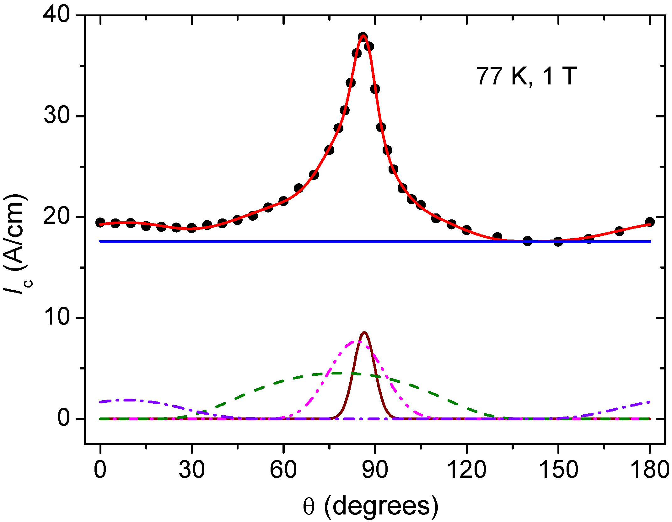
In some samples there exist extended defects at well-defined oblique angles to the crystal axes. These produce asymmetric J_c(θ) data. It is not obvious that these should continue to be described using constraints on cotθ. In Figure 6 we show results for a commercial sample of YBCO wire produced by SuperPower Inc. (Schenectady, NY, USA). These samples are known to have pinning structures at oblique angles. We find that this data can still be fitted by combinations of Equations (3a) and (3b) with allowance for shifting the center of the peaks. We discuss why the cotθ constraints may remain valid in Section 4.

Figure 6. J_c(θ) at 77 K, 1 T for a commercial YBCO wire from SuperPower Inc.; experiment (●), full fit ($▬$), fit components ($▬$, $▬$, $▬ - -$, $▬ ▬ ▬$, $▬ - ▬$). The fitting parameters for these data are summarized in Table 2. The center angle of each peak is also tabulated (NB. to fit Eqn. 3b substitute $\theta \to \theta -\pi /2+{\theta }_0$).

Figure 6. J_c(θ) at 77 K, 1 T for a commercial YBCO wire from SuperPower Inc.; experiment (●), full fit ($▬$), fit components ($▬$, $▬$, $▬ - -$, $▬ ▬ ▬$, $▬ - ▬$). The fitting parameters for these data are summarized in Table 2. The center angle of each peak is also tabulated (NB. to fit Eqn. 3b substitute $\theta \to \theta -\pi /2+{\theta }_0$).

Table 2. Parameters of fit components in Figure 6.

		1 T
Uniform ($▬$)	J0	55.3
Gaussian ($▬$)	J0	1.26
	σ	0.059
	θ0∗	86.4°
Gaussian ($▬ - -$)	J0	2.98
	σ	0.156
	θ0	83.8°
Gaussian ($▬ ▬ ▬$)	J0	5.01
	σ	0.44
	θ0	78.4°
Gaussian ($▬ - ▬$)	J0	1.35
	σ	0.29
	θ0	8.4°

* θ₀ is the center position of the peak.

Table 2. Parameters of fit components in Figure 6.

		1 T
Uniform ($▬$)	J0	55.3
Gaussian ($▬$)	J0	1.26
	σ	0.059
	θ0∗	86.4°
Gaussian ($▬ - -$)	J0	2.98
	σ	0.156
	θ0	83.8°
Gaussian ($▬ ▬ ▬$)	J0	5.01
	σ	0.44
	θ0	78.4°
Gaussian ($▬ - ▬$)	J0	1.35
	σ	0.29
	θ0	8.4°

* θ₀ is the center position of the peak.

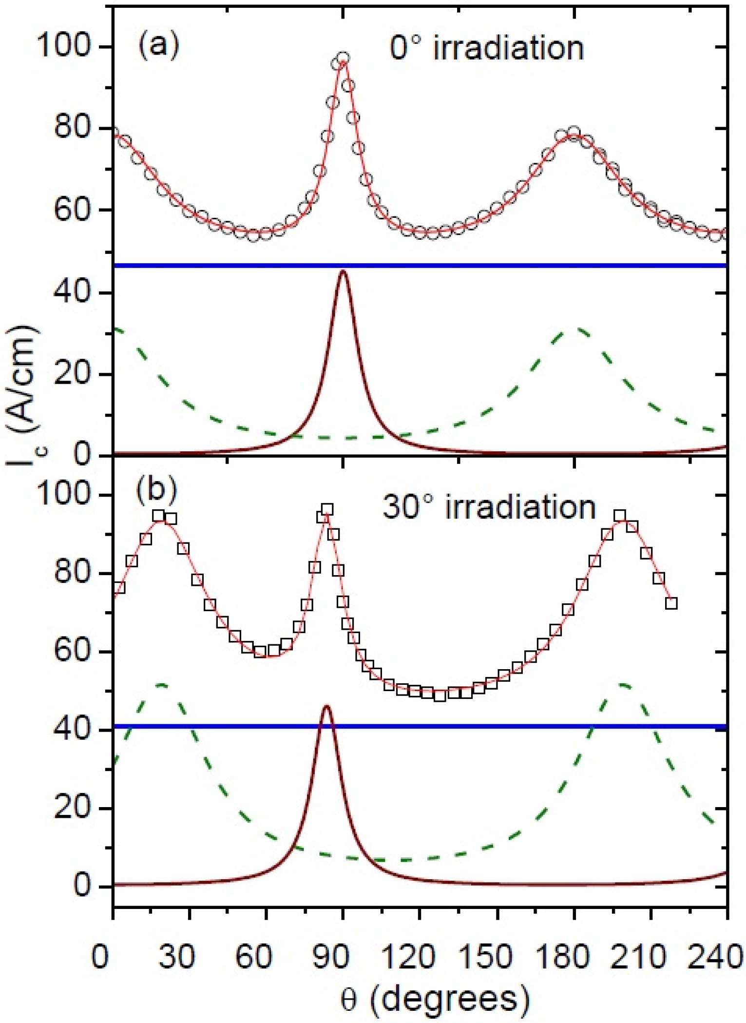
One way to controllably add extended defects at oblique angles is to use ion irradiation to create damage tracks through the films [28,29]. In Figure 7 we show the outcome of irradiating a YBCO thin film with ions at two different angles. The experimental details are published elsewhere [29]. In both cases there is a peak in J_c(θ) at θ = 90° due to the ab-plane stacking faults in the sample. The irradiation produces an additional peak approximately in the direction of the irradiation. This data can be fitted using a combination of Equations (3a) and (3c) with allowance for shifting the center of the peaks.

The conclusion from our analysis of data with oblique defects is that the maximum entropy distributions Equations (3a), (3b) and (3c) remain valid.

Figure 7. J_c(θ) at 77 K, 1 T for a YBCO thin film irradiated at (a) θ = 0°, (b) θ = 30° with Ag ions with areal density 10¹¹ cm⁻²; experiment (○,□), full fit ($▬$), fit components ($▬$, $▬$, $▬ ▬ ▬$). The fitting parameters for these data are summarized in Table 3. The center angle of each peak is also tabulated.

Figure 7. J_c(θ) at 77 K, 1 T for a YBCO thin film irradiated at (a) θ = 0°, (b) θ = 30° with Ag ions with areal density 10¹¹ cm⁻²; experiment (○,□), full fit ($▬$), fit components ($▬$, $▬$, $▬ ▬ ▬$). The fitting parameters for these data are summarized in Table 3. The center angle of each peak is also tabulated.

Table 3. Parameters of fit components in Figure 7.

Irradiation angle		0°	30°
Uniform ($▬$)	J0	146	129
Lorentzian ($▬$)	J0	17.2	17.68
	γ	0.12	0.12
	θ0	90°	83.6°
Lorentzian ($▬ ▬ ▬$)	J0	37.2	59.3
	γ	0.38	0.37
	θ0	0°	19.0°

Table 3. Parameters of fit components in Figure 7.

Irradiation angle		0°	30°
Uniform ($▬$)	J0	146	129
Lorentzian ($▬$)	J0	17.2	17.68
	γ	0.12	0.12
	θ0	90°	83.6°
Lorentzian ($▬ ▬ ▬$)	J0	37.2	59.3
	γ	0.38	0.37
	θ0	0°	19.0°

3.5. In-Plane Field Angular Dependence of J_c under Variable Lorentz Force

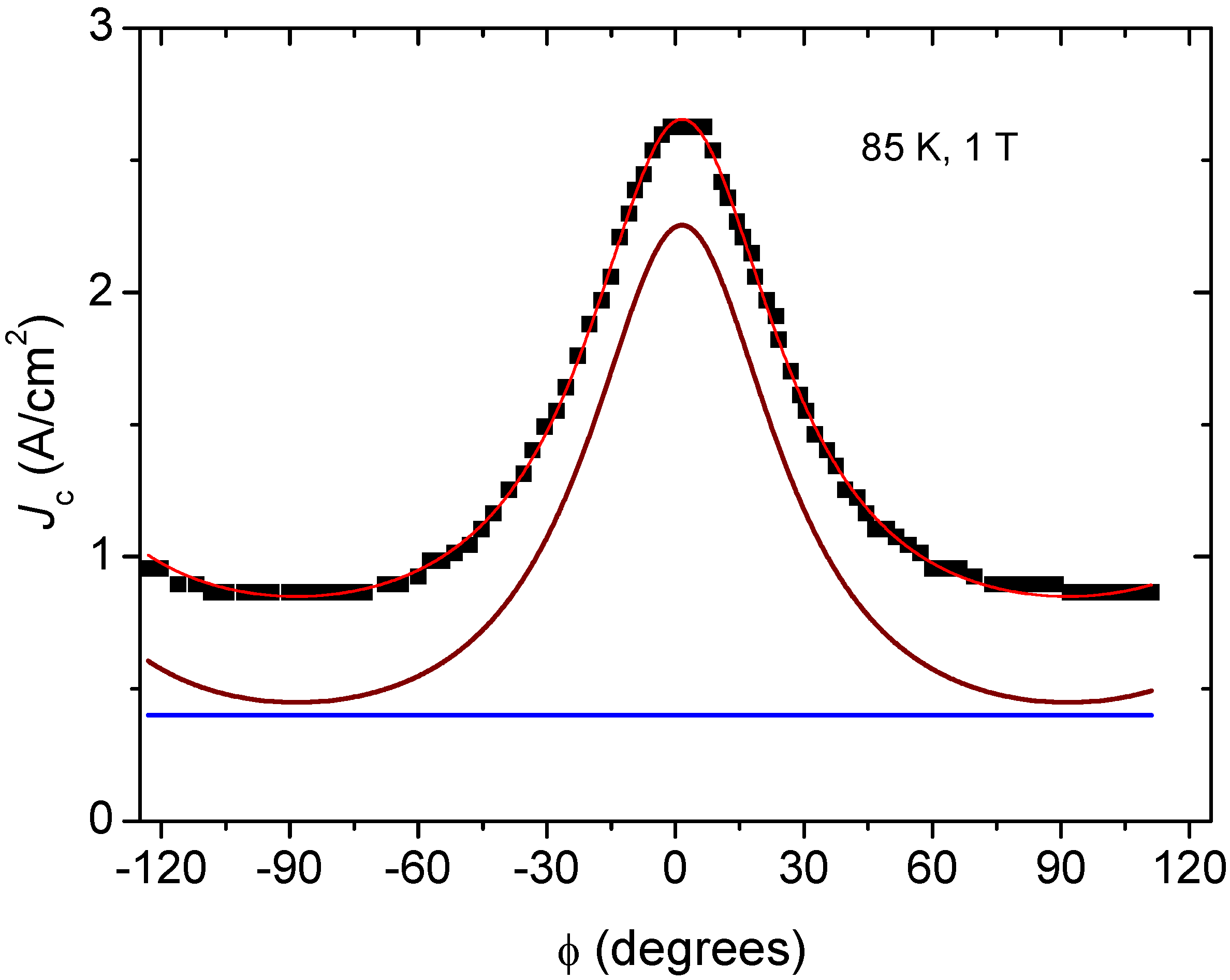
When the field direction is varied in a plane which includes the current direction then the Lorentz force experienced by the vortices varies as $J_{c}B\sin \varphi$. If we start from a force-based model it is therefore natural to attempt to include this variation in the model. As we consider the phenomenon from the point of view of maximum entropy, however, we are concerned with constraints, and it is not clear that the simple constraints we have proposed will alter just because the Lorentz force is varying. This in fact turns out to be the case. We have previously shown that combinations of Equations (3a), (3b) and (3c) can fit data for J_c(ϕ) [10]. In Figure 8 we show data for a YBCO sample measured at 85 K, 1 T [30]. The data is fitted with a combination of Equations (3a) and (3c); the peak has the angular-Lorentzian shape. The ability to describe J_c data for all arbitrary angles within the same theoretical framework is a particular strength of the maximum entropy approach. We discuss what this fitting implies for the vortex configurations for in-plane fields in Section 4.

Figure 8. J_c(ϕ) at 85 K, 1 T for a YBCO thin film of thickness 500 nm. Data from [30]; experiment (■), full fit ($▬$), fit components ($▬$,$▬$). The fitting parameters for these data are summarized in Table 4.

Figure 8. J_c(ϕ) at 85 K, 1 T for a YBCO thin film of thickness 500 nm. Data from [30]; experiment (■), full fit ($▬$), fit components ($▬$,$▬$). The fitting parameters for these data are summarized in Table 4.

Table 4. Parameters of fit components in Figure 8.

	1 T
Uniform ($▬$)	J0	1.25
Lorentzian ($▬$)	J0	3.16
	γ	0.45

Table 4. Parameters of fit components in Figure 8.

	1 T
Uniform ($▬$)	J0	1.25
Lorentzian ($▬$)	J0	3.16
	γ	0.45

3.6. Higher Order Constraints in J_c(θ)

The Equations (3a), (3b) and (3c), with suitable modifications, account for almost all J_c(θ) and J_c(ϕ) data in the literature. One exception is for samples which exhibit a phenomenon known as channeling. In this case there exists a preferred direction in which the vortices will move as there is only weak pinning available in this direction. An excellent model system for this effect are HTS films grown on vicinal-cut crystal substrates in which a force component on the vortices is directed along the ab-planes of the crystal [31,32]. The flux pinning is only weak in this direction as any effect of the intrinsic pinning or the pinning due to stacking faults within the layered structure is avoided.

Following the results of Carazza [23,24] we can consider the case where a fourth moment in z/y is defined. Carazza gives the solution $f(x)=1/(\alpha +\beta x^2+\gamma x^4)$ if only second and fourth moments in x are defined. Substituting z/y and transforming to the angular domain with the correct normalization gives:

$$J_{\text{c}}(\theta )=\frac{1}{2\pi }\frac{J_0\sqrt{A+2\sqrt{B}}}{{\cos }^2\theta +A{\sin }^2\theta +B{\sin }^2\theta {\tan }^2\theta }.$$

(3d)

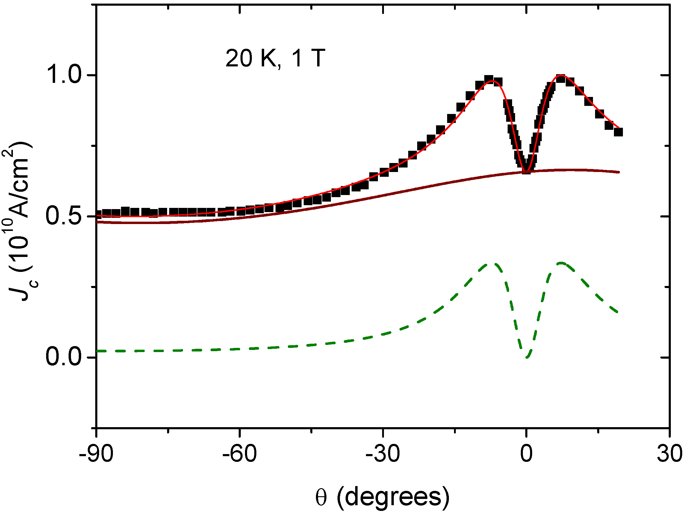
We call this an “angular quartic” distribution. In Figure 9 we have fitted data for a YBCO film on a vicinal substrate with a reported 4° miscut angle. The data can be fitted with two components, an angular Lorentzian with a peak centered at θ₀ = 5.3° and an angular quartic function centered at θ₀ = 0°. We are thus claiming that there exist two sets of constraints which affect the experiment. The effect of the channeling phenomenon is only present in one of these sets.

The physics of channeling is thus analogous to a random walk in a quartic potential in z/y. That is, the magnitude of the critical current at z/y is analogous to the probability of the position of a particle undergoing a random walk with position w = z/y. This is true to the extent that at high temperatures the quartic term effectively disappears and there is no channeling minimum in J_c [31,32].

Figure 9. J_c(θ) at 20 K, 1 T for a YBCO thin film grown on a vicinal substrate with a 4° miscut angle. Data from [31] experiment (■), full fit ($▬$), fit components ($▬$, $▬ ▬ ▬$). The fitting parameters for these data are summarized in Table 5.

Figure 9. J_c(θ) at 20 K, 1 T for a YBCO thin film grown on a vicinal substrate with a 4° miscut angle. Data from [31] experiment (■), full fit ($▬$), fit components ($▬$, $▬ ▬ ▬$). The fitting parameters for these data are summarized in Table 5.

Table 5. Parameters of fit components in Figure 9.

		1 T
Lorentzian ($▬$)	J0	1.76
	γ	0.85
	θ0	5.3
Quartic ($▬ ▬ ▬$)	J0	0.215
	Α	0.20
	Β	0.016
	θ0	0

Table 5. Parameters of fit components in Figure 9.

		1 T
Lorentzian ($▬$)	J0	1.76
	γ	0.85
	θ0	5.3
Quartic ($▬ ▬ ▬$)	J0	0.215
	Α	0.20
	Β	0.016
	θ0	0

4. Relating the Constraints to the Physics of Superconductors

In this section we discuss the connection between the chosen constraints and the physics of superconductors and hence the information available to the experimenter from the given experiments. We discuss what this tells us about the physics of pinning and how we should analyse experimental data of this type.

4.1. Temperature Constraints

Imagine an experiment measuring the critical current at temperature T. If, at an arbitrary time, we select a vortex at random, then this vortex will be either in state $S\equiv (\text{stationary vortex)}$, or state $M\equiv \text{ (moving vortex)}$. For a vortex chosen at random we have the binomial probabilities, $p(S)=p$, and $p(M)=1-p$, for finding the vortex in either state. If we change to a new temperature T’ then the probabilities will change $p(S)=p\text{'}$ and $p(M)=1-p\text{'}$. In this interpretation J_c(t) is proportional to a distribution of binomial probabilities, and the critical current is proportional to the fraction of pinned vortices. If the distributed quantity is a proportion or fraction then the only well-defined means are geometric means [33]. Thus $<\ln t>$ or $<\ln (1-t)>$ are possible simple constraints. Physically, T is an energy scale, and the energy scale relevant to pinning is the difference from the irreversibility temperature, $T_{irr}-T$. At T_irr the vortex lattice melts and forms a liquid state with no pinning of vortices. Hence, $<\ln (T_{irr}-T)>$, or using the reduced temperature, $<\ln (1-t)>$ is the relevant constraint. Physically this constraint refers to a geometric mean in pinning energy. This energy is $\delta E=k{T}_{irr}(1-\exp (<\ln (1-t)>))$. We interpret it as the geometric mean energy required to pin a vortex as this is the process we recognize as causing the distribution of J_c over temperature.

The energy scale associated with the line energy of a vortex is ${\epsilon }_0(t)\propto (1-t)$ [3]. Hence if$j_c(t)\propto (1-t)$ it is tempting to assert that only this energy scale is relevant to the temperature dependence [15]. This conclusion is not supported by a maximum entropy analysis. In our experiments such as shown in Figure 2, changes in the electronic doping state of YBCO which affect the superfluid density, or changes in microstructure which affect the density and type of pinning structures, cause a variation in the power law exponent. There is no reason to believe that at some unique value of electronic doping and for some particular microstructure only ${\epsilon }_0(t)$ is determining the properties, and for other settings of these variables other factors suddenly come into play.

A maximum entropy analysis of J_c(T) data involves fitting a mixture of power laws to the data. For each power law we have only an amplitude and exponent. A larger exponent implies the distribution of J_c(T) is weighted more heavily to low temperatures. These fitting parameters are the outcome of averaging over all physical factors which are determining J_c(T). If we alter some physical aspect of the sample such as increasing the density of one type of pinning structure and a fitting parameter changes then the correct conclusion is that the change is due to the altered pinning and how this affects vortex interactions with all the unaltered aspects of the sample. This may seem a pedantic point to the reader but it is not one which is generally considered by experimenters when analyzing J_c data. We have shown in our experiments with angular dependencies [9,16] that the same microstructure alterations can have radically different effects depending on pre-existing microstructures.

The information content of a single J_c(T) dataset is generally low. One way to acquire more information about the pinning in a sample would be to measure J_c(T) in a range of higher external fields. This may provide greater discrimination between the behavior of pinning populations with lower and higher densities.

4.2. Magnetic Field Constraints

The critical current at a particular field value is related to the proportion of pinned vortices, i.e., $J_c(B)\propto n_S(B)/B$. As with temperature we have a distributed quantity which is a proportion. Thus $<\ln b>$, and $<\ln (1-b)>$ are possible well defined simple constraints. The magnetic field fixes the total number of vortices in the sample via, $B=n{\varphi }_0$, where n is the areal density of vortices and ${\varphi }_0=h/2e$ is the magnetic flux quantum. Therefore, for a constraint to reflect a geometric mean in the total number of pinned vortices we should equalize the proportionality constant across all fields by multiplying by B. Thus we should form the beta distribution for flux pinning force, $F_p(b)~b^{\alpha -1}{(1-b)}^{\beta -1}$ and we have $<\ln b>=\mathrm{\Psi }(\alpha )-\mathrm{\Psi }(\alpha +\beta )$, where Ψ is the digamma function. The geometric mean number of stationary flux vortices is $n_S=(B_{irr}/{\varphi }_0)\exp (<\ln b>)$.

The interpretation of $<\ln (1-b)>$ is not obvious. The quantity $B_{irr}-B$ is the difference between the field and the maximum possible field or the maximum possible density of the vortex lattice for the superconductor under the experimental conditions. Hence, it can be thought of as a density of “vortex lattice vacancies” with respect to this maximum possible density. We therefore have a complementary constraint in the system in terms of a geometric mean, $<\ln (1-b)>$, of vortex lattice vacancies. These “vacancies” we are defining are not the same as the local vacancies, i.e. one missing vortex from a local triangular array, more commonly discussed in the superconductor literature [2]. At low fields we are essentially saying the whole sample consists of “vortex vacancies”. Whether there is additional insight to be gained from this point of view needs further consideration.

In Figure 3 we have shown that F_p(B) data for different angles can be scaled to a common curve. This procedure is also known to apply to LTS data as a function of temperature and strain [20]. At different angles the accommodation of the vortices to the pinning landscape in a Bi-2223 wire must be very different as it is a highly anisotropic material and the wire is well textured. It is quite remarkable that once we normalize the field domain [0, B_irr], the overall shape, defined by the exponents α and β, remains unchanged. This suggests that there are no absolute length scales which are important in determining this behavior as these would tend to favor particular values of vortex density, determined by B, or particular vortex cross sectional areas, determined by the orientation of the field, θ. The relative density of vortex “pancakes” and “strings”, which describe vortices in highly anisotropic superconductors such as Bi-2223, is also shown to be irrelevant. The retention of the same α, β, with temperature scaling, if it applies, shows that temperature is not altering any important relative length scales, or pinning potentials that determine the shape of F(b). In contrast it is known that changes in microstructure will alter the fitting parameters α, β, for some superconductors [1,20] and between different superconductors there are considerable variations.

The maximum entropy viewpoint informs us that α and β are connected to geometric means associated with pinning across the whole domain of 0 < b < 1. The persistence of particular values of α, β, shows these geometric means are relatively constant under many conditions. If the values of α and β do change with for example, microstructure variations, then as for the interpretation of J_c(T), the changes are due to how these variations have affected the whole pinning landscape, that is, the original structure in which they occur affects the outcome. Any interpretation of α or β as associated with one particular type of pinning defect or vortex lattice property is not credible in any real sample.

Finally, we note as an aside that the beta distribution is the conjugate prior for the binomial distribution in Bayesian statistical analysis. That is, a beta distribution is not altered in form when using Bayes theorem applied to data in the form of binomial outcomes. Hence, if we describe the state of our knowledge about our ensemble using a beta distribution, f(b), and then accumulate more information in the form of knowing whether a particular vortex is moving or stationary then the revised distribution, f’(b) remains a beta distribution. This is reassuring, even if we knew the state of every vortex in our sample, Bayes theorem tells us f(b) remains a beta distribution. An exception is if our system has multiple sets of constraints giving a mixture of beta distributions, in which case our choice of a single beta distribution as the prior is proved to be mistaken.

4.3. Field Angle Constraints

As stated earlier each pinned vortex i must have total pinned lengths (considering here for discussion purposes the θ variable) y_i and z_i. We can reason that if we know the ratio $z_i/y_i$ for all pinned vortices then we know f(θ) and the problem we set ourselves is solved. What maximum entropy has shown us is that we don’t need to know all $z_i/y_i$, merely the moments of $z/y$, in order to predict the forms of the distributions. From this viewpoint we have a classic example of the application of maximum entropy.

In earlier publications we derived Equations (3) by directly modeling the shape of the vortex path as a directed random walk [7,8]. That is for a peak centered in the y-direction, we modeled an arbitrarily chosen vortex as a finite set of m steps in the y-direction, giving say, $y=m\lambda$, where λ is the average step size in the y-direction. And then we let the alternating steps in the z-direction be chosen from a distribution, $N(z;\sigma )$,or $L(z;\gamma )$, which can be Gaussian or Lorentzian. This also leads to Equations (3) (with suitable adjustment of the scale parameters). This direct model of the vortex shape has the advantage that one can better interpret the physical meaning of the constraints. A distribution of correlated pinning defects of a single length scale is more likely to broaden a peak in a way which leads to an angular Gaussian distribution. That is, we can argue that the Gaussian distribution of the total pinned length in the z-direction is a result of the application of the central limit theorem as the total length is the result of summing lengths derived from distributions with finite variances. If we have many types of pinning defects with different length scales in the z-direction, then the vortex lengths in the z-direction are modeled by repeated sampling from $L(z;\gamma )$ and this does not give a convergence to a mean for $z/y$. That is, if we sample the values of $z_i/y_i$ from the ensemble of pinned vortices N times, then in the Gaussian case $<z/y>\to 0$ as $N\to \infty$ and the constraint $<z/y>=<\cot \theta >=0$ applies. If this sampling does not give a converging $<z/y>$, no constraint on the mean exists, and we get a broadening of a peak to an angular Lorentzian, or at least a peak shape derived from an approximation to a Lorentzian distribution in $z/y$; in reality it will be truncated at some value.

The magnitude of the scale constants for the angular distributions gives us a measure of the relative strength of the pinning populations in broadening a peak. That is, continuing with the y,z geometry as discussed with a peak in the y-direction, a large scale factor means pinning structures exist which relative to the y-direction pinning, can support a large pinned length in the z-direction. What is of some use to the experimenter is that these scale factors can be tracked as the field magnitude and temperature are changed. This gives some insight into the density and nature of the defects doing the pinning [9,16].

The weakness of a direct statistical model of the vortex such as described in [7,8] is it is difficult to understand how or if the model should be altered to take into account oblique defects or other additional forms of disorder. The maximum entropy approach relieves us of this burden as we can properly argue that if our distributions, derived from moments of $y/z$, accurately describe the data then adding further information to the model is unnecessary. Some insight into why the distributions remain unchanged for oblique defects can be gained by considering the infinite square lattice as a model leading to the prior uniform distribution for correlated pinning. If we rotate say the y-axis by the angle Ψ so that $y^{\prime }=y/\cos \mathrm{\Psi }$ then we still have a uniform distribution as previously with only a rescaled y variable. Likewise, such a rescaling may change the values of the constraints on the moments but not the form of the constraints.

The physical description of vortices when J//B and therefore ${\overrightarrow{F}}_p={\overrightarrow{J}}_c\times \overrightarrow{B}=0$ has long been of interest and remains an area of active research as the mechanism which limits the critical current in this configuration is not easily understood [2]. For example, a “force free torque” model has recently been proposed to explain the observed electric fields [34]. The fitting of J_c(ϕ) in Figure 8 into two components is therefore of particular interest. One of these components is an angular-Lorentzian. Applying our direct model of the vortex shape suggests that for this component the vortices have the structure of a directed random walk with steps aligned in the x-direction and alternating steps in the y-direction chosen from a Lorentz distribution. Our model doesn’t say anything about the structure in the z-direction. This model is therefore consistent with the idea that the vortex has a helical structure aligned macroscopically with the field, without being able to confirm this. The other component in J_c(ϕ) is uniform – that is the magnitude is not changed by the variable Lorentz force. This gives us no information about the vortex geometry.

4.4. Are Some Parameters in the Angular Fitting Redundant?

In Figure 5, Figure 6, Figure 7 and Figure 8 we notice that the extrema of different components sometimes coincide or nearly coincide in magnitude. For example, in Figure 9 the minima of the angular Lorenztian and the magnitude of the uniform component are close to equal. This effect was also noted in [9] as being quite a common occurrence when analyzing J_c(θ) data. A possible explanation is that there is a physical correlation between the pinning defects which are responsible for both components. If this coincidence is a real effect then it is possible to reduce the number of free parameters in the fitting. What these physical correlations may be is unclear in most cases. A coincidence of equal magnitude at some conditions for two or more fitting components implies that a pinned vortex has equal probability of being constrained by either set of the relevant constraints. This suggests that some application of the principle of maximum entropy may apply across the components of the mixture distributions.

5. Conclusions

Using maximum entropy inference is a novel approach to understanding critical currents in type II superconductors. The traditional approach to the phenomenon has been to construct deterministic models based on microscopic forces. The disorder which is inherent in real superconductors has either been ignored or incorporated through ad-hoc inclusions of statistical distributions describing the spatial arrangement of pinning defects. The deterministic models have been successful in elucidating much of the basic phenomenology however they have foundered when approaching problems such as pinning summation where we need to account for the multiplicity of ways a flux vortex may be pinned in a complex environment.

The maximum entropy approach gives a unified framework in which the dependence of critical currents on magnetic field, temperature and arbitrary field angle can be derived. The equations it yields have been shown to fit a large number of datasets in the literature. The approach has given maximum entropy expressions for angular data which have not been previously derived. These are able to explain non-intuitive experimental outcomes such as peaks in the critical current at angles which are intermediate between the known correlated defect directions. The constraints used in deriving the maximum entropy expressions can all be given physical interpretations which are consistent with the known microscopic physics.

Our analysis has revealed that the information available from a single dataset such as J_c(Β) or J_c(θ) is limited. This is compensated by the knowledge that tracking this information across a large range of conditions is a sound method for untangling the very complex behavior of the critical currents of superconductors.

References

- Matsushita, T. Flux Pinning in Superconductors; Springer: Berlin, Germany, 2006. [Google Scholar]
- Campbell, A.M.; Evetts, J.E. Critical Currents in Superconductors; Taylor & Francis: London, UK, 1972. [Google Scholar]
- Blatter, G.; Feigel’man, M.V.; Geshkenbein, V.B.; Larkin, A.I.; Vinokur, V. M. Vortices in high temperature superconductors. Rev. Mod. Phys. 1994, 66, 1125–1388. [Google Scholar] [CrossRef]
- Hao, Z.; Clem, J.R. Angular dependences of the thermodynamic and electrodynamic properties of the high-Tc superconductors in the mixed state. Phys. Rev. B 1992, 46, 5843–5847. [Google Scholar] [CrossRef]
- Keys, S.A.; Hampshire, D.P. Characterization of the transport critical current density for conductor applications. In Handbook of Superconducting Materials; Cardwell, D.A., Ginley, D.S., Eds.; Institute of Physics Publishing Ltd.: Bristol, UK, 2003; pp. 1297–1322. [Google Scholar]
- Anderson, P.W. Theory of flux creep in hard superconductors. Phys. Rev. Lett. 1962, 9, 309–311. [Google Scholar] [CrossRef]
- Long, N.J.; Strickland, N.; Talantsev, E.F. Modelling of vortex paths in HTS. IEEE Trans. Appl. Supercond. 2007, 17, 3684–3687. [Google Scholar] [CrossRef]
- Long, N.J. Model for the angular dependence of critical currents in technical superconductors. Supercond. Sci. Technol. 2008, 21, 025007. [Google Scholar] [CrossRef]
- Wimbush, S.C.; Long, N.J. The interpretation of the field angle dependence of the critical current in defect-engineered superconductors. New J. Phys. 2012, 14, 083017. [Google Scholar] [CrossRef]
- Long, N.J. A statistical mechanical model of critical currents in superconductors. J. Supercond. Nov. Magn. 2013. [Google Scholar] [CrossRef]
- Jaynes, E.T. Information theory and statistical mechanics. Phys. Rev. 1957, 106, 620–630. 1957, 108, 171–190. [Google Scholar] [CrossRef]
- Kapur, J.N. Maximum-Entropy Models in Science and Engineering, 2nd ed.; New Age: New Delhi, India, 2009. [Google Scholar]
- Jaynes, E.T. Where do we stand on Maximum Entropy? In The Maximum Entropy Formalism; Levine, R.D., Tribus, M., Eds.; MIT Press: Cambridge, MA, 1978; pp. 15–118. [Google Scholar]
- Jung, J.; Yan, H.; Darhmaoui, H.; Abdelhadi, M.; Boyce, B.; Lemberger, T. Universal relationship between critical currents and nanoscopic phase separation in high-Tc thin films. Supercond. Sci. Technol. 1999, 12, 1086–1089. [Google Scholar] [CrossRef]
- Albrecht, J.; Djupmyr, M.; Bruck, S. Universal temperature scaling of flux line pinning in high-temperature superconducting thin films. J. Phys.: Condens. Matter 2007, 19, 216211. [Google Scholar] [CrossRef]
- Long, N.J.; Wimbush, S.C.; Strickland, N.M.; Talantsev, E.F.; D’Souza, P.; Xia, J.A.; Knibbe, R. Relating critical currents to defect populations in superconductors. IEEE Trans. Appl. Supercond. 2013, 23, 8001705. [Google Scholar] [CrossRef]
- Fietz, W.A.; Webb, W.W. Hysteresis in superconducting alloys—Temperature and field dependence of dislocation pinning in niobium alloys. Phys. Rev. 1969, 178, 657–667. [Google Scholar]
- Kramer, J. Scaling laws for flux pinning in hard superconductors. J. Appl. Phys. 1973, 44, 1360–1371. [Google Scholar] [CrossRef]
- Varanasi, C.V.; Barnes, P.N. High Temperature Superconductors; Bhattacharya, R., Paranthaman, M.P., Eds.; Wiley-VCH: Weinheim, Germany, 2010; pp. 105–127. [Google Scholar]
- Ekin, J.W. Unified scaling law for flux pinning in practical superconductors: I. Separability postulate, raw scaling data and parameterization at moderate strains. Supercond. Sci. Technol. 2010, 23, 083001. [Google Scholar] [CrossRef]
- Specht, E.D.; Goyal, A.; Li, J.; Martin, P. M.; Li, X.; Rupich, M.W. Stacking faults in YBa2Cu3O7−x: Measurement using x-ray diffraction and effects on critical current. Appl. Phys. Lett. 2006, 89, 162510. [Google Scholar] [CrossRef]
- Van der Beek, C.J.; Konczykowski, M.; Prozorov, R. Anisotropy of strong pinning in multi-band superconductors. Supercond. Sci. Technol. 2012, 25, 084010. [Google Scholar] [CrossRef] [Green Version]
- Carazza, B.; Casaktelli, M. Deduction of the Lorentzian shape from maximum-entropy principle. Lett. Nuovo Cimento Series 2 1977, 20, 666–668. [Google Scholar] [CrossRef]
- Carazza, B. On the Lorentzian shape and the information provided by an experimental plot. J. Phys. A: Math. Gen. 1976, 9, 1069–1072. [Google Scholar] [CrossRef]
- Davies, S.; Packer, K.J.; Baruya, A.; Grant, A.I. Enhanced information recovery in spectroscopy using the maximum entropy method. In Maximum Entropy in Action; Buck, B., Macaulay, V.A., Eds.; Oxford University Press: Oxford, UK, 1990; pp. 73–107. [Google Scholar]
- Mikheenko, P.; Dang, V-S.; Tse, Y.Y.; Awang Kechik, M.M.; Paturi, P.; Huhtinen, H.; Wang, Y.; Sarkar, A.; Abell, J.S.; Crisan, A. Integrated nanotechnology of pinning centers in YBa2Cu3Ox films. Supercond. Sci. Technol. 2010, 23, 125007. [Google Scholar] [CrossRef]
- Paturi, P. The vortex path model and angular dependence of Jc in thin YBCO films deposited from undoped and BaZrO3-doped targets. Supercond. Sci. Technol. 2010, 23, 025030. [Google Scholar] [CrossRef]
- Civale, L.; Marwick, A.D.; Worthington, T.K.; Kirk, M.A.; Thompson, J.R.; Krusin-Elbaum, L.; Sun, Y.; Clem, J.R.; Holtzberg, F. Vortex confinement by columnar defects in YBa2Cu3O7 crystals: Enhanced pinning at high fields and temperatures. Phys. Rev. Lett. 1991, 67, 648–651. [Google Scholar] [CrossRef] [PubMed]
- Strickland, N.M.; Long, N.J.; Xia, J.; Kennedy, J.; Markwitz, A.; Zondervan, A.; Rupich, M.W.; Zhang, W.; Li, X.; Kodenkandath, T.; et al. Enhanced flux pinning in MOD second generation HTS wires by silver- and copper-ion irradiation applied superconductivity. IEEE Trans. Appl. Supercond. 2007, 17, 3306–3309. [Google Scholar] [CrossRef]
- Clem, J.R.; Weigand, M.; Durrell, J.H.; Campbell, A.M. Theory and experiment testing flux-line-cutting physics. Supercond. Sci. Technol. 2011, 24, 062002. [Google Scholar] [CrossRef]
- Durrell, J.H. Critical Current Anisotropy in High Temperature Superconductors. Ph.D. Thesis, University of Cambridge, UK, 2001. Available online: http://www.dspace.cam.ac.uk/bitstream/1810/34606/1/John%20Durrell.pdf (accessed on 30 Decvember 2012). [Google Scholar]
- Durrell, J.H.; Burnell, G.; Barber, Z.H.; Blamire, M.G.; Evetts, J.E. Critical currents in vicinal YBa2Cu3O7−δ films. Phys. Rev. B 2004, 70, 214508–214517. [Google Scholar] [CrossRef]
- Fleming, P.J.; Wallace, J.J. How not to lie with statistics: The correct way to summarize benchmark results. Commun. ACM 1986, 29, 218–221. [Google Scholar] [CrossRef]
- Matsushita, T. Longitudinal magnetic field effect in superconductors. Jap. J. Appl. Phys. 2012, 51, 010111. [Google Scholar] [CrossRef]
© 2013 by the authors; licensee MDPI, Basel, Switzerland. This article is an open access article distributed under the terms and conditions of the Creative Commons Attribution license (http://creativecommons.org/licenses/by/3.0/).
Share and Cite
MDPI and ACS Style
Long, N.J. Maximum Entropy Distributions Describing Critical Currents in Superconductors. Entropy 2013, 15, 2585-2605. https://doi.org/10.3390/e15072585
AMA Style
Long NJ. Maximum Entropy Distributions Describing Critical Currents in Superconductors. Entropy. 2013; 15(7):2585-2605. https://doi.org/10.3390/e15072585
Chicago/Turabian StyleLong, Nicholas J. 2013. "Maximum Entropy Distributions Describing Critical Currents in Superconductors" Entropy 15, no. 7: 2585-2605. https://doi.org/10.3390/e15072585