Correlation Distance and Bounds for Mutual Information

Centre for Quantum Computation and Communication Technology (Australian Research Council), Centre for Quantum Dynamics, Griffith University, Brisbane, QLD 4111, Australia
Entropy 2013, 15(9), 3698-3713; https://doi.org/10.3390/e15093698
Submission received: 21 June 2013
/
Revised: 21 August 2013
/
Accepted: 3 September 2013
/
Published: 6 September 2013
(This article belongs to the Special Issue Distance in Information and Statistical Physics Volume 2)
Abstract
:The correlation distance quantifies the statistical independence of two classical or quantum systems, via the distance from their joint state to the product of the marginal states. Tight lower bounds are given for the mutual information between pairs of two-valued classical variables and quantum qubits, in terms of the corresponding classical and quantum correlation distances. These bounds are stronger than the Pinsker inequality (and refinements thereof) for relative entropy. The classical lower bound may be used to quantify properties of statistical models that violate Bell inequalities. Partially entangled qubits can have lower mutual information than can any two-valued classical variables having the same correlation distance. The qubit correlation distance also provides a direct entanglement criterion, related to the spin covariance matrix. Connections of results with classically-correlated quantum states are briefly discussed.
Keywords:
mutual information; variational distance; trace distance; Pinsker inequality; quantum entanglementClassification:
PACS 89.70.Cf; 03.67.-a.1. Introduction
The relative entropy between two probability distributions has many applications in classical and quantum information theory. A number of these applications, including the conditional limit theorem [1], quantum error correction [2], and secure random number generation and communication [3,4], make use of lower bounds on the relative entropy in terms of a suitable distance between the two distributions. The best known such bound is the so-called Pinsker inequality [5]
where is the variational or L1 distance between distributions P and Q. Note that the choice of logarithm base is left open throughout this paper, corresponding to a choice of units. There are a number of such bounds [5], all of which easily generalise to the case of quantum probabilities [2,6,7].
However, in a number of applications of the Pinsker inequality and its quantum analog, a lower bound is in fact only needed for the special case that the relative entropy quantifies the mutual information between two systems. Such applications include, for example, secure random number generation and coding [3,4] (both classical and quantum), and quantum de Finnetti theorems [8]. Since mutual information is a special case of relative entropy, it follows that it may be possible to find strictly stronger lower bounds for mutual information.
Surprisingly little attention appears to have been paid to this possibility of better lower bounds (although upper bounds for mutual information have been investigated [9]). The results of preliminary investigations are given here, with explicit tight lower bounds being obtained for pairs of two-valued classical random variables, and for pairs of quantum qubits with maximally-mixed reduced states.
In the context of mutual information, the corresponding variational distance reduces to the distance between the joint state of the systems and the product of their marginal states, referred to here as the “correlation distance”. It is shown that both the classical and quantum correlation distances are relevant for quantifying properties of quantum entanglement: the former with respect to the classical resources required to simulate entanglement, and the latter as providing a criterion for qubit entanglement. In the quantum case, it is also shown that the minimum value of the mutual information can only be achieved by entangled qubits if the correlation distance is more than ≈.
The main results are given in the following section. Lower bounds on classical and quantum mutual information for two-level systems are derived in Section 3 and Section 5, and an entanglement criterion for qubits in terms of the quantum correlation distance is obtained in Section 4. Connections with classically-correlated quantum states are briefly discussed in Section 6, and conclusions are presented in Section 7.
2. Definitions and Main Results
For two classical random variables A and B, with joint probability distribution and marginal distributions and , the Shannon mutual information and the classical correlation distance are defined respectively by
where denotes the Shannon entropy of distribution P. The term “correlation distance” is used for , since it inherits all the properties of a distance from the more general variational distance, and clearly vanishes for uncorrelated A and B. Both the mutual information and correlation distance have a minimum value of zero, and for n-valued random variables have maximum values
with saturation corresponding to the maximally correlated case . Note for that .
For two quantum systems A and B described by density operator and reduced density operators and , the corresponding quantum mutual information and quantum correlation distance are analogously defined by
where denotes the von Neumann entropy of density operator ρ. Similarly to the classical case, these are direct measures of the correlation between A and B, vanishing only for uncorrelated A and B. It may be noted that trace distance has recently also been used to distinguish between and quantify quantum and classical contributions to this correlation [10,11]. For n-level quantum systems one has the maximum values
with saturation corresponding to maximally entangled states. Thus, comparing with Equation (4), quantum correlations have a quadratic advantage with respect to both mutual information and correlation distance. For example, for one has , allowing quantum correlation distances that are greater than the corresponding classical maximum value of unity.
In both the classical and quantum cases, one has the lower bound
for mutual information, as a direct consequence of the Pinsker inequality (1) for classical relative entropies [2,5,6,7]. However, better bounds for mutual information can be obtained, which are stronger than any general inequality for relative entropy and variational distance.
For example, for two-valued classical random variables A and B one has the tight lower bound
for classical mutual information. This inequality has been previously stated without proof in Reference [12], where it was used to bound the shared information required to classically simulate entangled quantum systems. It is proved in Section 3 below.
In contrast to Pinsker-type inequalities such as Equation (8), the quantum generalisation of Equation (9) is not straightforward. In particular, note for a two-qubit system that one cannot simply replace by in Equation (9), as the right hand side would be undefined for . This can occur if the qubits are entangled. Indeed, as shown in Section 4, is a sufficient condition for the entanglement of two qubits, as is the stronger condition
An explicit expression for the quantum correlation distance for two qubits, in terms of the spin covariance matrix, is also given in Section 4.
It is shown in Section 5 that the quantum equivalent of Equation (9), i.e., a tight lower bound for the quantum mutual information shared by two qubits, is
when the reduced density operators are maximally mixed, where corresponds to the value of for which the two expressions are equal. For this lower bound can only be achieved by entangled states, and cannot be achieved by any classical distribution having the same correlation distance. It is also shown that, for , the bound is also tight if only one of the reduced states is maximally mixed. Support is given for the conjecture that the bound in Equation (11) in fact holds for all two-qubit states.
In Section 6 the natural role of “classically-correlated” quantum states, in comparing classical and quantum correlations, is briefly discussed. Such states have the general form [13], where is a classical joint probability distribution and and are orthonormal basis sets for the two quantum systems. The lower bound in Equation (11) can be saturated by a classically-correlated state if and only if .
3. Tight Lower Bound for Classical Mutual Information
3.1. Derivation of Bound
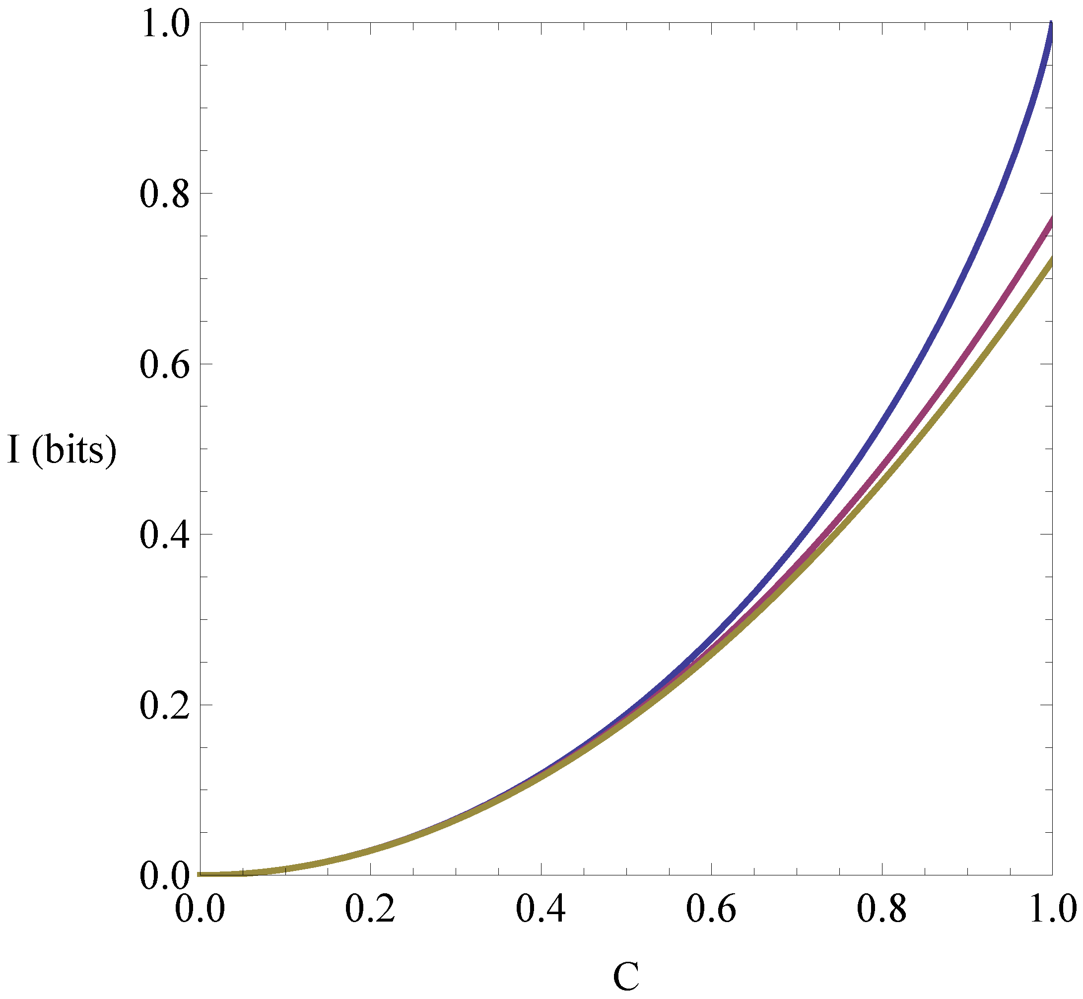
The tight lower bound in Equation (9) is derived here. The bound is plotted in Figure 1 below (top curve). Also plotted for comparison are the Pinsker lower bound in Equation (8) (bottom curve), and the lower bound following from the best possible generic inequality for relative entropy and variational distance, given in parametric form in Reference [5] (middle curve).
To derive the bound in Equation (9), it is convenient to label the two possible values of A and B by . Defining , it follows by summing over each of a and b separately that , implying that with . Hence, . Further, writing and , for suitable , the positivity condition is equivalent to
Now, Equation (9) is equivalent to
It is easy to check that this inequality is always saturated for the case of maximally-random marginals, i.e., when . In all other cases, the inequality may be proved by showing that has a unique global minimum value of 0 at .
Figure 1.
Lower bounds for the classical mutual information between two-valued variables.
In particular, note first that (one has in this case, so that the mutual information vanishes). Further, using , one easily calculates that, using logarithm base e for convenience,
Hence, if and only if the argument of the logarithm is unity, i.e., if and only if
Expanding and simplifying yields two possible solutions: , or . However, in the latter case one has
where α and γ denote the arithmetic mean and geometric mean, respectively, of and (hence ). This is clearly inconsistent with the positivity condition (12) (unless , which trivially saturates Equation (13) for all r as noted above). The only remaining solution to is then , implying has a unique maximum or minimum value at . Finally, it is easily checked that it is a minimum, since
(with equality only for the trivially-saturating case ). Thus, as required.
3.2. Application: Resources for Simulating Bell Inequality Violation
The hallmark feature of quantum correlations is that they cannot be explained by any underlying statistical model that satisfies three physically very plausible properties: (i) no signaling faster than the speed of light; (ii) free choice of measurement settings; and (iii) independence of local outcomes. Various interpretations of quantum mechanics differ in regard to which of these properties should be given up. It is of interest to consider by how much they must be given up, in terms of the information-theoretic resources required to simulate a given quantum correlation [14]. For example, how many bits of communication, or bits of correlation between the source and the measurement settings, or bits of correlation between the outcomes, are required? The lower bound for classical mutual information in Equation (9) is relevant for the last of these questions.
In more detail, if denotes the joint probability of outcomes a and b, for measurements of variables A and B on respective spacelike-separated systems, and λ denotes any underlying variables relevant to the correlations, then Bayes theorem implies that
where summation is replaced by integration over any continuous values of λ. The no-signaling property requires that the underlying marginal distribution of A, , is independent of whether B or was measured on the second system (and vice versa), while the free-choice property requires that λ is independent of the choice of the measured variables A and B, i.e., that for any . Finally, the outcome independence property requires that any observed correlation between A and B arises from ignorance of the underlying variable, i.e., that for all A, B and λ. Thus the correlation distance of vanishes identically:
As is well known, the assumption of all three properties implies that two-valued random variables with values must satisfy the Bell inequality [15]
whereas quantum correlations can violate this inequality by as much as a factor of [16]. It follows that quantum correlations can only be modeled by relaxing one or more of the above properties, as has recently been reviewed in detail in Reference [12].
For example, assuming that no-signaling and measurement independence hold (as they do in the standard Copenhagen interpretation of quantum mechanics), and defining to be the maximum value of over all A, B and λ, it can be shown that Equation (20) generalises to the tight bound [12]
It follows that to simulate a Bell inequality violation , for some , the observers must share random variables having a correlation distance of at least . Hence, using the classical lower bound Equation (9) (stated without proof in Reference [12]), the observers must share a minimum mutual information of
Note this reduces to zero in the limit of no violation of Bell inequality (20), i.e., when , and reaches a maximum of 1 bit of information in the limit of the maximum possible violation over arbitrary probability distributions, . To simulate the maximum quantum violation [16], i.e., , at least 0.264 bits are required.
4. Quantum Correlation Distance and Qubit Entanglement
The positivity condition (12) may be used to show that the classical correlation distance between any pair of two-valued random variables is never greater than unity, i.e., that [12]. In contrast, the quantum correlation distance between a pair of qubits can be greater than unity, with upper bound , as per Equation (7).
Non-classical values of the quantum correlation distance are closely related to the quintessential non-classical feature of quantum mechanics: entanglement. In particular, is a direct signature of qubit entanglement. Indeed, even correlation distances smaller than unity can imply two qubits are entangled, as per the criterion given in Equation (10) and shown below. An explicit formula for qubit correlation distance in terms of the spin covariance matrix, needed for Section 5, is also obtained below.
4.1. Entanglement Criterion
Recall that the density operator of two qubits may always be written in the Fano form [17]
Here I is the unit operator; denotes the set of Pauli spin observables on each qubit Hilbert space; the components of the 3-vectors u and v are the spin expectation values and , for A and B respectively; and T denotes the spin covariance matrix with coefficients
It immediately follows from Equation (23) that the quantum correlation distance may be expressed in terms of the spin covariance matrix as
This expression will be further simplified in Section 4.2.
Now consider the case where is a separable state, i.e., of the unentangled form
for some probability distribution and local density operators , . Defining , implies and , and substitution into Equation (25) then yields
Note that second line follows from the properties and of the trace norm [18]; the third line using and the Schwarz inequality; and the last line via .
Equation (27) holds for all separable qubit states. Hence, a non-classical value of the correlation distance, , immediately implies that the qubits must be entangled. More generally, noting that and , one has , , and the stronger entanglement criterion (10) immediately follows from Equation (27).
The fact that entanglement between two qubits is necessary (but not sufficient) for to be greater than the maximum possible value of , for two-valued classical variables, is a nice distinction between quantum and classical correlation distances. It would be of interest to determine whether this result generalises to n-level systems. This would follow from the validity of Equation (10) for arbitrary quantum systems.
4.2. Explicit Expression for
To explicitly evaluate in Equation (25), let denote a singular value decomposition of the spin covariance matrix. Thus, K and L are real orthogonal matrices and , with the singular values corresponding to the square roots of the eigenvalues of . Noting that any orthogonal matrix is either a rotation matrix, or the product of a rotation matrix with the parity matrix , one therefore always has a decomposition of the form where K and L are now restricted to be rotation matrices. Hence, defining unitary operators U and V corresponding to rotations K and L, via and , and using the invariance of the trace norm under unitary transformations, the quantum correlation distance in Equation (25) can be rewritten as
Determining the eigenvalues of the Hermitian operator is a straightforward matrix calculation using the standard representation of the Pauli sigma matrices. Summing the absolute values of these eigenvalues then yields the explicit expression
for the quantum correlation distance, in terms of the singular values of the spin covariance matrix.
For example, for the Werner state , where is the singlet state and [19], one has and hence that . The corresponding correlation distance is therefore , which is greater than the classical maximum of unity for .
Equation (29) also allows the qubit entanglement criterion (10) to be directly compared with the strongest known criterion based on the spin covariance matrix [20]:
For the above Werner state this criterion is tight, indicating entanglement for . Hence, the main interest in weaker entanglement criteria based on quantum correlation distance lies in their direct connection with non-classical values of the classical correlation distance.
5. Tight Lower Bound for Quantum Mutual Information
Here Equation (11) is derived for the case . Evidence is provided for the conjecture that Equation (11) in fact holds for all two-qubit states, including a partial generalisation of Equation (11) when only one of and is maximally-mixed.
5.1. Derivation for Maximally-Mixed and
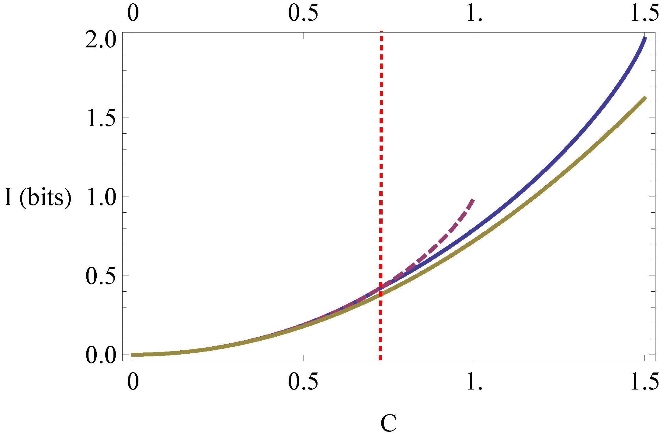
The tight lower bound for quantum mutual information in Equation (11), for maximally-mixed reduced states, is plotted in Figure 2 below (top solid curve). Also plotted for comparison are the Pinsker lower bound in Equation (8) (bottom solid curve), and classical lower bound in Equation (9) (dashed curve). The dotted vertical line indicates the value of in Equation (11). It is seen that quantum correlations can violate the classical lower bound for correlation distances falling between and 1.
To derive Equation (11) for , note first that Equation (23) reduces to . By the same argument given in Section 4.2, this can be transformed via local unitary transformations to the state
where , , and are the singular values of the spin covariance matrix T. Since the quantum mutual information and quantum correlation distance are invariant under local unitary transformations, one has and . Hence Equation (11) only needs to be demonstrated for .
Figure 2.
Lower bounds for the quantum mutual information between two qubits.

The mutual information of is easily evaluated as
where , , , are the eigenvalues of . Inverting the relation between the and further yields
and hence the correlation distance follows from Equation (29) as
Equation (32) implies that a tight lower bound for corresponds to a tight upper bound for . To determine the maximum value of , for a fixed correlation distance C, consider first the case . The ordering and positivity conditions on then require
(implying ). Further, from Equation (34), . Hence, if , then , implying the constraint . Noting the concavity of entropy, the maximum possible entropy under this constraint corresponds to equal values
(which are compatible with the above conditions on the ). Conversely, if then , and hence is fixed, implying by concavity that the maximum possible entropy corresponds to
(which again satisfies the required conditions on the ). It follows that the maximum possible entropy is (i) the maximum of the entropies
for , and (ii) for . However, it is straightforward to show that over their overlapping range. Hence the maximum possible entropy is always for the case .
For the case , the conditions on require that
(implying ), while from Equation (34) . Carrying out a similar analysis to the above, one finds that the maximum possible entropy is (i) the maximum of the entropies and
for , and (ii) for .
Numerical comparison shows that for , and otherwise. Hence, from Equation (32) one has the tight lower bound
Since , it follows that Equation (11) holds for in Equation (31), and hence for all qubit states with maximally-mixed reduced density operators, as claimed.
The states saturating the lower bound in Equations (11) and (42) are easily constructed from the above derivation. In particular, they are given by
and any local unitary transformations thereof, where the quantum correlation distance of is C by construction.
Note that is unentangled for (it can be written as a mixture of , and , where ). Conversely, is an entangled Werner state for (with singlet state weighting ). Hence, the lower bound in Equations (11) and (42) can only be achieved by entangled states for , and cannot be achieved by any two-valued classical random variables.
5.2. Conjecture
It is conjectured that Equation (11) is in fact a tight lower bound for any two-qubit state. This conjecture would follow immediately if it could be shown that
for arbitrary , where , and where it must further be shown that is a density operator. The conjecture would then follow since is of the form of in Equation (31), and hence satisfies Equation (42).
Partial support for Equation (44), and hence for the conjecture, is given by noting that any and corresponding can be brought to the respective forms
via suitable local unitary transformations, similarly to the argument in Section 4.2. Defining the function
it is straightforward to show that and for , consistent with . However, it remains to be shown that the gradient does not vanish for other physically possible values of (other than for the trivially saturating case ).
The above conjecture is further supported by the generalisation of Equation (11) in the following section.
5.3. Generalisation to Maximally-Mixed or
It is straightforward to show that the lower bound on quantum mutual information is tight for when just one of the mixed density operators is mixed, i.e., if or is equal to .
First, since is invariant under unitary transformations, the same argument as in Section 4.2 implies the state can always be transformed by local unitary transformations to the generalised form
of Equation (31), where either or equals and .
Second, let denote the “twirling” operation, corresponding to applying a random unitary transformation of the form [21]. It is easy to check that by definition , and , for any j and k. Since Werner states are invariant under twirling [19,21], it follows that . Using these properties, one finds that if one of or is maximally mixed, and hence that
where and the second equality holds for (but not otherwise), with defined as per Equation (43). Further, from Equation (29) one has
Recalling that saturates Equation (42), an analysis similar to Section 5.1 shows for that
with equality for .
Third, again using , and the property that the relative entropy is non-increasing under the twirling operation, it follows that
for . Since Werner states are invariant under twirling, this inequality is tight for , being saturated by the choice . Recalling that mutual information and correlation distance are invariant under local unitary operations, the inequality is therefore tight for any for which one of and is maximally mixed, as claimed.
6. Classically-Correlated Quantum States
It is well known that a quantum system behaves classically if the state and the observables of interest all commute, i.e., if they can be simultaneously diagonalised in some basis. Hence, a joint state will behave classically if the relevant observables of each system commute with each other and the state. It is therefore natural to define to be classically correlated if and only if it can be diagonalised in a joint basis [13], i.e., if and only if
for some distribution and orthonormal basis set . Classical correlation is preserved by tensor products, and by mixtures of commuting states.
While, strictly speaking, a classically-correlated quantum state only behaves classically with respect to observables that are diagonal with respect to , they also have a number of classical correlation properties with respect to general observables [13,22], briefly noted here.
First, above is separable by construction, and hence is unentangled. Second, since it is diagonal in the basis , the mutual information and correlation distance are easily calculated as
and hence can only take classical values.
Third, if M and N denote any observables for systems A and B respectively, then their joint statistics are given by
where is a stochastic matrix with respect to its first and second pairs of indices. Similarly, one finds
for the product of the marginals. Since the classical relative entropy and variational distance can only decrease under the action of a stochastic matrix, it follows that one has the tight inequalities [13,22]
with saturation for M and N diagonal in the bases and respectively. Maximising the first of these equalities over M or N immediately implies the well-known result that classically-correlated states have zero quantum discord [22].
Finally, for two-qubit systems, Equation (52) implies that is classically correlated if and only if it is equivalent under local unitary transformations to a state of the form
where and r satisfies Equation (12). Hence, the mutual information is bounded by the classical lower bound in Equation (9), and in Equation (43) is classically correlated for . It follows that the lower bound for quantum mutual information in Equation (11) can be attained by classically-correlated states if . Conversely, the minimum possible bound cannot be reached by any classically-correlated two-qubit state if .
7. Conclusions
Lower bounds for mutual information have been obtained that are stronger than those obtainable from general bounds for relative entropy and variational distance. Unlike the Pinsker inequality in Equation (8), the quantum form of these bounds is not a simple generalisation of the classical form.
Similarly to the case of upper bounds for (classical) mutual information [9], the tight lower bounds obtained here depend on the dimension of the systems. The results of this paper represent a preliminary investigation largely confined to two-valued classical variables and qubits. It would be of interest to generalise both the classical and quantum cases, and to further investigate connections between them.
Open questions include whether a quantum correlation distance greater than the corresponding maximum classical correlation distance is a signature of entanglement for higher-dimensional systems, and whether the related qubit entanglement criterion in Equation (10) holds more generally. The conjecture in Section 5.2, as to whether the quantum lower bound in Equation (11) is valid for all two-qubit states, also remains to be settled. Finally, it would be of interest to generalise and to better understand the role of the transition from classically-correlated states to entangled states in saturating information bounds, in the light of Equation (43) for qubits.
Acknowledgements
This research was supported by the ARC Centre of Excellence CE110001027.
Conflicts of Interest
The authors declare no conflict of interest.
References
- Cover, T.M.; Thomas, J.A. Elements of Information Theory, 2nd ed.; John Wiley & Sons: Hoboken, NJ, USA, 2006; Chapter 11. [Google Scholar]
- Schumacher, B.; Westmoreland, M.D. Approximate quantum error correction. Quantum Inf. Process. 2002, 1, 5–12. [Google Scholar] [CrossRef]
- Hayashi, M. Large deviation analysis for classical and quantum security via approximate smoothing. Quantum Phys. 2013. [Google Scholar]
- He, X.; Yener, A. Strong secrecy and reliable Byzantine detection in the presence of an untrusted relay. IEEE Trans. Inf. Theory 2013, 59, 177–192. [Google Scholar] [CrossRef]
- Fedotov, A.A.; Harremöes, P.; Tøpsoe, F. Refinements of Pinsker’s inequality. IEEE Trans. Inf. Theory 2003, 49, 1491–1498. [Google Scholar] [CrossRef]
- Hiai, F.; Ohya, M.; Tsukada, M. Sufficiency, KMS conditions and relative entropy in von Neumann algebras. Pac. J. Math. 1981, 96, 99–109. [Google Scholar] [CrossRef]
- Rastegin, A.E. Fano type quantum inequalities in terms of q-entropies. Quantum Inf. Process. 2012, 11, 1895–1910. [Google Scholar] [CrossRef]
- Brandão, F.G.S.L.; Harrow, A.W. Quantum de Finetti theorems under local measurements with applications. Quantum Phys. 2013. [Google Scholar]
- Zhang, Z. Estimating mutual information via Kolmogorov distance. IEEE Trans. Inf. Theory 2007, 53, 3280–3282. [Google Scholar] [CrossRef]
- Aaronson, B.; Franco, R.L.; Compagno, G.; Adesso, G. Hierarchy and dynamics of trace distance correlations. Quantum Phys. 2013. [Google Scholar]
- Paula, F.M.; Montealegre, J.D.; Saguia, A.; de Oliveira, T.R.; Sarandy, M.S. Geometric classical and total correlations via trace distance. Quantum Phys. 2013. [Google Scholar]
- Hall, M.J.W. Relaxed Bell inequalities and Kochen-Specker theorems. Phys. Rev. A 2012, 84, 022102. [Google Scholar] [CrossRef]
- Piani, M.; Horodecki, P.; Horodecki, R. No-local-broadcasting theorem for multipartite quantum correlations. Phys. Rev. Lett. 2008, 100, 090502. [Google Scholar] [CrossRef] [PubMed]
- Toner, B.F.; Bacon, D. Communication cost of simulating Bell correlations. Phys. Rev. Lett. 2003, 91, 187904. [Google Scholar] [CrossRef] [PubMed]
- Clauser, J.F.; Horne, M.A.; Shimony, A.; Holt, R.A. Proposed experiment to test local hidden-variable theories. Phys. Rev. Lett. 1969, 23, 880–884. [Google Scholar] [CrossRef]
- Csirel’son, B.S. Quantum generalizations of Bell’s inequality. Lett. Math. Phys. 1980, 4, 93–100. [Google Scholar] [CrossRef]
- Fano, U. Pairs of two-level systems. Rev. Mod. Phys. 1983, 55, 855–874. [Google Scholar] [CrossRef]
- Bhatia, R. Matrix Analysis; Springer-Verlag: New York, NY, USA, 1997; Section IV.2. [Google Scholar]
- Werner, R.F. Quantum states with Einstein-Podolsky-Rosen correlations admitting a hidden-variable model. Phys. Rev. A 1989, 40, 4277–4281. [Google Scholar] [CrossRef] [PubMed]
- Zhang, C.J.; Zhang, Y.S.; Zhang, S.; Guo, G.C. Entanglement detection beyond the computable cross-norm or realignment criterion. Phys. Rev. A 2008, 77, 060301(R). [Google Scholar] [CrossRef]
- Bennett, C.H.; DiVincenzo, D.P. Mixed-state entanglement and quantum error correction. Phys. Rev. A 1996, 54, 3824–3851. [Google Scholar] [CrossRef] [PubMed]
- Wu, S.; Poulsen, U.V.; Mølmer, K. Correlations in local measurements on a quantum state, and complementarity as an explanation of nonclassicality. Phys. Rev. A 2009, 80, 032319. [Google Scholar] [CrossRef]
© 2013 by the author; licensee MDPI, Basel, Switzerland. This article is an open access article distributed under the terms and conditions of the Creative Commons Attribution license (http://creativecommons.org/licenses/by/3.0/).
Share and Cite
MDPI and ACS Style
Hall, M.J.W. Correlation Distance and Bounds for Mutual Information. Entropy 2013, 15, 3698-3713. https://doi.org/10.3390/e15093698
AMA Style
Hall MJW. Correlation Distance and Bounds for Mutual Information. Entropy. 2013; 15(9):3698-3713. https://doi.org/10.3390/e15093698
Chicago/Turabian StyleHall, Michael J. W. 2013. "Correlation Distance and Bounds for Mutual Information" Entropy 15, no. 9: 3698-3713. https://doi.org/10.3390/e15093698