Consideration on Singularities in Learning Theory and the Learning Coefficient

Department of Mathematics, College of Science & Technology, Nihon University, 1-8-14, Surugadai, Kanda, Chiyoda-ku, Tokyo 101-8308, Japan
Entropy 2013, 15(9), 3714-3733; https://doi.org/10.3390/e15093714
Submission received: 21 June 2013
/
Revised: 29 August 2013
/
Accepted: 30 August 2013
/
Published: 6 September 2013
(This article belongs to the Special Issue The Information Bottleneck Method)
Abstract
:We consider the learning coefficients in learning theory and give two new methods for obtaining these coefficients in a homogeneous case: a method for finding a deepest singular point and a method to add variables. In application to Vandermonde matrix-type singularities, we show that these methods are effective. The learning coefficient of the generalization error in Bayesian estimation serves to measure the learning efficiency in singular learning models. Mathematically, the learning coefficient corresponds to a real log canonical threshold of singularities for the Kullback functions (relative entropy) in learning theory.
1. Introduction
The purpose of a learning system is to estimate an unknown true density function (a probability model) that generates the data. Real data associated with, for example, genetic analysis, data mining, image or speech recognition, artificial intelligence, the control of a robot and time series prediction are very complicated and usually are not generated by a simple normal distribution. In Bayesian estimation, we set a learning model that is written in probabilistic form with parameters, and our goal is to estimate the true density function by a predictive function constructed with the learning model and such data. Therefore, the learning model should be abundant enough to capture the true density function’s structure. Hierarchical learning models, such as the layered neural network, the Boltzmann machine, the reduced rank regression and the normal mixture model, are known to be effective learning models for analyzing such data. These are, however, singular learning models, which cannot be analyzed using the classic theory of regular statistical models, because singular learning models have a singular Fisher metric that is not always approximated by any quadratic form [1,2,3,4]. Therefore, it is difficult to analyze their generalization errors, which indicate how precisely the predictive function approximates the true density function.
In recent studies, Watanabe showed using algebraic geometry that the generalization and training errors are subject to a universal law and defined the model selection method “widely applicable information criterion” (WAIC ) as a generalized Akaike information criterion (AIC) [5,6,7,8,9]. WAIC can even be applied to singular learning models, whereas AIC cannot. Using the WAIC, we can estimate the generalization errors from the training errors without any knowledge of the true probability density functions. The generalization errors relate to the generalization losses via the entropy of the true distribution. Thus, we can select a suitable model from among several statistical models by this method.
Computing the WAIC requires the values of the learning coefficient and the singular fluctuation, which are both birational invariants. Mathematically, the learning coefficient is the log canonical threshold (Definition 1) of the Kullback function (relative entropy), and the singular fluctuation is known as a statistically generalized log canonical threshold, which is obtained theoretically from the learning coefficient (Equation (1) in Section 2). These values can be obtained by Hironaka’s Theorem (Appendix A). However, it is still difficult to obtain these within learning theory for several reasons, such as degeneration with respect to their Newton polyhedra and non-isolation of their singularities [10]. Moreover, in algebraic geometry and algebraic analysis, these studies are usually done over an algebraically closed field [11,12]; many differences exist for real and complex fields. For example, log canonical thresholds over the complex field are less than one, whereas those over the real field are not necessarily so. We, therefore, cannot apply results over an algebraically closed field to our current situation directly (Appendix B). One of the bottlenecks in learning theory is to obtain the learning coefficients and the singular fluctuation.
In this paper, we consider the learning coefficient of “Vandermonde matrices-type singularities” in statistical learning theory. The reason why we contribute only to such singularities is that the Vandermonde matrix type is generic and essential in learning theory. These log canonical thresholds give the learning coefficients of normal mixture models, three-layered neural networks and mixtures of binomial distributions, which are widely used as effective learning models (Section 3.1 and Section 3.2 and [13]). Moreover, we prove Theorem 2 (the method for finding a deepest deepest singular point) and Theorem 3 (the method to add variables), which are very beneficial to obtain the log canonical threshold for the homogeneous case. Theorem 2 indicates the best point of singularities that gives the log canonical threshold. Therefore, this theorem is useful for the reduction of the number of blowup processes. Theorem 3 improves our recursive blowup method by simplifying coordinate system changes with added variables. These two theorems enable us to obtain a new bound for the log canonical thresholds of Vandermonde matrix-type singularities in Theorem 5. These bounds are much tighter than those in [14].
In the past few years, we have obtained the learning coefficients for reduced rank regression [15], for the three-layered neural network with one input unit and one output unit [16,17], and for the normal mixture models with a dimension of one [18]. The paper [14] derived bounds on the learning coefficients for the Vandermonde matrix-type singularities and explicit values under some conditions. The learning coefficients for the restricted Boltzmann machine [19] have also been considered recently. Ref [20,21,22], respectively, obtained these for naive Bayesian networks and for directed tree models with hidden variables. These results give partial answers for the learning coefficients.
2. Learning Coefficients and Singular Fluctuations
In this section, we present the theory of learning coefficients and singular fluctuations. Let be a true probability density function of variables, , and let be n training samples selected from independently and identically. Consider a learning model that is written in probabilistic form as , where is a parameter. The purpose of the learning system is to estimate from using . Let be an a priori probability density function on the parameter set, W, and be the a posteriori probability density function:
where:
Let us define for the inverse temperature, β:
We usually set .
We then have a predictive density function, , which is the average inference of the Bayesian density function.
We next introduce the Kullback function, , and the empirical Kullback function, , for density functions :
The function, , always has a non-negative value and satisfies , if and only if .
The Bayesian generalization error, , Bayesian training error, , Gibbs generalization error, , and Gibbs training error, , are defined as follows:
and
The most important of these is the Bayesian generalization error. This error describes how precisely the predictive function approximates the true density function.
Thus we have:
and
Eliminating the expectation of the true probability density function from the above four errors and setting:
we then have:
and
These two equations constitute the WAIC and show that we can estimate the Bayesian and Gibbs generalization errors from the Bayesian and Gibbs training errors without any knowledge of the true probability density functions. Training errors are calculated from training samples, , using a learning model, p. In real applications or experiments, we usually do not know the true distribution, but only the values of the training errors. Our purpose is to estimate the true distribution from the training samples, showing that these relations are effective. We can select a suitable model from among several statistical models by observing these values.
Let λ denote a learning coefficient and ν a singular fluctuation, both of which are birational invariants. Mathematically, λ is equal to the log canonical threshold introduced in Definition 1 and Appendix B. For regular models, holds, where d is the dimension of the parameter space.
The difference between the Bayesian and Gibbs training errors converges to :
These relations were shown using the resolution of singularities and the Schwarz distribution.
From the learning coefficient, λ, and its order, θ, the value, ν, is obtained theoretically as follows. Let be an empirical process defined on the manifold obtained by a resolution of singularities, and denote the sum of local coordinates that attain the minimum λ and the maximum θ. We then have:
is a random variable of a Gaussian process with mean zero and variance two. Our purpose in this paper is to obtain λ.
To assist in achieving this aim, we use the desingularization approach from algebraic geometry (cf. Appendix A). It is a new problem in algebraic geometry to obtain the desingularization of the Kullback functions, because the singularities of these functions are very complicated, and as such, most of these have not yet been investigated.
3. Main Theorems and Vandermonde Matrix-Type Singularities
We denote constants, such as , and , by the suffix ∗. Additionally, for simplicity, we use the notation: instead of: because we always have and in this paper.
Define the norm of a matrix, , by . Set .
Definition 1
For a real analytic function, f, in a neighborhood, U, of and a function ψ with a compact support, let be the largest pole of and be its order. If , then we denote and , because the log canonical threshold and its order are independent of ψ.
Definition 2
Fix . Define: if , , and
Definition 3
Fix .
Let ,
and
(the superscript, t, denotes matrix transposition).
and are variables in a neighborhood of and , where and are fixed constants.
Let be the ideal generated by the elements of .
We call singularities of Vandermonde matrix-type singularities.
To simplify, we usually assume that
for and
for .
Example 1
If and , then we have: .
This matrix is a Vandermonde matrix.
Example 2
If , , and , then we have: and .
In this paper, we denote:
.
Furthermore, we denote: and
Theorem 1
Set: .
Let each: , …, be a different real vector in:
That is:
Then, is uniquely determined, and by the assumption in Definition 3. Set: for .
Assume that:
and .
We then have:
where: and for .
Theorem 2 (Method for finding a deepest singular point)
Let , …, be homogeneous functions of with the degree, , of . Furthermore, let ψ be a function, such that and is homogeneous of in a small neighborhood of .
Then, we have:
(Proof)
Let d be the degree of for ψ in a neighborhood of Let us construct the blowup of , …, along the submanifold, . Let for . We have: and . Because: for , we have: , and, hence, by Lemma 1 in Appendix C:
Furthermore, we consider the construction of the blowup of: , …, along the submanifold: , for which we have
In general, it is not true that:
even if satisfies:
Example 3
Let , and . Then, we have: if and only if .
In this case, we have
Theorem 3 (Method to add variables)
Let , …, be homogeneous functions of of the degree, , in . Set: , …, . If , then we have:
(Proof) Set . Then, we have:
Since on a small neighborhood of , there exist positive real numbers, , such that:
This completes the proof by Lemma 1 in Appendix C. Q.E.D.
Remark 1
The above theorem shows that we can set nonzero constants as variables to obtain the same log canonical threshold. However, in general, this is not true.
- (1)
- Consider the function . We have , whereas .
- (2)
- Consider the function . We have , whereas .
The second example shows that the following theorem over the complex field is not true over the real field.
Theorem 4 [11]
Let be a holomorphic function near zero, and for a hyperplane H, let (or ) denote the restriction of f to (or H). Then, .
Define: ,
Theorem 5
We use the same notation as in Theorem 1. Let:
where: ,
Furthermore, let: where: , and let:
We have
The proof appears in Appendix C.
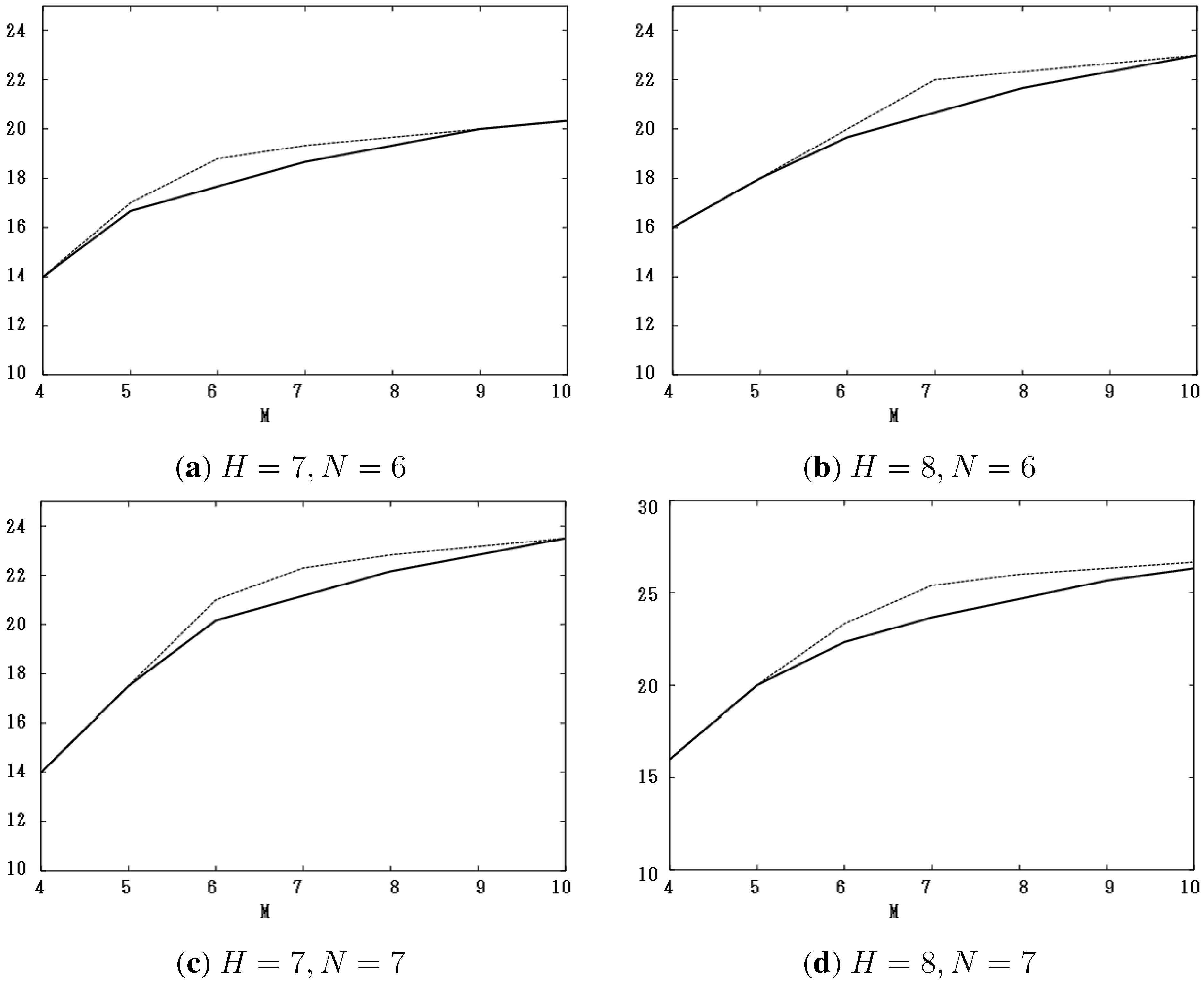
Figure 1a–d show the values of new bounds, , for (a) , (b) , (c) and (d) with , respectively. We compare these values with those obtained by the past work in [14]. In the figures, the horizontal axis is the number, M, and the vertical one, the value of such bounds. The dashed lines indicate the bounds obtained by the past work. These figures show that new bounds are not greater than old ones.
Figure 1.
The values of new bounds, , for (a) ; (b) ; (c) and (d) with , compared with the bounds obtained by the past work in [14].
Figure 1.
The values of new bounds, , for (a) ; (b) ; (c) and (d) with , compared with the bounds obtained by the past work in [14].

In paper [24], we had exact values for :
where: and we had:
We had other exact values when H is small on paper [14]. Both sets of exact values are the bounded values in Theorem 5.
3.1. A Learning Coefficient for a Three-Layered Neural Network
3.2. A Learning Coefficient for a Normal Mixture Model
Consider normal mixture models with H peaks and the true distribution with r peaks. Then, their learning coefficients, λ, are as follows [14,18]:
In particular, we have for :
where .
4. Conclusions
In this paper, we prove two theorems, Theorem 2 (the method for finding a deepest singular point) and Theorem 3 (the method to add variables) for obtaining learning coefficients in a homogeneous case. By applying these methods to Vandermonde matrix-type singularities and using the inclusion of ideals and recursive blowup from algebraic geometry, we found new bounds on learning coefficients for Vandermonde matrix-type singularities. These bounds are much tighter than those in [14]. Our future research aim is to improve our methods and to obtain exact values for the general machine model.
The learning coefficients from our recent results have been used very effectively by Drton [25,26] for model selection, using a method called “singular Bayesian information criterion (sBIC)”, which can be applied to singular models, where the assumptions supporting the use of the standard BIC do not hold. Our theoretical results introduce a mathematical measure of precision to numerical calculations, such as Markov chain Monte Carlo (MCMC). Nagata and Watanabe [27,28] gave a mathematical foundation for analyzing and developing the precision of the MCMC method using our theoretical values of marginal likelihoods.
Acknowledgments
This research was supported by the Ministry of Education, Culture, Sports, Science and Technology in Japan, Grant-in-Aid for Scientific Research 22540224.
Conflicts of Interest
The authors declare no conflict of interest.
Appendix A
We introduce Hironaka’s Theorem on desingularization.
Theorem 6
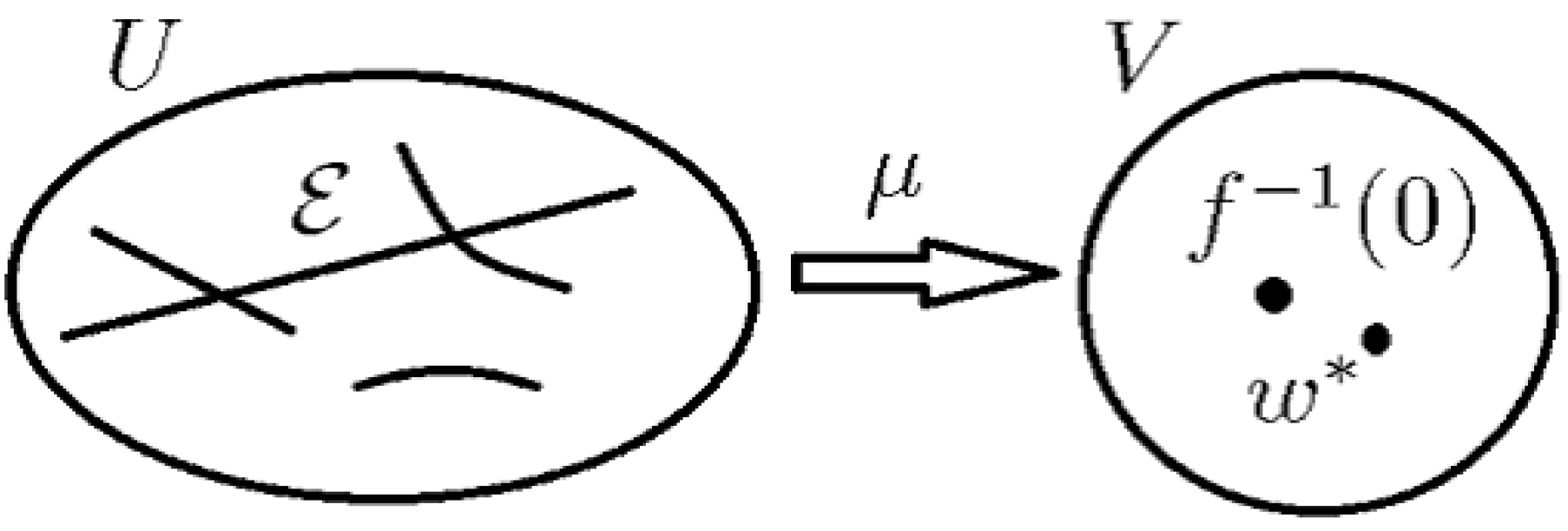
[Desingularization, Hironaka (1964), (Figure A1)]
Let f be a real analytic function in a neighborhood of with . There exists an open set, , a real analytic manifold, U, and a proper analytic map, μ, from U to V, such that:
- (1)
- is an isomorphism, where ,
- (2)
- for each , there is a local analytic coordinate system , such that , where are non-negative integers.
Figure A1.
Hironaka’s Theorem: diagram of desingularization, μ, of f: maps to . is isomorphic to by μ, where V is a small neighborhood of with .
Figure A1.
Hironaka’s Theorem: diagram of desingularization, μ, of f: maps to . is isomorphic to by μ, where V is a small neighborhood of with .

Appendix B
The learning coefficient is the log canonical threshold of the Kullback function (relative entropy). In this section, we explain its difference for real and complex fields. Let f be a nonzero holomorphic function over or an analytic function over on a smooth variety, Y, and let be a closed subscheme. The log canonical threshold, , is defined analytically as:
over , and:
over [11,12]. It is known that if f is a polynomial or a convergent power series, then is the largest root of the Bernstein-Sato polynomial, , of f, where for a linear differential operator, P [29,30,31]. The log canonical threshold, , also corresponds to the largest pole of over , ( over ), where is a function with a compact support, such that on Z.
Appendix C
Using the blowup process and the method to add variables together with the inductive method for s, we demonstrate Theorem 5
We give below Lemma 1, as it is frequently used in the proofs.
The following lemma is also used in the proofs.
Lemma 2
Step 1
Let us consider the following procedure from to , and the generators of the ideal:
By constructing the blowup repeatedly and choosing one branch of the blowup process, we show the following (i)∼(v) in this subsection:
- (i)
- ,
- (ii)
- for ,
- (iii)
- and ,
- (iv)
- The Jacobian is:and
- (v)
By Theorem 3, we can set as a variable.
Now, we show the above by the inductive method.
Define . Construct the blowup along . Set for and set .
By constructing the blowup along repeatedly, and by choosing one branch of the blowup process, set for , where .
Consider a sufficiently small neighborhood of using Theorem 2.
Set for , and for .
We then have:
which is an element of the vector ideal:
Furthermore, we have: is an element of:
Since for , where , we have and is finite. That is, we have:
If we assume that for α:
we have for :
since for , we have:
Therefore, by setting:
for and by setting again, we have:
with (i)∼(iv).
Step 2
By Step 1, we need to consider the ideal:
with Jacobian:
where:
We have:
where:
Set Then, we have:
By the above equation, we have bound. By [19], we have bound and bound, thus completing the proof.
References
- Hartigan, J.A. A Failure of Likelihood Ratio Asymptotics for Normal Mixtures. In Proceedings of the Berkeley Conference in Honor of J.Neyman and J.Kiefer, California, CA, USA, 1985; Volume 2, pp. 807–810.
- Sussmann, H.J. Uniqueness of the weights for minimal feed-forward nets with a given input-output map. Neural Netw. 1992, 5, 589–593. [Google Scholar] [CrossRef]
- Hagiwara, K.; Toda, N.; Usui, S. On the problem of applying AIC to determine the structure of a layered feed-forward neural network. In Proceedings of the IJCNN Nagoya Japan, Nagoya Congress Center, Japan, 25–29 October 1993; Volume 3, pp. 2263–2266.
- Fukumizu, K. A regularity condition of the information matrix of a multilayer perceptron network. Neural Netw. 1996, 9, 871–879. [Google Scholar] [CrossRef]
- Akaike, H. A new look at the statistical model identification. IEEE Trans. Autom. Control 1974, 19, 716–723. [Google Scholar] [CrossRef]
- Watanabe, S. Algebraic analysis for nonidentifiable learning machines. Neural Comput. 2001, 13, 899–933. [Google Scholar] [CrossRef] [PubMed]
- Watanabe, S. Algebraic geometrical methods for hierarchical learning machines. Neural Netw. 2001, 14, 1049–1060. [Google Scholar] [CrossRef]
- Watanabe, S. Algebraic geometry of learning machines with singularities and their prior distributions. J. Jpn. Soc. Artif. Intell. 2001, 16, 308–315. [Google Scholar]
- Watanabe, S. Algebraic Geometry and Statistical Learning Theory; Cambridge University Press: New York, NY, USA, 2009; Volume 25. [Google Scholar]
- Fulton, W. Introduction to Toric Varieties, Annals of Mathematics Studies; Princeton University Press: Princeton, NJ, USA, 1993. [Google Scholar]
- Kollár, J. Singularities of Pairs. In Algebraic Geometry-Santa Cruz 1995, Series Proceedings of Symposia in Pure Mathematics, 9–29 July 1995; American Mathematical Society: Providence, RI, USA, 1997; Volume 62, pp. 221–287. [Google Scholar]
- Mustata, M. Singularities of pairs via jet schemes. J. Am. Math. Soc. 2002, 15, 599–615. [Google Scholar] [CrossRef]
- Yamazaki, K.; Aoyagi, M.; Watanabe, S. Asymptotic analysis of Bayesian generalization error with Newton diagram. Neural Netw. 2010, 23, 35–43. [Google Scholar] [CrossRef] [PubMed]
- Aoyagi, M.; Nagata, K. Learning coefficient of generalization error in Bayesian estimation and Vandermonde matrix type singularity. Neural Comput. 2012, 24, 1569–1610. [Google Scholar] [CrossRef] [PubMed]
- Aoyagi, M.; Watanabe, S. Stochastic complexities of reduced rank regression in Bayesian estimation. Neural Netw. 2005, 18, 924–933. [Google Scholar] [CrossRef] [PubMed]
- Aoyagi, M.; Watanabe, S. Resolution of singularities and the generalization error with Bayesian estimation for layered neural network. IEICE Trans. J88-D-II 2005, 10, 2112–2124. [Google Scholar]
- Aoyagi, M. The zeta function of learning theory and generalization error of three layered neural perceptron. RIMS Kokyuroku Recent Top. Real Complex Singul. 2006, 1501, 153–167. [Google Scholar]
- Aoyagi, M. A Bayesian learning coefficient of generalization error and Vandermonde matrix-type singularities. Commun. Stat. Theory Methods 2010, 39, 2667–2687. [Google Scholar] [CrossRef]
- Aoyagi, M. Learning coefficient in Bayesian estimation of restricted Boltzmann machine. J. Algebr. Stat. 2013, in press. [Google Scholar] [CrossRef]
- Rusakov, D.; Geiger, D. Asymptotic Model Selection for Naive Bayesian Networks. In Proceedings of the Eighteenth Conference on Uncertainty in Artificial Intelligence, Alberta, Canada, 1–4 August 2002; pp. 438–445.
- Rusakov, D.; Geiger, D. Asymptotic model selection for naive Bayesian networks. J. Mach. Learn. Res. 2005, 6, 1–35. [Google Scholar]
- Zwiernik, P. An asymptotic behavior of the marginal likelihood for general Markov models. J. Mach. Learn. Res. 2011, 12, 3283–3310. [Google Scholar]
- Watanabe, S. Equations of states in singular statistical estimation. Neural Netw. 2010, 23, 20–34. [Google Scholar] [CrossRef] [PubMed]
- Aoyagi, M. Log canonical threshold of Vandermonde matrix type singularities and generalization error of a three layered neural network. Int. J. Pure Appl. Math. 2009, 52, 177–204. [Google Scholar]
- Drton, M. Conference Lecture: Reduced Rank Regression. Workshop on Singular Learning Theory, AIM 2011. Available online: http://math.berkeley.edu/critch/slt2011/ (accessed on 16 December 2011).
- Drton, M. Conference Lecture: Bayesian Information Criterion for Singular Models. Algebraic Statistics 2012 in the Alleghenies at The Pennsylvania State University. Available online: http://jasonmorton.com/aspsu2012/ (accessed on 15 June 2012).
- Nagata, K.; Watanabe, S. Exchange Monte Carlo Sampling from Bayesian posterior for singular learning machines. IEEE Trans. Neural Netw. 2008, 19, 1253–1266. [Google Scholar] [CrossRef]
- Nagata, K.; Watanabe, S. Asymptotic behavior of exchange ratio in exchange Monte Carlo method. Int. J. Neural Netw. 2008, 21, 980–988. [Google Scholar] [CrossRef] [PubMed]
- Bernstein, I.N. The analytic continuation of generalized functions with respect to a parameter. Funct. Anal. Appl. 1972, 6, 26–40. [Google Scholar]
- Bjőrk, J.E. Rings of Differential Operators; North-Holland: Amsterdam, The Netherlands, 1979. [Google Scholar]
- Kashiwara, M. B-functions and holonomic systems. Invent. Math. 1976, 38, 33–53. [Google Scholar] [CrossRef]
- Lin, S. Asymptotic approximation of marginal likelihood integrals. 2010; arXiv:1003.5338v2. [Google Scholar]
© 2013 by the author; licensee MDPI, Basel, Switzerland. This article is an open access article distributed under the terms and conditions of the Creative Commons Attribution license (http://creativecommons.org/licenses/by/3.0/).
Share and Cite
MDPI and ACS Style
Aoyagi, M. Consideration on Singularities in Learning Theory and the Learning Coefficient. Entropy 2013, 15, 3714-3733. https://doi.org/10.3390/e15093714
AMA Style
Aoyagi M. Consideration on Singularities in Learning Theory and the Learning Coefficient. Entropy. 2013; 15(9):3714-3733. https://doi.org/10.3390/e15093714
Chicago/Turabian StyleAoyagi, Miki. 2013. "Consideration on Singularities in Learning Theory and the Learning Coefficient" Entropy 15, no. 9: 3714-3733. https://doi.org/10.3390/e15093714