On the Calculation of Solid-Fluid Contact Angles from Molecular Dynamics

Abstract
:
1. Introduction


2. Methodology
2.1. Identification of Interfacial Molecules
- (1)
- We divide the simulation box into subcells, and calculate the local number density in each subcell.
- (2)
- We mark subcells as liquid if their number density is greater than a cutoff value ρc, otherwise we mark them as vapor cells. The cutoff density is chosen close to the average between the liquid and vapor number densities at the conditions of interest.
- (3)
- Every subcell that is adjacent to at least one liquid cell and one vapor cell is marked as an interface cell.
- (4)
- Finally, all molecules contained within the above-determined interface cells are marked as interfacial molecules.

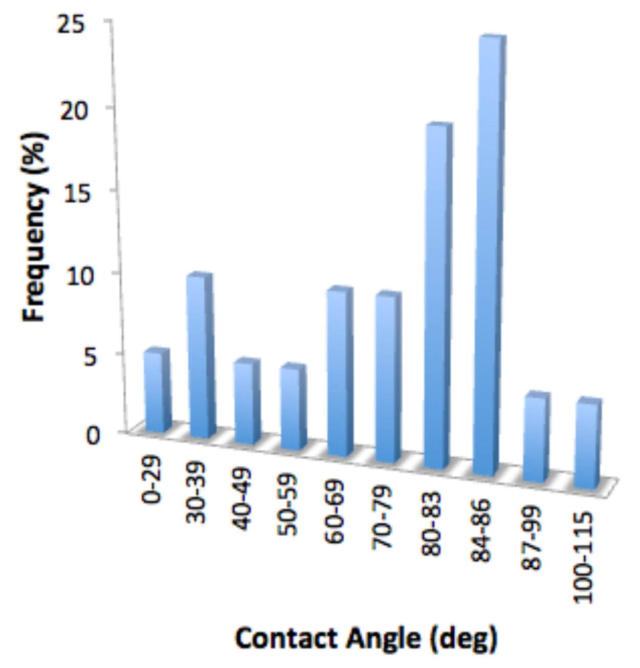
2.2. Estimation of Local Contact Angles
- (a)
- Find all the interface molecules within a given cutoff radius, rc, of molecule i.
- (b)
- Find the average position ravg of all the interface molecules found in step (a), including molecule i.
- (c)
- Subtract the average position from the position of all the neighboring molecules, including i.
- (d)
- Construct the covariance matrix of the centered positions, found in step (c):where
![Entropy 15 03734 i001]()
![Entropy 15 03734 i002]() denotes the outer (Kronecker) product.
denotes the outer (Kronecker) product. - (e)
- Find the eigenvector of Ω corresponding to its smallest eigenvalue. This is the normal to the plane that best fits the set of molecules in step (c). The sign of this normal is chosen to point away from the center of the droplet [20].


2.3. Molecular Dynamics Details

| Interaction | σ [nm] | ε/kB [K] | λr, λa | C ×102 [kJ mol−1 nmλa] | A × 104 [kJ mol−1 nmλr] |
|---|---|---|---|---|---|
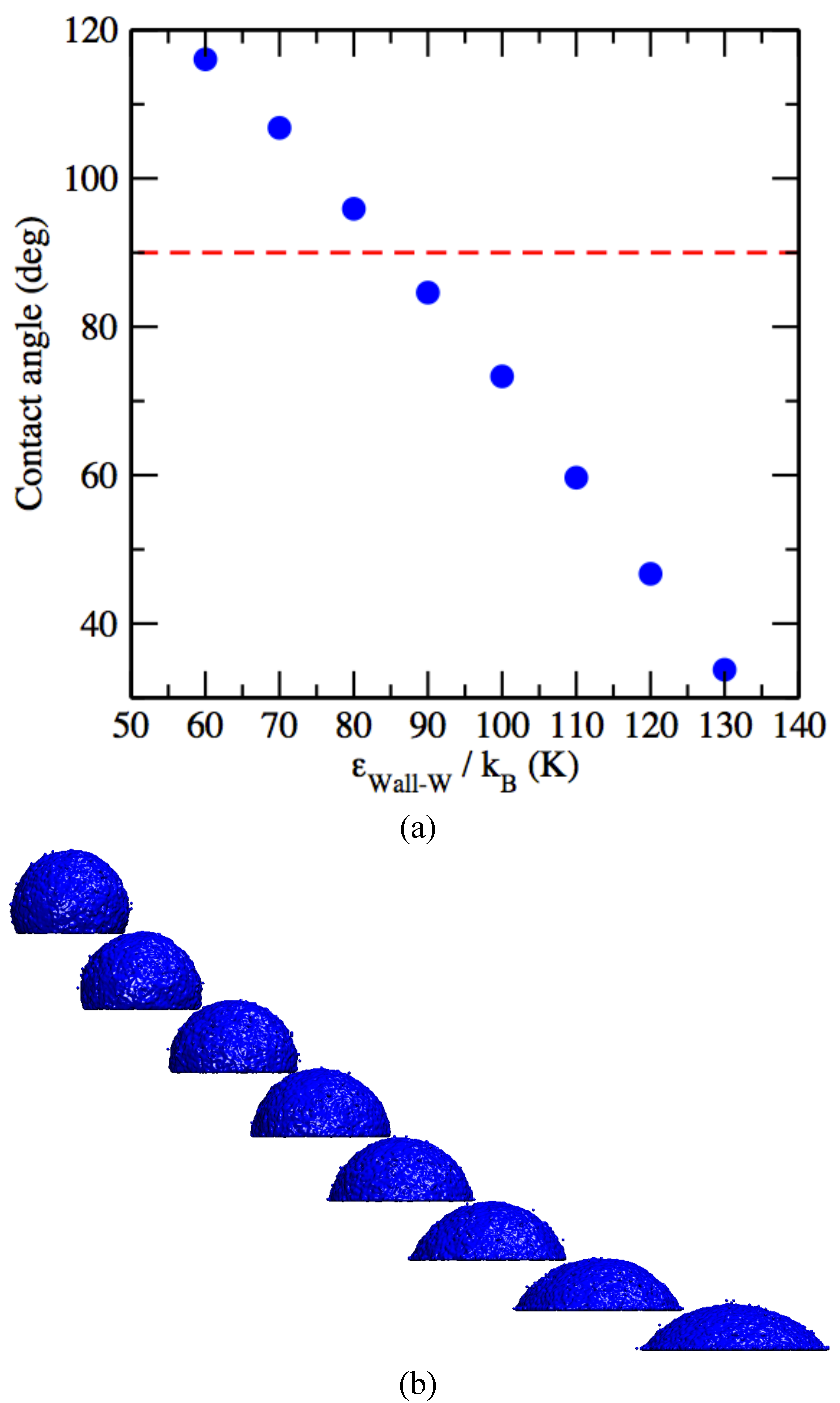
| εWall01-W/kB | 0.38716 | 60 | 10, 4 | 3.44107 | 1.15888 |
| εWall02-W/kB | 70 | 4.01458 | 1.35203 | ||
| εWall03-W/kB | 80 | 4.58810 | 1.54518 | ||
| εWall04-W/kB | 90 | 5.16161 | 1.73832 | ||
| εWall05-W/kB | 100 | 5.73512 | 1.93147 | ||
| εWall06-W/kB | 110 | 6.30863 | 2.12462 | ||
| εWall07-W/kB | 120 | 6.88214 | 2.31776 | ||
| εWall08-W/kB | 130 | 7.45565 | 2.51091 | ||
| εW-W/kB | 0.37459 | 399.96 | 8, 6 | 8.71139 | 1.222380 × 10² |
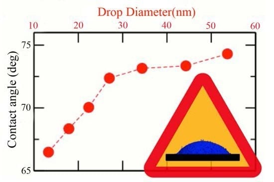
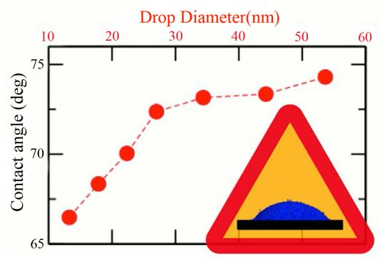
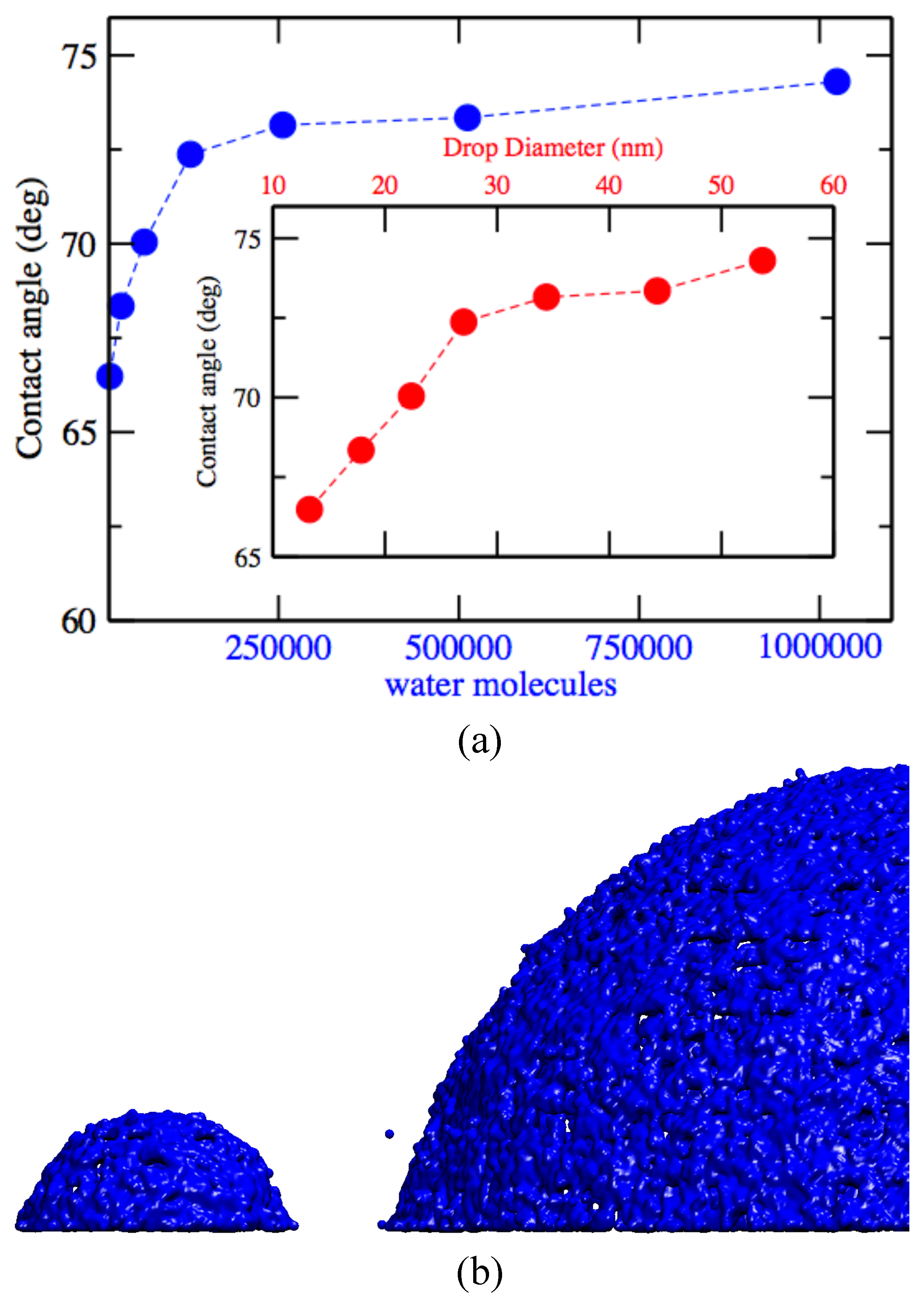
3. Results and Discussions
| Water molecules | xy-dimensions [nm] | z-dimension [nm] |
|---|---|---|
| 16,000 | 60 × 60 | 18 |
| 32,000 | ||
| 64,000 | ||
| 128,000 | ||
| 256,000 | 80 × 80 | 37.2 |
| 512,000 | ||
| 1,024,000 | 144 × 144 | 48 |


4. Conclusions
Supplementary Materials
Supplementary File 1Acknowledgments
Conflicts of Interest
References
- Mattia, D. Templated growth and characterization of carbon nanotubes for nanofluidic applications. Ph.D. Thesis, Drexel University, Philadelphia, PA, USA, 2007. [Google Scholar]
- Werder, T.; Walther, J.H.; Jaffe, R.L.; Halicioglu, T.; Koumoutsakos, P. On the water−carbon interaction for use in molecular dynamics simulations of graphite and carbon nanotubes. J. Phys. Chem. B 2003, 107, 1345–1352. [Google Scholar] [CrossRef]
- Fowkes, F.M.; Harkins, W.D. The state of monolayers adsorbed at the interface solid-aqueous solution. J. Am. Chem. Soc. 1940, 62, 3377–3386. [Google Scholar] [CrossRef]
- Schrader, M.E. Ultrahigh-vacuum techniques in the measurement of contact angles. LEED study of the effect of structure on the wettability of graphite. J. Phys. Chem. 1980, 84, 2774–2779. [Google Scholar] [CrossRef]
- Hirvi, J.T.; Pakkanee, T.A. Molecular dynamics simulations of water droplets on polymer surfaces. J. Chem. Phys. 2006, 125, 144712. [Google Scholar] [CrossRef] [PubMed]
- Hirvi, J.T.; Pakkanee, T.A. Enhanced hydrophobicity of rough polymer surfaces. J. Phys. Chem. B 2007, 111, 3336–3341. [Google Scholar] [CrossRef] [PubMed]
- Hirvi, J.T.; Pakkanee, T.A. Wetting of nanogrooved polymer surfaces. Langmuir 2007, 23, 7724–7729. [Google Scholar] [CrossRef] [PubMed]
- Ponter, A.B.; Yekta-Fard, M. The influence of environment on the drop size-contact angle relationship. Colloid Polym. Sci. 1985, 263, 673–681. [Google Scholar] [CrossRef]
- Li, H.; Zeng, X.C. Wetting and interfacial properties of water nanodroplets in contact with graphene and monolayer boron-nitride sheets. ACS NANO 2012, 6, 2401–2409. [Google Scholar] [CrossRef] [PubMed]
- Sampayo, J.G.; Malijevský, A.; Müller, E.A.; de Miguel, E.; Jackson, G. Communications: Evidence for the role of fluctuations in the thermodynamics of nanoscale drops and the implications in computations of the surface tension. J. Chem. Phys. 2010, 132, 141101. [Google Scholar] [CrossRef] [PubMed]
- Malijevský, A.; Jackson, G. A perspective on the interfacial properties of nanoscopic liquid drops. J. Phys. Cond. Matt. 2012, 24, 464121. [Google Scholar] [CrossRef] [PubMed]
- Ingebrigtsen, T.; Toxvaerd, S. Contact angles of Lennard-Jones liquids and droplets on planar surfaces. J. Phys. Chem. C 2007, 111, 8518–8523. [Google Scholar] [CrossRef]
- Shi, B.; Dhir, V.K. Molecular dynamics simulation of the contact angle of liquids on solid surfaces. J. Chem. Phys. 2009, 130, 034705. [Google Scholar] [CrossRef] [PubMed]
- De Ruijter, M.J.; Blake, T.D.; de Coninck, J. Dynamic wetting studied by molecular modeling simulations of droplet spreading. Langmuir 1999, 15, 7836–7847. [Google Scholar] [CrossRef]
- Hautman, J.; Klein, M.L. Microscopic wetting phenomena. Phys Rev. Lett. 1991, 67, 1763–1766. [Google Scholar] [CrossRef] [PubMed]
- Sergi, D.; Scocchi, G.; Ortona, A. Molecular dynamics simulations of the contact angle between water droplets and graphite surfaces. Fluid Phase Equilib. 2012, 332, 173–177. [Google Scholar] [CrossRef]
- Das, S.K.; Binder, K. Does Young’s equation hold on the nanocale? A monte Carlo test for the binary Lennard-Jones fluid. Europhys. Lett. 2006, 92, 26006. [Google Scholar] [CrossRef]
- Falconer, K. Fractal Geometry: Mathematical Foundations and Applications; Wiley: Chichester, UK, 1990. [Google Scholar]
- Mandelbrot, B. The Fractal Geometry of Nature; Macmillan: New York, NY, USA, 1983. [Google Scholar]
- Berkmann, J.; Caelli, T. Computation of surface geometry and segmentation using covariance techniques. IEEE Trans. Pattern Anal. 1994, 16, 1114–1116. [Google Scholar] [CrossRef]
- Mitra, N.J.; Nguyen, A.; Guibas, L. Estimating surface normals in noisy point cloud data. Int. J. Comput. Geom. Appl. 2004, 14, 261–276. [Google Scholar] [CrossRef]
- Efron, B.; Tibshirani, T. An Introduction to The Bootstrap; Chapman & Hall/CRC Monographs on Statistics and Applied Probability; Chapman and Hall/CRC: Boca Raton, FL, USA, 1993. [Google Scholar]
- Van der Spoel, D.; Lindahl, E.; Hess, B.; Groenhof, G.; Mark, A.E.; Berendsen, H.J. GROMACS: Fast, flexible, and free. J. Comput. Chem. 2005, 26, 1701–1718. [Google Scholar] [CrossRef] [PubMed]
- Mie, G. Zur kinetischen Theorie der einatomigen Körper. Ann. Phys. 1903, 11, 657–697. (In German) [Google Scholar] [CrossRef]
- Lobanova, O.; Avendaño, C.; Jackson, G.; Müller, E.A. SAFT-gamma force field for the simulation of molecular fluids: 5. A single-site coarse grained model of water. 2013. In preparation. [Google Scholar]
- Hadley, K.R.; McCabe, C. Coarse-grained molecular models of water: A review. Mol. Simul. 2012, 38, 671–681. [Google Scholar] [CrossRef] [PubMed]
- Avendaño, C.; Lafitte, T.; Galindo, A.; Adjiman, C.S.; Jackson, G.; Müller, E.A. SAFT-gamma force field for the simulation of molecular fluids: 1. A single-site coarse grained model of carbon dioxide. J. Phys. Chem. B 2011, 115, 11154–11169. [Google Scholar] [CrossRef] [PubMed]
- Avendaño, C.; Lafitte, T.; Adjiman, C.S.; Galindo, A.; Müller, E.A.; Jackson, G. SAFT-γ force field for the simulation of molecular fluids: 2. Coarse-grained models of greenhouse gases, refrigerants, and long alkanes. J. Phys. Chem. B 2013, 117, 2717–2733. [Google Scholar] [CrossRef] [PubMed]
- Lafitte, T.; Avendaño, C.; Papaioannou, V.; Galindo, A.; Adjiman, C.S.; Jackson, G.; Müller, E.A. SAFT-gamma force field for the simulation of molecular fluids: 3. Coarse-grained models of benzene and hetero-group models of n-decylbenzene. Mol. Phys. 2012, 110, 1189–1203. [Google Scholar] [CrossRef]
- Israelachvili, J.N. Intermolecular and Surface Forces, 3rd ed.; Elsevier: Amsterdam, The Netherlands, 2011; Chapter 11; pp. 208–211. [Google Scholar]
- Shakouri, A. EE145 Spring 2002. Available online: http://classes.soe.ucsc.edu/ee145/Spring02/EE145hmwk1Sol.pdf (accessed on 10 July 2013).
- Scocchi, G.; Sergi, D.; D’Angelo, C.; Ortona, A. Wetting and contact-line effects for spherical and cylindrical droplets on graphene layers: A comparative molecular-dynamics investigation. Phys. Rev. E 2011, 84, 061602. [Google Scholar] [CrossRef]
- Tadmor, R. Line energy, line tension and drop size. Surf. Sci. Lett. 2008, 602, L108–L111. [Google Scholar] [CrossRef]
- Weijs, J.H.; Marchand, A.; Andreotti, B.; Lohse, D.; Snoeijer, J.H. Origin of line tension for a Lennard-Jones nanodroplet. Phys. Fluids 2011, 23, 022001. [Google Scholar] [CrossRef]
- Pompe, T.; Herminghaus, S. Three-phase contact line energies from nanosclae surface topographies. Phys. Rev. Lett. 2000, 85, 1930–1933. [Google Scholar] [CrossRef] [PubMed]
- Ritchie, J.A.; Yazdi, J.S.; Bratko, D.; Luzar, A. Metastable sessile nanodroplets on nanopatterned surfaces. J. Phys. Chem. C 2012, 116, 8634–8641. [Google Scholar] [CrossRef]
- Daub, C.D.; Bartko, D.; Luzar, A. Electric control of wetting by salty nanodrops: Molecular dynamics simulations. J. Phys. Chem. C 2011, 115, 22393–22399. [Google Scholar] [CrossRef]
© 2013 by the authors; licensee MDPI, Basel, Switzerland. This article is an open access article distributed under the terms and conditions of the Creative Commons Attribution license (http://creativecommons.org/licenses/by/3.0/).
Share and Cite
Santiso, E.E.; Herdes, C.; Müller, E.A. On the Calculation of Solid-Fluid Contact Angles from Molecular Dynamics. Entropy 2013, 15, 3734-3745. https://doi.org/10.3390/e15093734
Santiso EE, Herdes C, Müller EA. On the Calculation of Solid-Fluid Contact Angles from Molecular Dynamics. Entropy. 2013; 15(9):3734-3745. https://doi.org/10.3390/e15093734
Chicago/Turabian StyleSantiso, Erik E., Carmelo Herdes, and Erich A. Müller. 2013. "On the Calculation of Solid-Fluid Contact Angles from Molecular Dynamics" Entropy 15, no. 9: 3734-3745. https://doi.org/10.3390/e15093734