1. Introduction
Since Fowler
et al. [
1], introduced a complex Lorenz model to generalize the real Lorenz model in 1982, complex chaotic and hyperchaotic systems have attracted increasing attention, due to the fact that systems with complex variables can be used to describe the physics of a detuned laser, rotating fluids, disk dynamos, electronic circuits and particle beam dynamics in high energy accelerators [
2]. When applying complex systems in communications, the complex variables will double the number of variables and can increase the content and security of the transmitted information. Many complex chaotic and hyperchaotic systems have been proposed ever since the 1980s. In [
3], the authors studied the chaotic unstable limit cycles of complex Van der Pol oscillators. The rich dynamics behaviors of the complex Chen and complex Lü systems were investigated in [
4]. By adding state feedback controllers to their complex chaotic systems, complex hyperchaotic Chen, Lorenz and Lü systems were introduced and studied in [
5,
6,
7], respectively. The authors [
8] constructed a complex nonlinear hyperchaotic system by adding a cross-product nonlinear term to the complex Lorenz system. A complex modified hyperchaotic Lü system [
9] was proposed by introducing complex variables to its real counterpart.
In 1990 [
10], Pecora and Carroll proposed the drive-response concept for constructing the synchronization of coupled chaotic systems. Over the last two decades, synchronization in chaotic systems has been extensively investigated, due to its potential applications in various fields, such as chemical reactions, biological systems and secure communication. Mahmoud
et al. [
11] designed an adaptive control scheme to study the complete synchronization of chaotic complex nonlinear systems with uncertain parameters. The authors achieved phase synchronization and antiphase synchronization of two identical hyperchaotic complex nonlinear systems via an active control technique in [
12]. Based on passive theory, the authors studied the projective synchronization of hyperchaotic complex nonlinear systems and its application in secure communications [
13]. Liu
et al. [
14] investigated the modified function projective synchronization of general chaotic complex systems described by a unified mathematical expression.
The aforementioned synchronization schemes are based on the usual drive-response synchronization mode, which has one drive system and one response system. Recently, Luo [
15] proposed a combination synchronization scheme, which has two drive systems and one response system. This synchronization scheme has advantages over the usual drive-response synchronization, such as being able to provide greater security in secure communication. In secure communication, the transmitted signals can be split into several parts, each part loaded in different drive systems, or can divide time into different intervals, the signals in different intervals being loaded in different drive systems. Thus, the transmitted signals can have stronger anti-attack ability and anti-translated capability than those transmitted by the usual transmission model.
Motivated by the above discussions, this paper aims to study the combination synchronization of three identical or different nonlinear complex hyperchaotic systems. The rest of this paper is organized as follows.
Section 2 introduces the scheme of combination synchronization. In
Section 3 and
Section 4, we investigate combination synchronization among three identical and different complex nonlinear hyperchaotic systems, respectively. Finally, conclusions are given in
Section 5.
3. Combination Synchronization among Identical Nonlinear Complex Hyperchaotic Systems
In this section, we take the complex hyperchaotic Lorenz system [
6] as an example to investigate the combination synchronization among three identical systems.
The first drive system is given by:
and the second drive system is described as follows:
The response system takes the following form:
where
α,
β,
γ and
σ are positive parameters,
are complex variables and
;
,
are real variables. The overbar represents a complex conjugate function.
and
are real controllers to be determined.
For the convenience of our discussions, we assume in our synchronization scheme.
We define error states between systems (5), (6) and (7) as:
such that:
Thus, we have the following error dynamical system:
Substituting Equations (5)–(7) in Equation (10) and separating the real and imaginary parts yields:
Then, we obtain the following results.
Theorem 1. If the controllers are chosen as follows:
then driven systems (5) and (6) will achieve combination synchronization with response system (7).
Proof. Construct the following Lyapunov function:
Taking the time derivative of
V along the trajectory of error dynamical system (11) yields:
Substituting Equation (12) into Equation (14), then:
Since
as
, according to the Lyapunov stability theory, we know
,
i.e.,
. Therefore, drive systems (5) and (6) will achieve combination synchronization with the response system (7).
This completes the proof.
The following corollaries can be easily obtained from Theorem 1.
Corollary 1. (i) Suppose that
and
, and if the controllers are chosen as follows:
then drive system (6) will achieve projective synchronization with response system (7).
(ii) Suppose that
and
, and if the controllers are chosen as follows:
then drive system (5) will achieve projective synchronization with response system (7).
Corollary 2. Suppose that
and
, and if the controllers are chosen as follows:
then system (7) is stabilized to the equilibrium,
.
Remark 1: The proofs of Corollary 1 and Corollary 2 are similar to those of theorem 1, so we omitted them.
In the following, numerical experiments are given to demonstrate our results. The fourth-order Runge-Kutta method is used with a time step size of 0.001. The system parameters are given as
and
, so that the complex Lorenz system exhibits hyperchaotic behavior. We assume
,
and
, and the initial states for drive systems (5) and (6) and response system (7) are arbitrarily given by
and
,
i.e.,
,
and
, respectively. The corresponding numerical results are shown in
Figure 1 and
Figure 2.
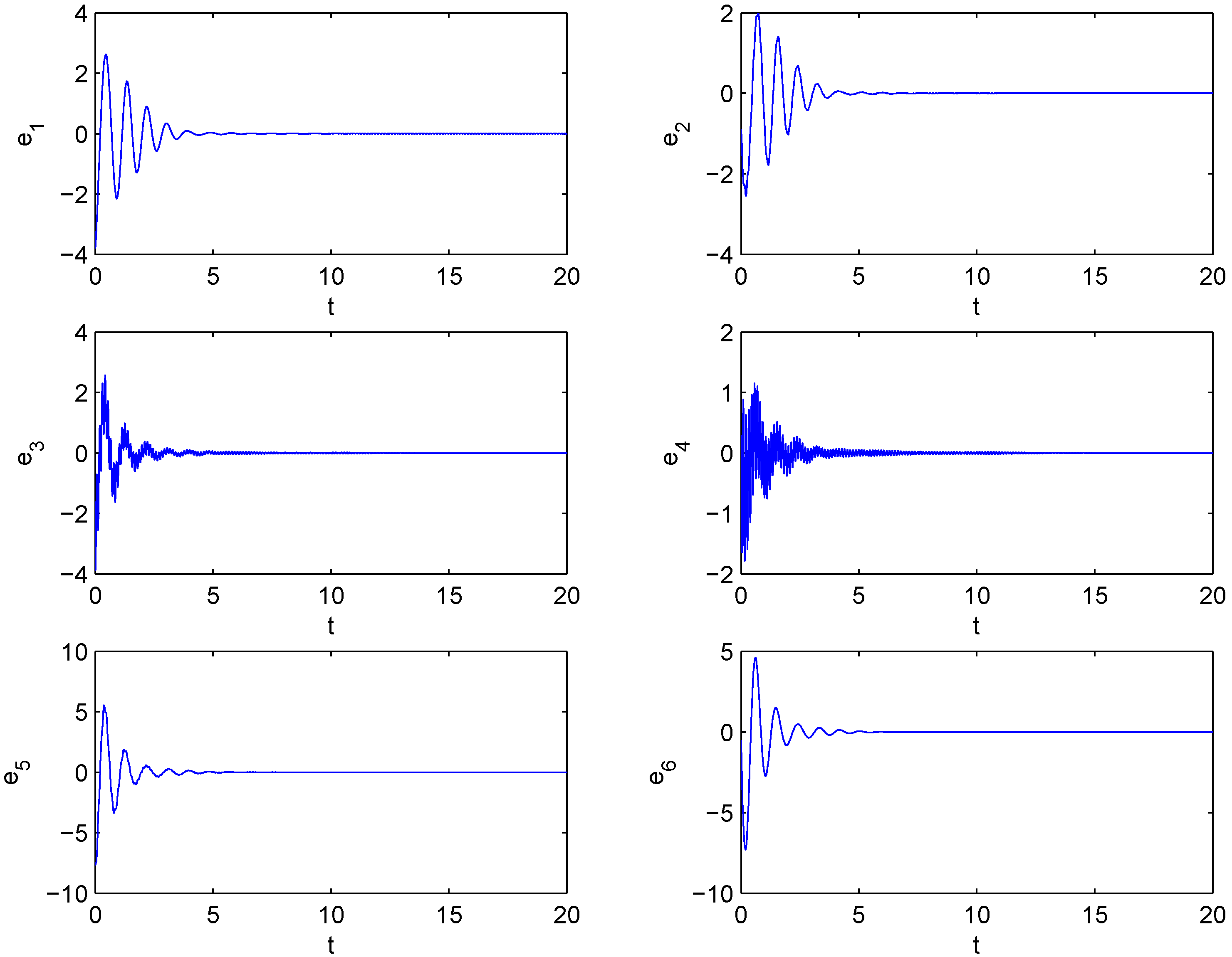
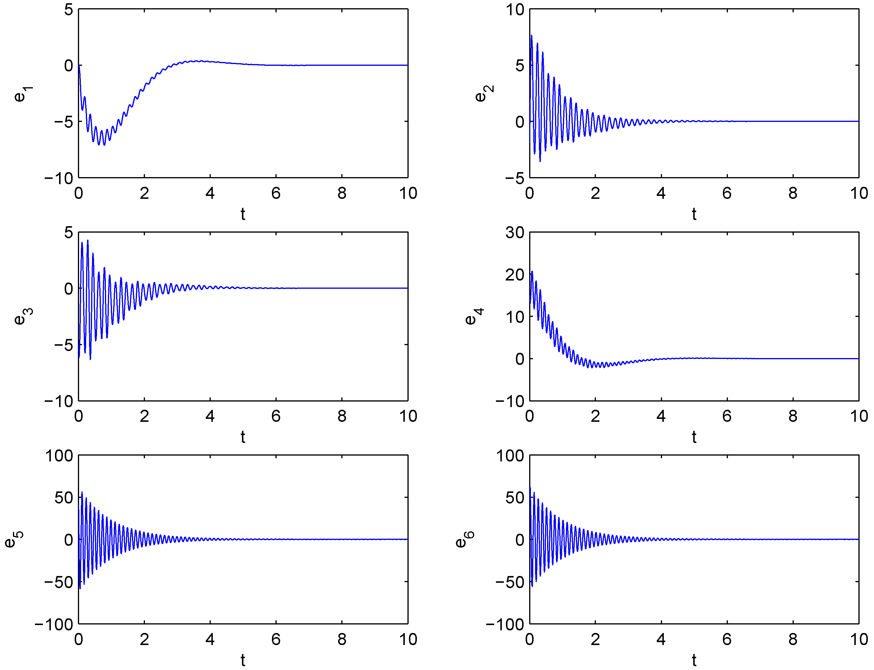
Figure 1 displays the time response of the combination synchronization errors,
. The errors converge to zero, which implies that systems (5), (6) and (7) have achieved combination synchronization.
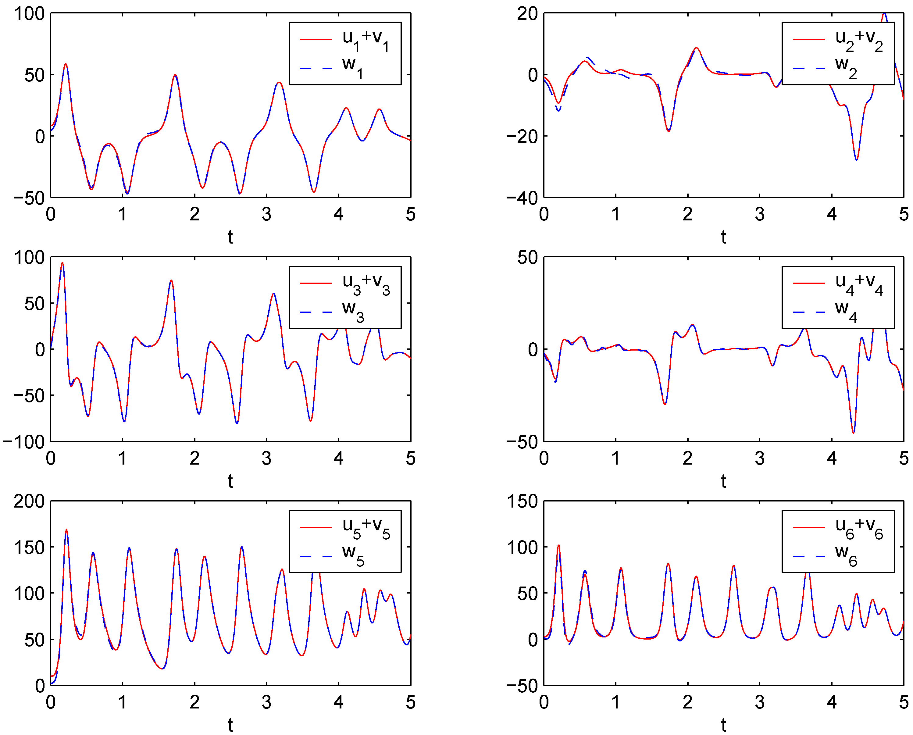
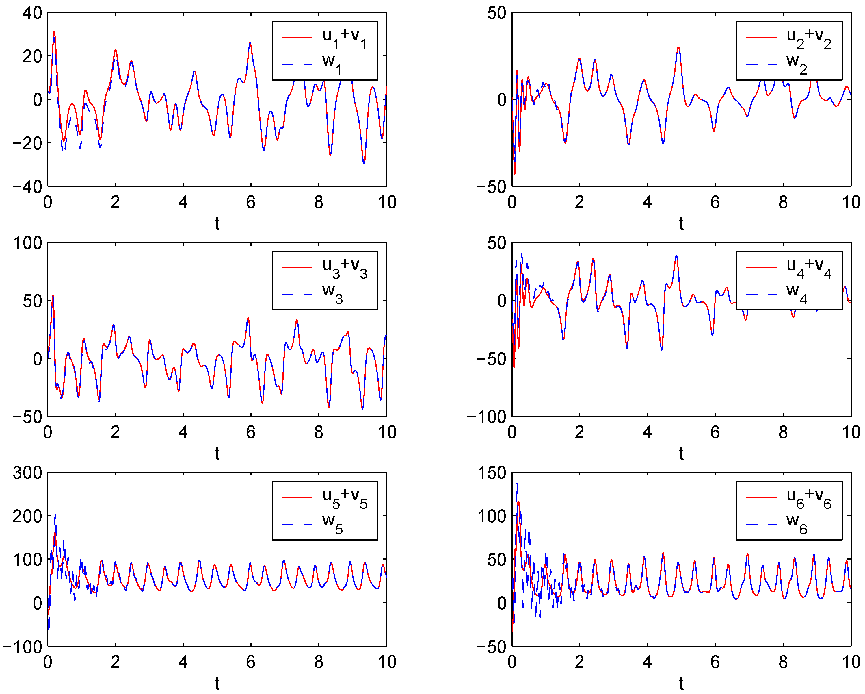
Figure 2 depicts the time responses of the states,
versus ,
versus ,
versus ,
versus ,
versus and
versus , respectively. Next, suppose that
,
and
. The time evolution of the states,
, of system (7) with controller (18) are displayed in
Figure 3, which illustrates that system (7) is stabilized to the equilibrium,
.
Figure 1.
Combination synchronization errors, , , , , and , between drive systems (5) and (6) and response system (7).
Figure 1.
Combination synchronization errors, , , , , and , between drive systems (5) and (6) and response system (7).
4. Combination Synchronization among Different Nonlinear Complex Hyperchaotic Systems
In this section, we investigate the combination synchronization among three different nonlinear complex hyperchaotic systems. The hyperchaotic complex Lorenz system [
6] and the hyperchaotic complex Chen system [
5], respectively, describe the drive systems:
and
and the hyperchaotic complex Lü system system [
7] is the response system given by:
where
,
,
,
,
,
,
,
,
,
,
and
are positive parameters,
are complex variables and
;
,
and
are real variables. The overbar represents the complex conjugate function.
and
are real control functions to be determined.
Figure 2.
Time responses for states versus , respectively.
Figure 2.
Time responses for states versus , respectively.
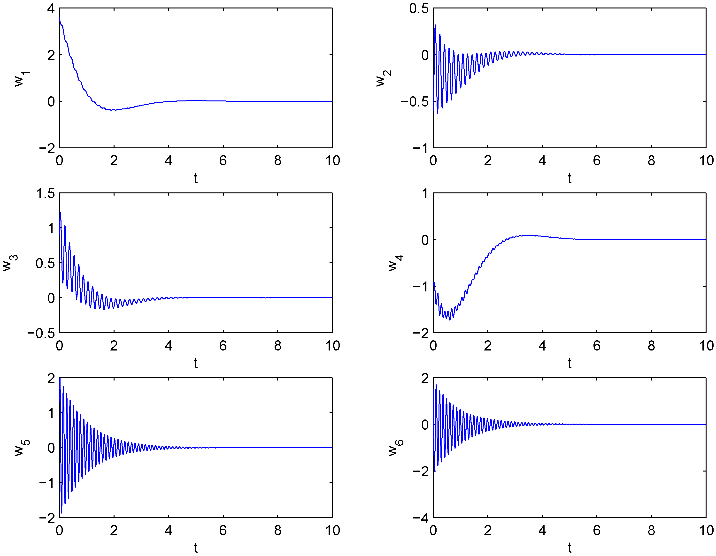
Figure 3.
Time evolution of the states for system (7).
Figure 3.
Time evolution of the states for system (7).
For the convenience of the following discussions, we assume , and in our synchronization scheme.
We define error states between drive systems (19)–(20) and response system (21) as:
such that:
Separating the real and imagery parts of Equation (22) gets the following:
Thus, we have the following error dynamical system:
Similar to
Section 3, we have the following results.
Theorem 2. If the controllers are chosen as:
then drive systems (19) and (20) will achieve combination synchronization with response system (21).
Corollary 3. (i) Suppose that
and
, and if the controllers are chosen as follows:
then drive system (20) will achieve projective synchronization with response system (21).
(ii) Suppose that
and
, and if the controllers are chosen as follows:
then drive system (19) will achieve projective synchronization with response system (21).
Corollary 4. Suppose that
,
and
, and if the controllers are chosen as follows:
then system (21) is stabilized to the equilibrium,
.
In what follows, numerical experiments are given to demonstrate our results. The fourth-order Runge-Kutta method is used with a time step size of 0.001. The system parameters are given as , , , , and , so that the three complex nonlinear hyperchaotic systems exhibit hyperchaotic behaviors, respectively.
Figure 4.
Combination synchronization errors, , , , , and , between drive systems (19), (20) and response system (21).
Figure 4.
Combination synchronization errors, , , , , and , between drive systems (19), (20) and response system (21).
First, we assume
,
and
, and the initial states for the drive systems and response systems are arbitrarily given by
and
,
i.e.,
,
and
, respectively. The corresponding numerical results are shown in
Figure 4 and
Figure 5.
Figure 4 displays the time response of the combination synchronization errors,
. The errors converge to zero, which implies that systems (19), (20) and (21) have achieved combination synchronization.
Figure 5 depicts the time responses of the states,
versus ,
versus ,
versus ,
versus ,
versus and
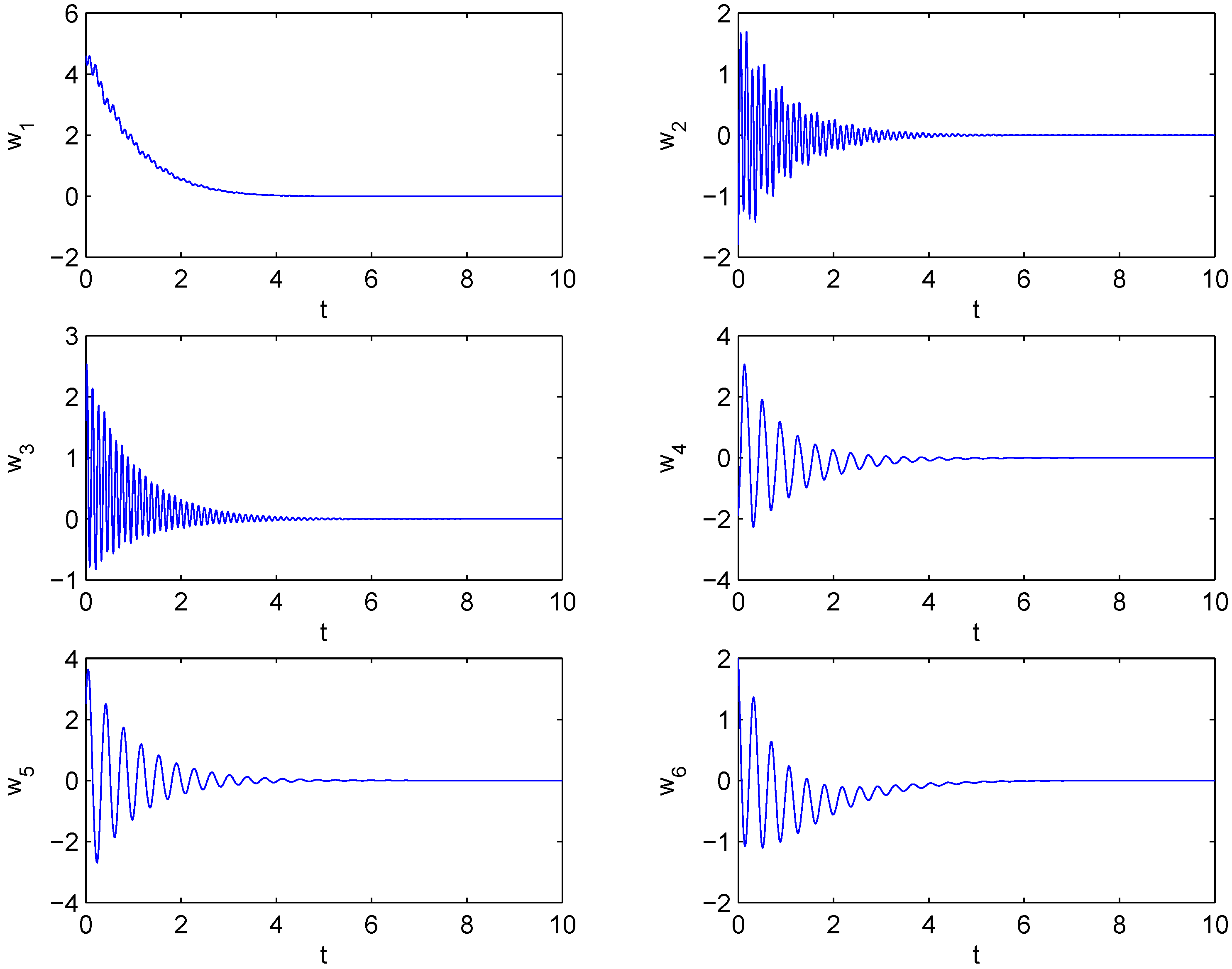
versus , respectively. When
,
and
, the time evolution of the states,
, of system (21) with controller (29) are displayed in
Figure 6, which means that system (21) is stabilized to the equilibrium,
.
Figure 5.
Time responses for states versus , respectively.
Figure 5.
Time responses for states versus , respectively.
Figure 6.
Time evolution of the states for system (21).
Figure 6.
Time evolution of the states for system (21).
