Cross-Scale Interactions and Information Transfer

Department of Nonlinear Dynamics and Complex Systems, Institute of Computer Science, Academy of Sciences of the Czech Republic, Pod vodárenskou veží 2, 182 07 Prague 8, Czech
Entropy 2014, 16(10), 5263-5289; https://doi.org/10.3390/e16105263
Submission received: 22 July 2014
/
Revised: 27 August 2014
/
Accepted: 30 September 2014
/
Published: 10 October 2014
(This article belongs to the Special Issue Information in Dynamical Systems and Complex Systems)
Abstract
:An information-theoretic approach for detecting interactions and information transfer between two systems is extended to interactions between dynamical phenomena evolving on different time scales of a complex, multiscale process. The approach is demonstrated in the detection of an information transfer from larger to smaller time scales in a model multifractal process and applied in a study of cross-scale interactions in atmospheric dynamics. Applying a form of the conditional mutual information and a statistical test based on the Fourier transform and multifractal surrogate data to about a century long records of daily mean surface air temperature from various European locations, an information transfer from larger to smaller time scales has been observed as the influence of the phase of slow oscillatory phenomena with the periods around 6–11 years on the amplitudes of the variability characterized by the smaller temporal scales from a few months to 4–5 years. These directed cross-scale interactions have a non-negligible effect on interannual air temperature variability in a large area of Europe.
1. Introduction
Emergent phenomena in complex systems consisting of many parts usually cannot be explained by a simple linear sum or a combination of properties of system components. The complex behavior is usually the result of mutual interactions of the intertwined subsystems. Knowledge about the interactions among the system constituents can be the key to understanding complex phenomena. Among various types of interactions and dependence, synchronization [1] plays a specific role in the cooperative behavior of coupled complex systems or their components. Synchronization and related phenomena have been observed in diverse physical, biological and social systems. Examples include cardio-respiratory interactions [2,3], synchronization of neural signals on various levels of organization of brain tissues [4–7], or coherent variability in the Earth atmosphere and climate [8–13]. In such systems it is not only important to detect interactions and possible synchronized states, but also to distinguish mutual interactions from a directional coupling, i.e., to identify drive-response relationships between the systems studied. This problem is a special case of the general question of causality or causal relations between systems, processes or phenomena. For more comprehensive introduction to this topic, see [14].
The first definition of causality that could be quantified and measured computationally, yet very general, was given in 1956 by N. Wiener [15]: “For two simultaneously measured signals, if we can predict the first signal better by using the past information from the second one than by using the information without it, then we call the second signal causal to the first one.”
The introduction of the concept of causality into the experimental practice, namely into analyses of data observed in consecutive time instants, time series, is due to Clive W. J. Granger, the 2003 Nobel prize winner in economy. In his Nobel lecture [16] he recalled the inspiration by Wiener’s work and identified two components of the statement about causality:
- (1)
- The cause occurs before the effect; and
- (2)
- The cause contains information about the effect that is unique, and is in no other variable.
As Granger puts it, a consequence of these statements is that the causal variable can help to forecast the effect variable after other data has been first used [16]. This restricted sense of causality, referred to as Granger causality, GC hereafter, characterizes the extent to which a process Xt is leading another process Yt, and builds upon the notion of incremental predictability. It is said that the process Xt Granger causes another process Yt if future values of Yt can be better predicted using the past values of Xt and Yt rather than only the past values of Yt. The standard test of GC developed by Granger [17] is based on a linear regression model. A number of approaches have been developed with the aim to extend the GC concept to nonlinear systems. We will briefly review the one based on information theory [18]. We will demonstrate that an information theoretic functional, known as mutual information (MI), is a useful measure of dependence that can be used in the detection of interactions of two systems (or subsystems of a complex system) using time series that record their dynamical evolution. Then the conditional mutual information (CMI) will be used in order to detect directional interactions. Paluš et al. [5] have proposed the conditional mutual information as a tool for the generalization of the GC concept for nonlinear systems. An equivalent information-theoretic quantity called “transfer entropy” has been proposed by Schreiber [19]. Barnett et al. analytically proved the equivalence of the transfer entropy and the conditional mutual information with the GC concept in the case of Gaussian processes [20]. Therefore the causal influence of a process Xt on another process, Yt, understood in the framework of the GC concept, is also frequently interpreted as an information transfer from Xt to Yt.
Several authors [21–23] extended the concept of the transfer entropy and conditional mutual information from the bivariate case of two processes into a multivariate case of many processes. In this paper, however, we will restrict the consideration to the bivariate case and we will even focus on one process evolving on many time scales and will develop an approach for detecting interactions and information transfer between dynamics evolving on different time scales.
Considering the detection of the direction of coupling between two systems, it is worthy to note the development tailored specifically for low-dimensional dynamical systems. Arnhold et al. [24] and Quiroga et al. [25] proposed a directional statistic based on distances of points in systems’ state spaces. Paluš and Vejmelka [26] critically assessed this method and compared it to the information-theoretic approach. More recent development of the methods based on the state-space geometry is due to Chicharro and Andrzejak [27] and Sugihara et al. [28]. Evaluation of these new methodological advancements in the context of cross-scale coupling can be an inspiration for further research. Here we will focus on applications of the ideas and tools from information theory [18].
2. Overview of Methods
2.1. Measuring Dependence with Mutual Information
Consider a discrete random variable X with a set of values Ξ. The probability distribution function (PDF) for X is p(x) = Pr{X = x}, x ∈ Ξ. We denote the PDF by p(x), rather than pX(x), for convenience. Analogously, in the case of two discrete random variables X and Y with the sets of values Ξ and ϒ, respectively, their probability distribution functions will be denoted as p(x), p(y) and their joint PDF as p(x, y). The entropy H(X) of a single variable, say X, is defined as
and the joint entropy H(X, Y ) of X and Y is
The conditional entropy H(Y |X) of Y given X is
The average amount of common information, contained in the variables X and Y, is quantified by the mutual information I(X; Y ), defined as
Considering Equations (1) and (2) we have
Note that two variables X and Y are independent if and only if p(x, y) = p(x)p(y), i.e.,
The mutual information (5) is in fact an averaged value of
, i.e., it quantifies the average digression from independence of the variables X and Y and constitutes a useful measure of general statistical dependence with the following properties:
- I(X; Y ) ≥ 0,
- I(X; Y ) = 0 iff X and Y are independent.
The conditional mutual information I(X; Y |Z) of the variables X, Y given the variable Z is
For Z independent of X and Y we have
By a simple manipulation we obtain
where I(X; Y ; Z) = H(X) + H(Y ) + H(Z) − H(X, Y, Z). Thus the conditional mutual information I(X; Y |Z) characterizes the “net” dependence between X and Y without a possible influence of another variable, Z.
Consider now n discrete random variables X1, . . ., Xn with values (x1, . . . , xn) ∈ Ξ1× … ×Ξn, with PDF’s p(xi) for individual variables Xi and the joint distribution p(x1, . . . , xn). The mutual information I(X1;X2; . . . ;Xn), quantifying the common information in the n variables X1, . . ., Xn can be defined as
It is possible, however, to define mutual information functionals quantifying common information of groups of variables and also various multivariate generalizations of the conditional mutual information, see [29].
All the information theoretic functionals can be defined for continuous random variables. The sums are substituted by integrals and the PDF’s by the probability distribution densities [18,30]. Among the continuous probability distributions a special role is played by the Gaussian distribution. Let X1, . . ., Xn be an n-dimensional normally distributed random variable with a zero mean and a covariance matrix C. Then (see [29,30] and references therein)
where cii are the diagonal elements (variances) and σi are the eigenvalues of the n × n covariance matrix C.
The entropy and information are usually measured in bits if the base of the logarithms in their definitions is 2, here we use the natural logarithm and therefore the units are called nats.
2.2. Inference of Causality with the Conditional Mutual Information
Let {x(t)} and {y(t)} be time series considered as realizations of stationary and ergodic stochastic processes {X(t)} and {Y(t)}, respectively, t = 1, 2, 3, . . . . In the following we will mark x(t) as x and x(t + τ ) as xτ, and the same notation holds for the series {y(t)}.
The mutual information I(y; xτ ) measures the average amount of information contained in the process {Y } about the process {X} in its future τ time units ahead (τ -future hereafter). This measure, however, could also contain information about the τ -future of the process {X} contained in this process itself, if the processes {X} and {Y } are not independent, i.e., if I(x; y) > 0. In order to obtain the “net” information about the τ -future of the process {X} contained in the process {Y } we use the conditional mutual information I(y; xτ |x). The latter was used by Paluš et al. [5] to define the coarse-grained transinformation rate, able to detect direction of coupling of unidirectionally coupled dynamical systems.
We used the standard statistical language in which we considered the time series {x(t)} and {y(t)} as realizations of stochastic processes {X(t)} and {Y(t)}, respectively. If the processes {X(t)} and {Y(t)} are substituted by dynamical systems evolving in measurable spaces of dimensions m and n, respectively, the variables x and y in I(y; xτ |x) and I(x; yτ |y) should be considered as n-dimensional and m-dimensional vectors. In experimental practice, however, usually only one observable is recorded for each system. Therefore, instead of the original components of the vectors X⃗(t) and Y⃗(t), the time delay embedding vectors according to Takens [31] are used. Then, back in the time-series representation, we have
where η and ρ are time lags used for the embedding of the trajectories X⃗(t) and Y⃗(t), respectively. Formally, also X⃗(t + τ ) should be expanded as x(t + τ ), x(t − η + τ ), . . . , x(t − (n − 1)η + τ ), however, only information about one component x(t + τ ) in the τ -future of the system {X} is used for simplicity. The CMI characterizing the influence in the opposite direction I(X⃗(t); Y⃗(t + τ)| Y⃗(t)) is defined in full analogy. Exactly the same formulation can be used for Markov processes of finite orders m and n. Based on the idea of finite-order Markov processes, Schreiber [19] has proposed a “transfer entropy”, which is an equivalent expression for the conditional mutual information (11)—see [14,26].
Extensive numerical experiences [26] suggest that the conditional mutual information in the form
is sufficient to infer coupling direction between the systems Y⃗(t) and X⃗(t). The dimensionality of the condition must contain full information about the state of the system X⃗(t) (see Section 2.3), while single components y(t) and x(t + τ ) are able to provide information about the directional coupling between the systems Y⃗(t) and X⃗(t).
2.3. Example: Unidirectionally Coupled Rössler Systems
As an example of the detection of unidirectional coupling using the conditional mutual information, we consider the unidirectionally coupled Rössler systems, studied in detail by Paluš and Vejmelka [26], given by the equations
for the autonomous system {X}, and
for the response system {Y }. We will use the parameters a1 = a2 = 0.15, b1 = b2 = 0.2, c1 = c2 = 10.0, and frequencies ω1 = 1.015 and ω2 = 0.985, i.e., the two systems are similar, but not identical. The system {X} is autonomous, and it is the “master” that drives the system {Y } through the diffusive coupling term ε(x1 – y1) in the right hand side of the first component of the driven (“slave”) system {Y }. The parameter ε is referred to as the “coupling strength”. We generate time series as solutions of the system (13) and (14) for different coupling strengths ε and estimate the conditional mutual information in order to assess the existence of directional coupling or information transfer from the system {X} to the system {Y } and vice versa.
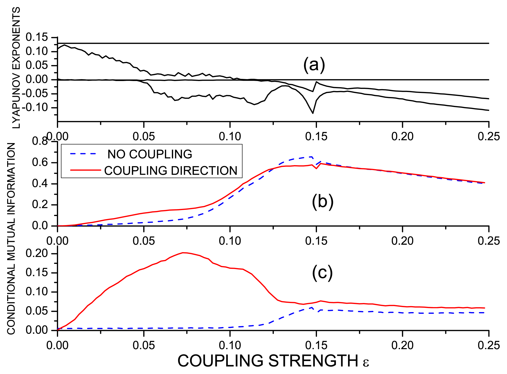
Figure 1a presents four Lyapunov exponents (LE) of the coupled systems (the two negative LE’s are not shown) as functions of the coupling strength ε. One positive and one zero LE of the driving system {X} are constant, while the LE’s of the driven system {Y }, which are positive and zero without a coupling or with a weak coupling, decrease with increasing ε. The two systems can enter a synchronized regime when the originally positive LE of the response system becomes negative [32].
Comparing LE and CMI as functions of the coupling strength ε brings a very important observation: the direction of coupling can be reliably detected when the two systems are coupled but not yet synchronized (for more details see [26]). Therefore, before inferring the directionality of coupling one should also assess a possibility of synchronization. In the following we will focus on the results for ε between 0 and approximately 0.12.
With the 1-dimensional condition, both CMI I(x(t); y(t + τ)|y(t)) and I(y(t); x(t + τ)|x(t)) (Figure 1b) are increasing with increasing ε. Some authors would interpret the inequality
as an evidence for a causal influence and existence of a positive information flow
from {X} to {Y }. Although the direction of the causal influence inferred in such a way is correct in this case, such an inference is not valid in general. Paluš and Vejmelka [26] demonstrate that estimates of CMI are biased, and if the two studied systems are not identical, the bias in the direction X → Y is different from the bias in the direction Y → X. Typically, the bias is larger in the direction from a slower to a faster system (considering main frequencies, ω1 and ω2 in our example), or from a system with simpler dynamics to a system with more complex dynamics (e.g., a periodic system seemingly drives a chaotic system). Also different noise levels can differently bias the CMI estimates. Therefore, for the correct inference of a causal influence in the sense of the unidirectional coupling, the causality measure must (asymptotically) vanish in the uncoupled direction. Using CMI (12), this requirement is met with the conditioning dimension, which allows a full description of a state of the driven system in its uncoupled state. For the Rössler system the necessary conditioning dimension is three. It is demonstrated in Figure 1c where I(y(t); x(t+τ )|x(t), x(t−η), x(t − 2η)) in the uncoupled direction stays at a zero level and begins to increase only when ε approaches the synchronization threshold and the possibility to infer the direction of coupling is lost. In the direction of coupling, I(x(t); y(t + τ )|y(t), y(t − η), y(t − 2η)) is distinctly positive from small values of ε up to the synchronization threshold. The behavior of CMI with the 3-dimensional condition (Figure 1c) is the same [26] irrespective of the way how the 3-dimensional condition is constructed—either we use the original components x1(t), x2(t), x3(t) of the system (13), or a time-delay trajectory reconstruction x1(t), x1(t − η), x1(t − 2η) according to Takens embedding theorem [31]. The time delay η is chosen as the first minimum of the auto-mutual information I(x1(t); x1(t + η)) following the Fraser–Swinney recipe [33].
2.4. Interactions over Time Scales
In previous sections we have considered inference of interactions and directed coupling in the case of two different systems (or signals/time series representing two different systems). Let us consider now just one system {X}, characterized by a time series {x(t)}. The system {X} evolves simultaneously on many time scales. How can we find whether dynamics on different time scales evolve in a mutually independent way, or there are some interactions between dynamics on different time scales?
The first step is a scale-wise decomposition of the studied dynamics/time series. Since we focus on interactions over time scales, a relevant scale-wise decomposition is a decomposition of a signal into a number of components with limited frequency bandwidths. A number of authors, e.g., Gans et al. [34] use a set of digital filters. A wavelet transform, decomposing a signal into a set of components with predefined central frequencies and spectral bandwidths [35], is also a frequently used approach. Oscillatory components whose parameters are not pre-defined but emerge from particular analyzed data can be obtained using empirical mode decomposition [36] or singular-system analysis (see [9,37] and references therein).
A (quasi)oscillatory component {sf(t)} can conveniently be decomposed into its instantaneous phase and amplitude (Figure 2) using the analytic signal approach [1].
For an arbitrary time series s(t) the analytic signal ψ(t) is a complex function of time defined as
The instantaneous phase φ(t) of the signal s(t) is then
and its instantaneous amplitude is
The imaginary part ŝ(t) of the analytic signal ψ(t) is usually obtained by using the Hilbert transform of s(t) [1,34]. Since the Hilbert transform is a unit gain filter at each frequency, broad-band signals from multiscale processes are usually pre-filtered to the frequency band of interest, as in the abovementioned approach of Gans et al. [34]. Also in the case when the empirical mode decomposition (EMD) approach is used for the scale-wise decomposition, the Hilbert transform is applied to each oscillatory mode obtained by the EMD procedure. On the other hand, singular-system analysis (SSA) provides oscillatory modes in twins shifted by π/2, which can be directly used in Equations (16) and (17) for the estimation of the phase φ(t) and the amplitude A(t), respectively [9,38]. Also a continuous complex wavelet transform (CCWT hereafter) [39] can be directly applied to an experimental time series x(t) reflecting the dynamics of a multiscale system. CCWT converts the time series x(t) into a set of complex wavelet coefficients W(t, f):
In the following we use the complex Morlet wavelet [39]:
where σt is the bandwidth parameter, and f0 is the central frequency of the wavelet. σt determines the rate of the decay of the Gauss function, and its reciprocal value σf = 1/πσt determines the spectral bandwidth. At each time scale given by the central wavelet frequency, the complex wavelet coefficients can be directly used in Equations (16) and (17) for the estimation of the phase φ(t) and the amplitude A(t), respectively. The CCWT provides both the band-pass filtering of the original multiscale signal and the estimation of the instantaneous phase and the instantaneous amplitude.
Having a multiscale signal (a time series x(t) reflecting the dynamics of a multiscale system) decomposed into a number of scale-specific (or frequency-specific) modes described using their instantaneous phases and amplitudes, it is possible to study cross-scale interactions of the following types:
- phase–phase
- amplitude–amplitude
- phase–amplitude
Some authors also compute the instantaneous frequency as a time derivative of the instantaneous phase [34,40] and assess the cross-frequency coupling between different instantaneous frequencies or combinations of the instantaneous frequency with the instantaneous phase or amplitude [40]. The instantaneous amplitude is also called an envelope (of fast oscillations) and its square is related to power, which is also evaluated in cross-frequency analysis of brain signals [40]. We can also study the cross-scale relations using directly the (filtered) signals s(t) obtained for individual scales, e.g., in the case of the CCWT decomposition defined as s(t) = Real{W(t, f)}. The following example shows, however, that the instantaneous phases φ(t) might have some advantages especially for the inference of directed interactions.
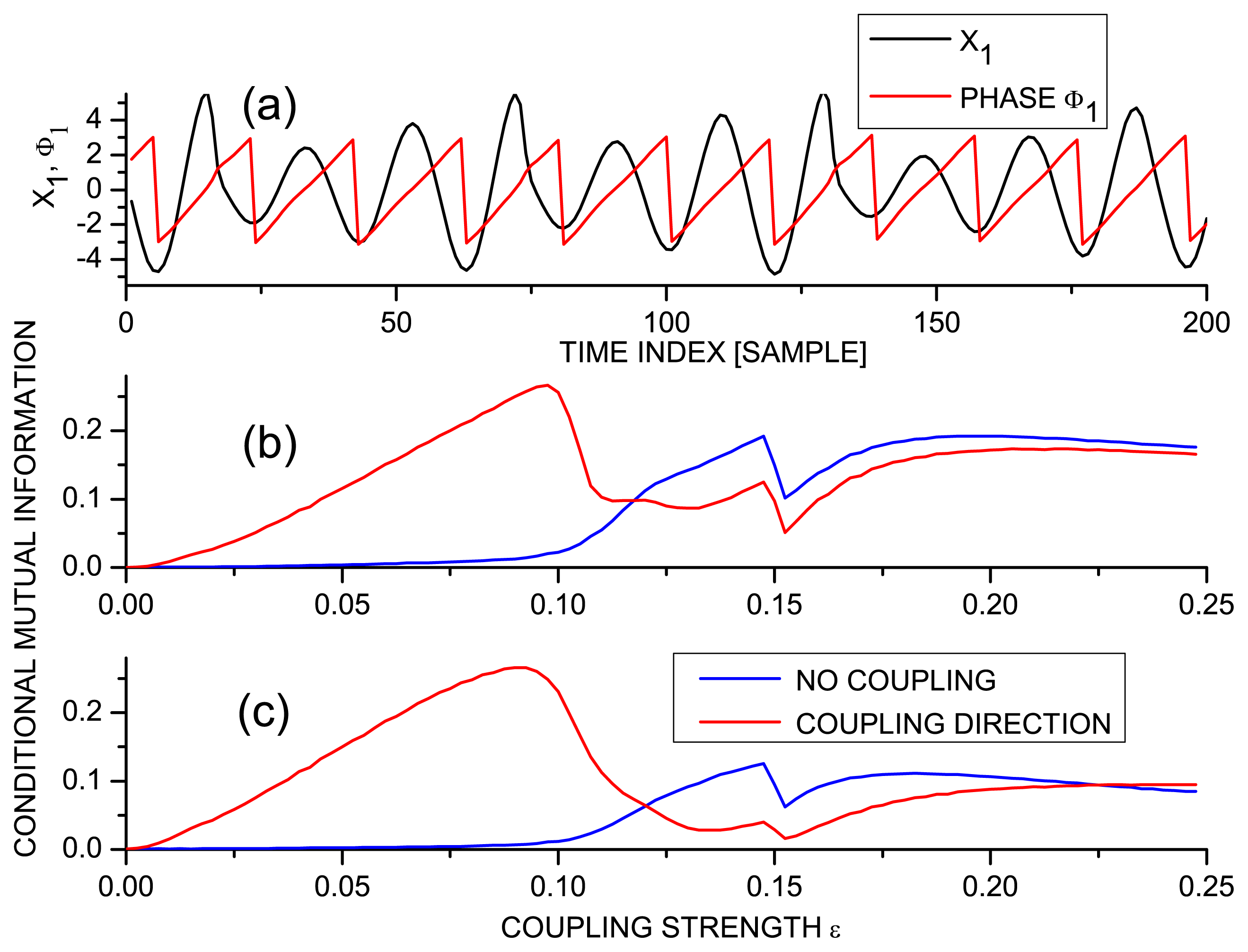
The chaotic solutions of the Rössler systems (13) and (14) oscillate in a relatively narrow frequency band (Figure 3a, black line), therefore it is possible to apply the Hilbert transform directly to the components x1 and y1 in order to obtain the instantaneous phases φ1 and φ2 of the driving system (13) and the driven system (14), respectively. Then the direction of coupling can be inferred using the conditional mutual information I(φ1(t); φ2(t + τ )|φ2(t)) and I(φ2(t); φ1(t + τ )|φ1(t)) already with the one-dimensional condition (Figure 3b) since the phase represents a simplified one-dimensional description of the Rössler system’s oscillations. Applying a higher-dimensional condition does not change the result (Figure 3c). Note that the one-dimensional condition is sufficient only for the “true” phase of self-sustained oscillators. A formally obtained phase φ(t) for a quasi-oscillatory component s(t) extracted from a multiscale system might require a condition of a higher dimensionality than one. Even in such a case, however, the conditioning dimension necessary for the phase φ(t) is typically lower than that required for the oscillatory component s(t).
2.5. Statistical Evaluation with Surrogate Data
Estimates of mutual information from finite number of samples are always nonzero. In the case of inferring directional coupling with the conditional mutual information (12), even with a sufficient dimension of the condition, the CMI estimates from finite number of samples are not only always nonzero but also always different in the two directions between the studied two systems. Considering possibly different biases, the absolute values of CMI estimates are not informative, but it is necessary to relate the CMI values computed from studied data to ranges of CMI values obtained from uncoupled processes that share important properties of analyzed data. This is the base of the surrogate data testing procedure in which we manipulate the original data in a randomization procedure that preserves original frequency spectra or variance on all relevant time scales; and the autocorrelation function in the cases of the Fourier transform (FT) surrogate data [41], or both the autocorrelation function and auto-mutual information function in the case of the multifractal (MF) surrogate data [42]. The surrogate data with the same sample spectrum as the tested time series can be constructed using the fast Fourier transform (FFT). The FFT of the series is computed, the magnitudes of the (complex) Fourier coefficients are kept unchanged, but their phases are randomized. The surrogate series is then obtained by computing the inverse transform into the time domain. Different realizations of the process are obtained using different sets of the random Fourier phases [41]. The discrete wavelet transform [43] is used for the generation of the multifractal surrogate data. The inspiration for this randomization procedure is the construction of a multifractal process using the wavelet dyadic trees proposed by Benzi et al. [44] and Arneodo et al. [45]. In particular, 2n wavelet coefficients on the scale
![Entropy 16 05263f12]() /2 are obtained by multiplying n coefficients on the scale
/2 are obtained by multiplying n coefficients on the scale
![Entropy 16 05263f12]() by a set of multiplicators, randomly drawn from a given distribution. After the construction of such a dyadic tree (always two different random multipliers are chosen in order to obtain two wavelet coefficients on a shorter scale from one wavelet coefficient on the closest larger scale), the inverse discrete wavelet transform produces a realization of a multifractal process mimicking information transfer from larger to smaller scales observed in turbulence. For construction of the multifractal surrogate data, a time series is transformed into a set of discrete wavelet coefficients and multipliers are computed by dividing each pair of coefficients on the scale
by a set of multiplicators, randomly drawn from a given distribution. After the construction of such a dyadic tree (always two different random multipliers are chosen in order to obtain two wavelet coefficients on a shorter scale from one wavelet coefficient on the closest larger scale), the inverse discrete wavelet transform produces a realization of a multifractal process mimicking information transfer from larger to smaller scales observed in turbulence. For construction of the multifractal surrogate data, a time series is transformed into a set of discrete wavelet coefficients and multipliers are computed by dividing each pair of coefficients on the scale
![Entropy 16 05263f12]() /2 by the related coefficient on the scale
/2 by the related coefficient on the scale
![Entropy 16 05263f12]() . Then, fixing one or two largest scales, the surrogate wavelet coefficients are recursively computed from larger to smaller scales using randomly permutated original multipliers. See [42] for details.
. Then, fixing one or two largest scales, the surrogate wavelet coefficients are recursively computed from larger to smaller scales using randomly permutated original multipliers. See [42] for details.
 /2 are obtained by multiplying n coefficients on the scale
by a set of multiplicators, randomly drawn from a given distribution. After the construction of such a dyadic tree (always two different random multipliers are chosen in order to obtain two wavelet coefficients on a shorter scale from one wavelet coefficient on the closest larger scale), the inverse discrete wavelet transform produces a realization of a multifractal process mimicking information transfer from larger to smaller scales observed in turbulence. For construction of the multifractal surrogate data, a time series is transformed into a set of discrete wavelet coefficients and multipliers are computed by dividing each pair of coefficients on the scale
/2 by the related coefficient on the scale
. Then, fixing one or two largest scales, the surrogate wavelet coefficients are recursively computed from larger to smaller scales using randomly permutated original multipliers. See [42] for details.
/2 are obtained by multiplying n coefficients on the scale
by a set of multiplicators, randomly drawn from a given distribution. After the construction of such a dyadic tree (always two different random multipliers are chosen in order to obtain two wavelet coefficients on a shorter scale from one wavelet coefficient on the closest larger scale), the inverse discrete wavelet transform produces a realization of a multifractal process mimicking information transfer from larger to smaller scales observed in turbulence. For construction of the multifractal surrogate data, a time series is transformed into a set of discrete wavelet coefficients and multipliers are computed by dividing each pair of coefficients on the scale
/2 by the related coefficient on the scale
. Then, fixing one or two largest scales, the surrogate wavelet coefficients are recursively computed from larger to smaller scales using randomly permutated original multipliers. See [42] for details.By construction, in the surrogate data the interactions between different time scales do not exist (FT surrogates), or only those explained by random cascades on wavelet dyadic trees are allowed (MF surrogates).
A pair of descriptors (phase–phase, amplitude–amplitude, phase–amplitude) reflecting the dynamics on two different time scales is chosen and their interactions are assessed by using the mutual information (5); or the conditional mutual information (12) is used for assessing the presence of directional, causal cross-scale coupling. The value Id of MI or CMI from the studied data is compared with the range of values Isi obtained from a set of surrogate data realizations. Having computed the mean
of the surrogate values Isi and their variance
, we can define the z-score
which is a measure how much the MI/CMI from the analyzed data differs from the range of MI/CMI for the surrogate data. The z-score usually gives a stable estimate from several tens of realizations (30–60) and its value can be related to the statistical significance, provided the Isi values have a normal distribution. Unfortunately, the latter is not always the case. Therefore we prefer to compute Isi from a larger number of realizations (1000 in this study) and construct an empirical surrogate data distribution as a histogram of Isi values. Using the cumulative histogram we estimate percentiles of the surrogate distribution and in each particular test we record the largest percentile of Isi distribution that is exceeded by Id from the analyzed data. We call this percentile “a significance level” since it is directly related to the significance of the statistical test based on the used surrogate data, irrespective of the surrogate Isi value distribution. For instance, the significance level 0.95 means that the Id value is significantly different from zero with the statistical significance p < 0.05.
The specificity of coupling or causality inference methods can be secured by an appropriate choice of surrogate data that reproduce the bias of an MI/CMI estimator applied to the studied data. The sensitivity of the method can be guaranteed by a certain bound on the estimator variance [26]. Typically, a lower variance requires a larger amount of data or, more precisely, a time series representing a longer epoch of evolution of the studied process [26,46].
3. Results and Discussion
3.1. Coping with Method Errors
Before applying the introduced methods to experimental data, we apply them to artificially generated data representing our null hypotheses. We demonstrate the systematic errors that the used wavelet decomposition can introduce and the way how the surrogate data test copes with these systematic errors.
For the first experiment, 65,536 samples of Gaussian white noise (GWN) were generated. CCWT with the Morlet wavelet was used to decompose the time series into components related to time scales (in samples) from
to
. Cross-scale phase–phase interactions were assessed using the mutual information I(φ1; φ2) where the phases φ1 were taken for the larger scales from 2436 to 23170 and the phases φ2 for the smaller scales from 181 to 1722 samples. The realization of GWN does not support any cross-scale interaction. Even though we compute I(φ1; φ2) with φ1 and φ2 for disjunct ranges of scales, in Figure 4a we can see areas of elevated values of I(φ1; φ2) in the upper left corner of the plot where the large and small scales are the closest (e.g., 2436 and 1722 samples). Clearly, this is a “leakage” of the wavelet transform producing dependent oscillatory modes for relatively close scales. Since this is an artifact of the CCWT, it is present also in Is(φ1; φ2) from the FT surrogate data (Figure 4b), which prevents to recognize the elevated values of I(φ1; φ2) in Figure 4a as statistically significant. Both the z-score (Figure 4c) and the significance levels (Figure 4d) show no significantly nonzero I(φ1; φ2). However, we need to recognize the multiplicity of the statistical tests—in Figure 4d we code in color each significant level greater than 0.95. It means that we display each pair of scales for which I(φ1; φ2) is statistically significant with p < 0.05 in a single test. In a large number of tests (combination of scales) we can encounter up to 5% of false positive results, appearing as randomly located spots in the significance plots.
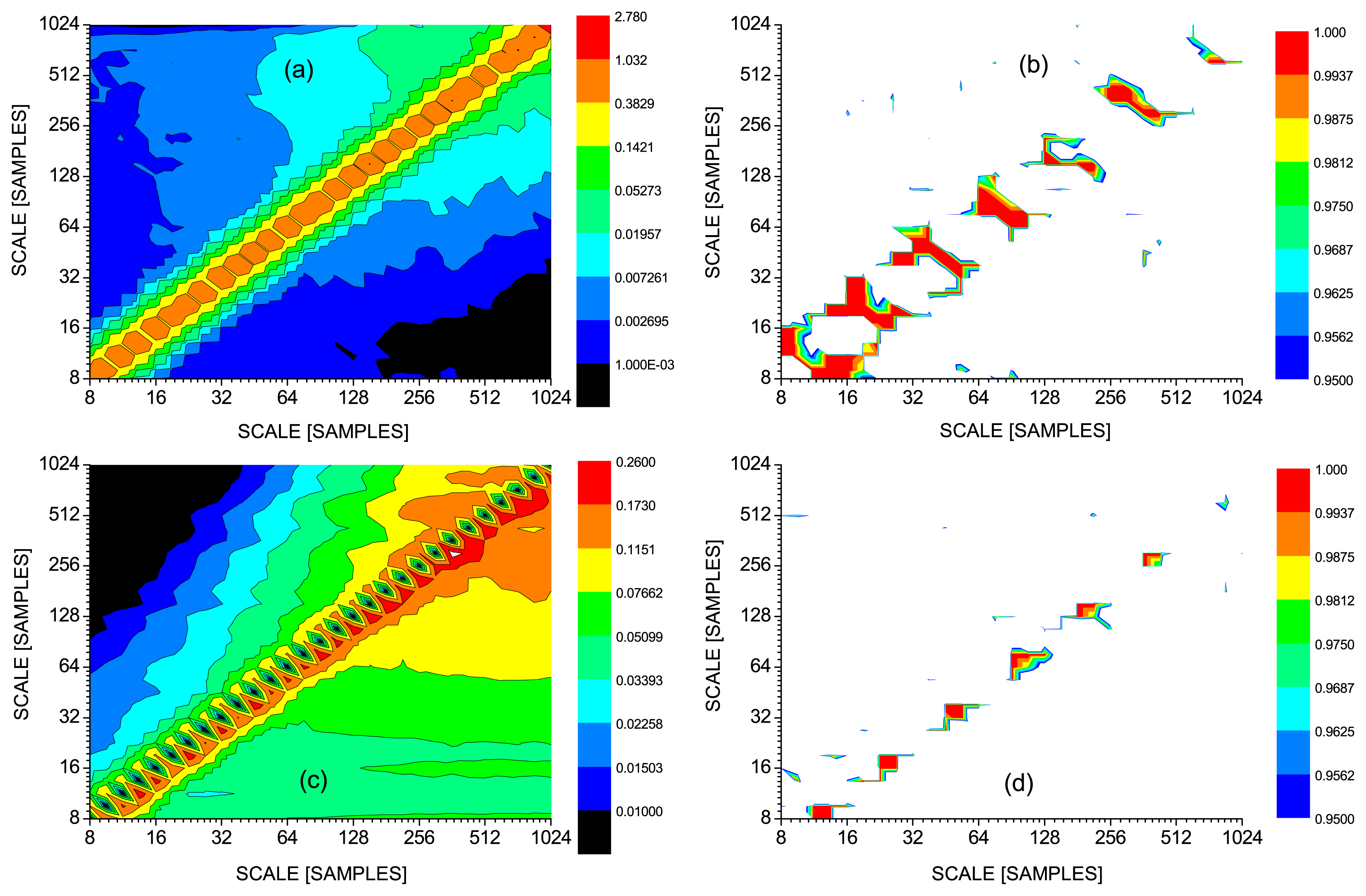
For the second experiment, a dyadic tree of wavelet coefficients is constructed using random multipliers with a log-normal distribution (see [42] for details). A 65,536-sample realization of a multifractal process is obtained by applying the inverse discrete wavelet transform. Then the generated multifractal time series is decomposed using the complex continuous wavelet transform. For the time scales from 8 to 1024 samples we will consider directly the wavelet components si(t) = Real{W(t, fi)} and again the phases φi(t), obtained according to Equation (16) with ŝi(t) = Im{W(t, fi)} as in the previous case. Figure 5a presents cross-scale interactions measured using the mutual information I(s1; s2). In this case we use the same range of scales (8–1024 samples) for both s1 and s2. Therefore the maximum I(s1; s2) is located in the diagonal where the two scales are identical. The MI I(s1; s2) decreases with increasing difference between the two scales; however, this decrease is slower for larger scales. From I(s1; s2) itself we cannot distinguish the cross-scale interactions in the multifractal data from the artifacts due to the CCWT. In order to detect cross-scale interactions in the studied multifractal process, we compare Id(s1; s2) from the multifractal data with its FT surrogate data. (Applying the MF surrogate data we would obtain similar patterns as in Figure 5a and no significant coupling as in Figure 4d.) The significance levels for Id(s1; s2) in Figure 5b show that the FT surrogates rule out the trivial dependence in the equal scales 8, 16, 32, ... samples, yet confirm the cross-scale interactions with the scale ratio 1:2 (i.e., the scales 8 and 16, or 16 and 32, etc., are coupled). In order to answer whether this coupling is symmetrical or directed, we study directed phase–phase interactions and apply the CMI I(φ1(t); φ2(t + τ )|φ2(t), φ2(t − η), φ2(t − 2η)) with the scale for φ1 on abscissa, and the scale for φ2 on ordinate. Again, the CMI itself (Figure 5c) shows an interesting pattern but it is not clear what are the true cross-scale interactions in the studied multifractal process. The true cross-scale interactions are uncovered by the significance levels for the CMI obtained using 1000 realizations of the FT surrogate data—in Figure 5d we can see that the scales close to 16 influence the scales close to 8 samples, and the scales close to 32 influence the scales close to 16 samples, etc. The CMI with the FT surrogate data confirmed the information transfer from a scale
![Entropy 16 05263f12]() to a scale
to a scale
![Entropy 16 05263f12]() /2, or from a time scale characterized by a frequency f to a time scale characterized by a frequency 2f. This information transfer does not reach over the closest smaller scale, i.e., it is restricted to the transfer of information from a certain scale to the next smaller scale approximately equal to one half of the preceding scale, exactly in the way how this realization of a multifractal process was constructed. This numerical construction based on the discrete wavelet transform (described above and in detail in [42]) uses scales given by the consecutive powers of two (2, 4, 8, 16, ... samples), while in the analysis we use the continuous (complex) wavelet transform that gives the possibility to study scales given by real numbers (limited by the available data). A closer look at Figure 5d reveals that there is no significant CMI at scales in the exact ratio 2:1. Apparently, the phases in the exact ratio 2:1 appear as phase-synchronized and the direction of coupling is not identifiable. However, there is always a range of close scales in which the significant CMI confirms the information transfer from scales close to
/2, or from a time scale characterized by a frequency f to a time scale characterized by a frequency 2f. This information transfer does not reach over the closest smaller scale, i.e., it is restricted to the transfer of information from a certain scale to the next smaller scale approximately equal to one half of the preceding scale, exactly in the way how this realization of a multifractal process was constructed. This numerical construction based on the discrete wavelet transform (described above and in detail in [42]) uses scales given by the consecutive powers of two (2, 4, 8, 16, ... samples), while in the analysis we use the continuous (complex) wavelet transform that gives the possibility to study scales given by real numbers (limited by the available data). A closer look at Figure 5d reveals that there is no significant CMI at scales in the exact ratio 2:1. Apparently, the phases in the exact ratio 2:1 appear as phase-synchronized and the direction of coupling is not identifiable. However, there is always a range of close scales in which the significant CMI confirms the information transfer from scales close to
![Entropy 16 05263f12]() to scales close to
to scales close to
![Entropy 16 05263f12]() /2, e.g., there is no significant CMI for the scales 16:8, but for the scales in ratios such as 15.488:8.712 the CMI is statistically significant (Figure 5d).
/2, e.g., there is no significant CMI for the scales 16:8, but for the scales in ratios such as 15.488:8.712 the CMI is statistically significant (Figure 5d).
to a scale
/2, or from a time scale characterized by a frequency f to a time scale characterized by a frequency 2f. This information transfer does not reach over the closest smaller scale, i.e., it is restricted to the transfer of information from a certain scale to the next smaller scale approximately equal to one half of the preceding scale, exactly in the way how this realization of a multifractal process was constructed. This numerical construction based on the discrete wavelet transform (described above and in detail in [42]) uses scales given by the consecutive powers of two (2, 4, 8, 16, ... samples), while in the analysis we use the continuous (complex) wavelet transform that gives the possibility to study scales given by real numbers (limited by the available data). A closer look at Figure 5d reveals that there is no significant CMI at scales in the exact ratio 2:1. Apparently, the phases in the exact ratio 2:1 appear as phase-synchronized and the direction of coupling is not identifiable. However, there is always a range of close scales in which the significant CMI confirms the information transfer from scales close to
to scales close to
/2, e.g., there is no significant CMI for the scales 16:8, but for the scales in ratios such as 15.488:8.712 the CMI is statistically significant (Figure 5d).We have estimated the CMI with increasing dimension of the condition from one (using I(φ1(t); φ2(t + τ )|φ2(t))) to three (using I(φ1(t); φ2(t + τ )|φ2(t), φ2(t − η), φ2(t − 2η)), with η equal to 1/4 of the scale of φ2). The CMI with the one- and two-dimensional condition brought a large rate of “false positives”, i.e., the cases of the significant CMI indicating the information transfer from smaller to larger scales. The conditioning dimension three appears as sufficient for the correct distinction of the direction of information transfer in the studied multifractal data.
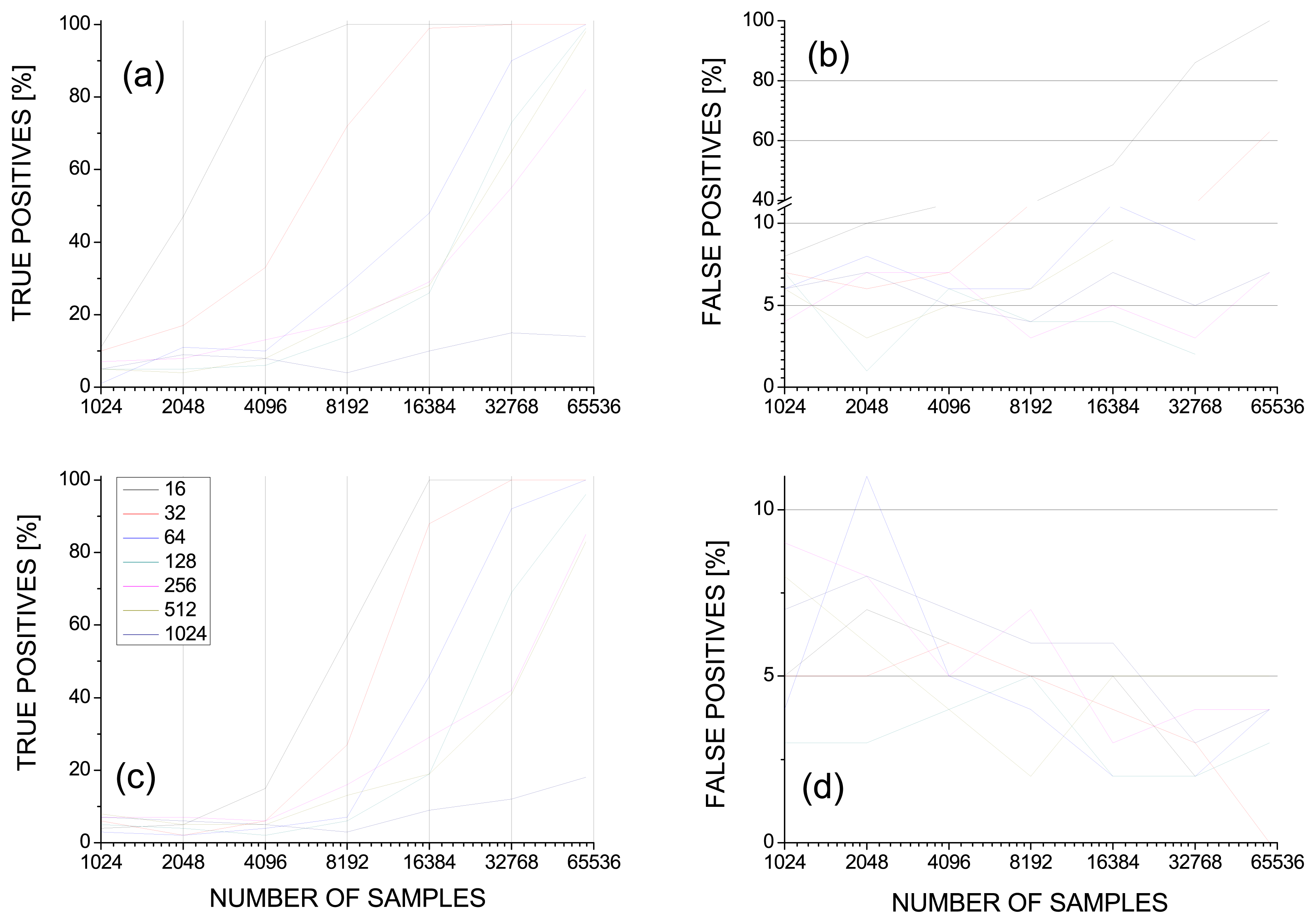
The CMI in this example was estimated using the equiquantal binning algorithm [14,26,46,47]. In order to assess the data requirements for a sensitive and specific inference of the information transfer, we have chosen 7 pairs of scales in the approximate ratio 2:1 and computed the CMI with different conditioning dimensions using different numbers of data samples (time series lengths) for 100 different realizations of the same multifractal process as that studied in Figure 5. The number of correctly detected information transfers from larger to smaller scales (“true positives”, i.e., the significant CMI in the direction of the existing information transfer from a larger to a smaller scale) gives the sensitivity of the test. The number of the significant CMI cases in the opposite direction (“false positives”, the significant CMI cases in the direction from smaller to larger scales) characterizes the specificity of the test. The results for I(φ1(t); φ2(t + τ )|φ2(t))with the one-dimensional condition (CMI-1D in the following) and I(φ1(t); φ2(t + τ )|φ2(t), φ2(t − η), φ2(t − 2η)) with the three-dimensional condition (CMI-3D) are presented in Figure 6. Considering the above observation that the information transfer direction cannot be inferred for the exact scale ratio 2:1, we have chosen the scale ratios 15.488:8.712; 31:17; 64:34; 124:68; 265:164; 432:296; 1039.64:534.64. Similar results, however, were obtained for a number of close scales representing the areas of the significant CMI in Figure 5d.
Figure 6 demonstrates that we need less data for the estimation of CMI-1D than for CMI-3D in order to obtain the 100% sensitivity in detecting the information transfer from larger to smaller scales in the studied multifractal process. Considering, e.g., the approximate scale ratio 16:8 (the black line in Figure 6), CMI-1D gives the 100% sensitivity using 8192 samples (or 90% sensitivity using 4096 samples). However, the rate of false positives is over 40%. In order to obtain the 100% sensitivity using the CMI-3D we need 16,384 samples, however, the rate of false positives is under 5%, which is the nominal significance level of the used test. The CMI-1D gives the test that is sensitive but not specific, since it suffers from a large rate of false positives. The results for CMI-2D are similar. Only CMI-3D provides the test that is specific and is sensitive enough using at least 16,384 samples for the scale ratio 16:8 (the black line), 32,768 samples for the scale ratio 32:16 (the red line in Figure 6), etc. Apparently, using the equiquantal binning estimator, the CMI-3D I(φ1(t); φ2(t + τ )|φ2(t), φ2(t − η), φ2(t − 2η)) gives a sensitive and specific indicator of the cross-scale information transfer if the analyzed time series contains, at least, approximately 1000 cycles of a slower oscillatory component. Unfortunately, such a requirement cannot be satisfied in many experimental studies and other approaches are necessary.
3.2. Cross-Scale Information Transfer in Atmospheric Dynamics
Uncovering interactions in the many scales of the dynamics of the Earth atmosphere and climate is one of the principal challenges of contemporary science with a potentially high impact for the society. In a search for a low-dimensional explanation of some scales of atmospheric dynamics, in the 1980s several researchers claimed detections of a weather or climate attractor of a low dimension [48–51]. Leading personalities of chaos theory, however, pointed to a limited reliability of chaos-identification algorithms and warned that the observed low-dimensional weather/climate attractors can be spurious [52,53]. Paluš & Novotná [54] even questioned the necessary condition for chaos—the presence of nonlinearity in the air temperature data when the dependence between a temperature time series {x(t)} and its lagged twin {x(t + τ )} was considered. Hlinka et al. [55] questioned nonlinearity in the dependence between the monthly time series of the gridded whole-Earth air temperature reanalysis data. It seems that linear correlation is a good descriptor for interactions in long-term air temperature recordings. Such data, however, reflect a very coarse view to a mixture of dynamics on many spatial and temporal scales. Considering specific spatial scales, a description of climate or weather variability using a low-dimensional nonlinear dynamical system can be plausible, as proposed by Tsonis and Elsner [56]. Recently, Tsonis [57] has uncovered that climate subsystems can act as pacemakers of decadal climate variability. The spatial scales for climate subsystems can be inferred from climate data using classical approaches of rotated principal component analysis combined with more recent surrogate data testing approach [58], or the very modern approach of complex networks [59]. Evolving climate networks can track important short-term climate influencing events such as El Niño episodes or large volcanic eruptions [60] and discern regional from global effects [61]. Besides considering specific spatial scales, a more detailed look on repetitive patterns on specific temporal scales in the air temperature and other meteorological data has led to an identification of oscillatory phenomena possibly possessing a nonlinear origin and exhibiting phase synchronization between oscillatory modes extracted either from different types of climate-related data or data recorded at different locations on the Earth [9–13,37]. Long-term air temperature recordings reflect complex atmospheric dynamics on multiple temporal scales. Oscillatory phenomena with the periods between 6 and 11 years, however, most frequently with the period around 7–8 years, have been observed in the air temperature and other meteorological data from European and Mediterranean areas by many authors (see [10,12] and references therein). Typically these oscillations are hidden in a red-noise background and their estimated amplitudes are small, therefore their relevance for the recent climate change has not been adequately assessed yet. We decided to study possible cross-scale interactions between oscillatory modes with periods between 6 and 12 years and variability with typical time scales from a few months to 4 years. The CCWT with the Morlet wavelet was used in order to obtain the instantaneous amplitudes and phases. We have not found any phase–phase interactions. Then we concentrated on the phase–amplitude coupling. In particular, we study a possible influence of the phase φ1 of slow oscillations on the amplitude A2 of higher-frequency variability, using the CMI functional
where τ is the forward time lag, η is the backward time lag in the m + 1-dimensional condition.
We use daily mean surface air temperature (SAT) time series recorded in various European locations. The data from Bamberg, Basel, De Bilt, Potsdam, Vienna and Zurich from the period 1901–1999 are a part of the data compiled for the European Climate Assessment [62]; the record from Prague-Klementinum is extended till 2008, and the SAT data from a number of German stations extended till 2011 are available due to the German Climate Data Center [63]. The inclusion criterion for this study is the availability of at least 90 years of uninterrupted daily mean SAT recording, since the computations of the CMI (21) have been performed using the time series length 32,768 daily samples. The relatively large amount of data was required in order to obtain reliable estimates and sensitive statistical tests, even though we used an estimator of the mutual information derived for Gaussian processes according to Equation (10). The functional (21) is evaluated and averaged for the forward lags τ from 1 to 750 days. (The CMI time-lag dependence is studied and discussed in the Supplemental Material of [64].) The backward lag η is set to 1/4 of the period of the slower oscillations characterized by the phase φ1, following the embedding construction recipe based on the first minimum of the mutual information [33].
The temporal evolution of the raw daily mean SAT data from mid-latitude locations is dominated by the annual cycle. In many climate-related studies deseasonalized SAT “anomalies” are used. In this study, however, we are interested in discovering interactions of all relevant temporal scales, therefore the raw SAT data are used for the computation of the CMI (21). The used surrogate data algorithms, however, might not accurately reproduce such a strong cyclic component. The latter is not consistent with the used multifractal model [42] and even the FT surrogate data procedure fails to reproduce a strong cyclicity and/or long coherence times [47]. Therefore, before the randomization, the seasonality in both mean and variance is removed from each SAT time series. This is done by computing the means and the variances for each calendar day. These seasonal means are subtracted from the raw SAT data of the corresponding days and the resultant SAT anomalies (SATA hereafter) are divided by the corresponding seasonal variances. Such deseasonalized data enter either the FT or MF randomization procedure. Then, the original seasonality in variance and mean is added back to each surrogate data realization. Each “seasonalized” surrogate realization undergoes the same processing procedure as the original SAT data—the CCWT is used to obtain the phase φ1 of slow oscillations and the amplitude A2 of higher-frequency variability, both used in the CMI (21) estimation. For each pair of the studied temporal scales, one thousand surrogate realizations are used for an empirical estimation of the percentiles of the CMI (21) surrogate distribution. As a result, we record the “significance level,” i.e., the highest percentile exceeded by the value of the CMI (21) computed from the original SAT data.
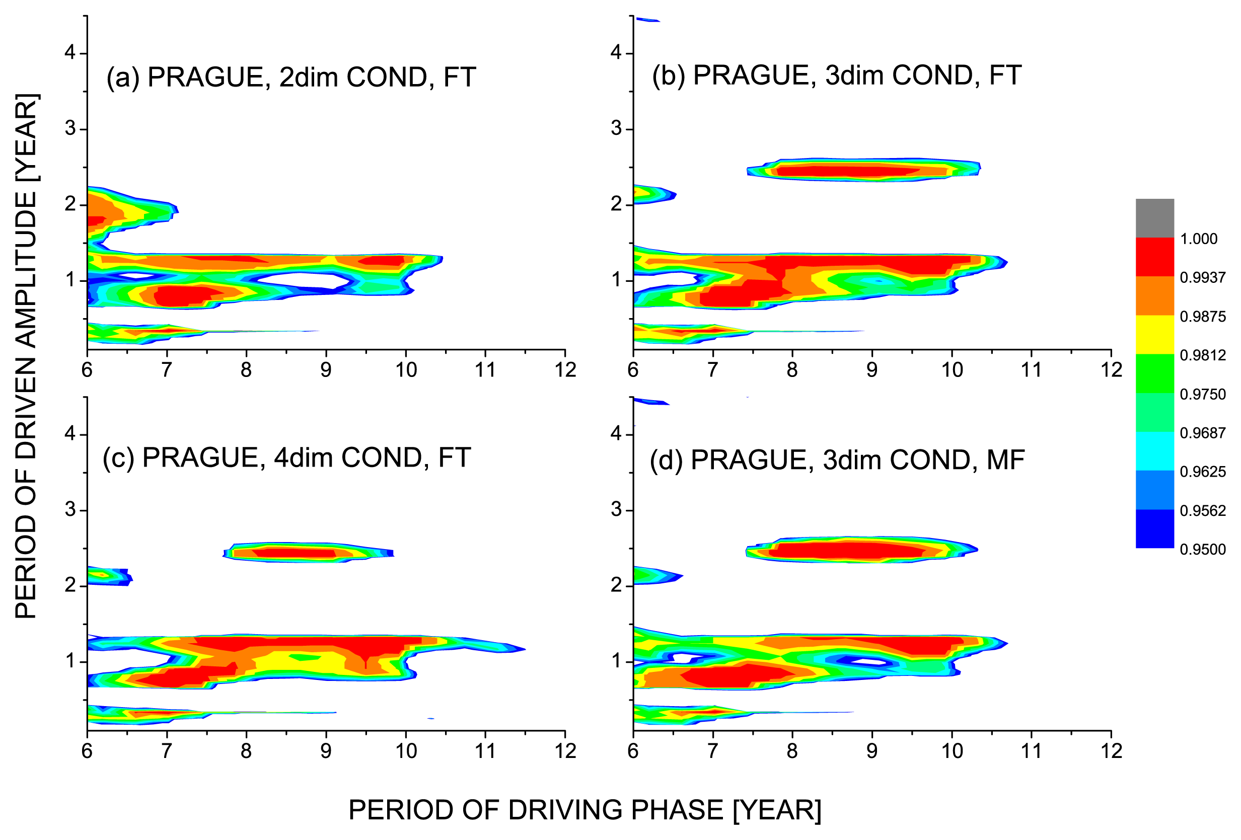
The significance levels for the CMI I(φ1(t);A2(t+τ )|A2(t), A2(t − η), . . ., A2(t − mη)) obtained from the Prague-Klementinum daily SAT data are presented in Figure 7. The results for the CMI with 2, 3 and 4 conditioning variables are depicted in Figure 7a–c, respectively. Since the increase of the conditioning dimension over three does not substantially change the patterns of φ1 → A2 interactions, the results for other European locations were obtained by evaluating I(φ1(t);A2(t + τ )|A2(t), A2(t − η), A2(t − 2η)) with the 3-dimensional condition. The tests with the two types of the surrogate data bring consistent results (cf. Figure 7b,d).
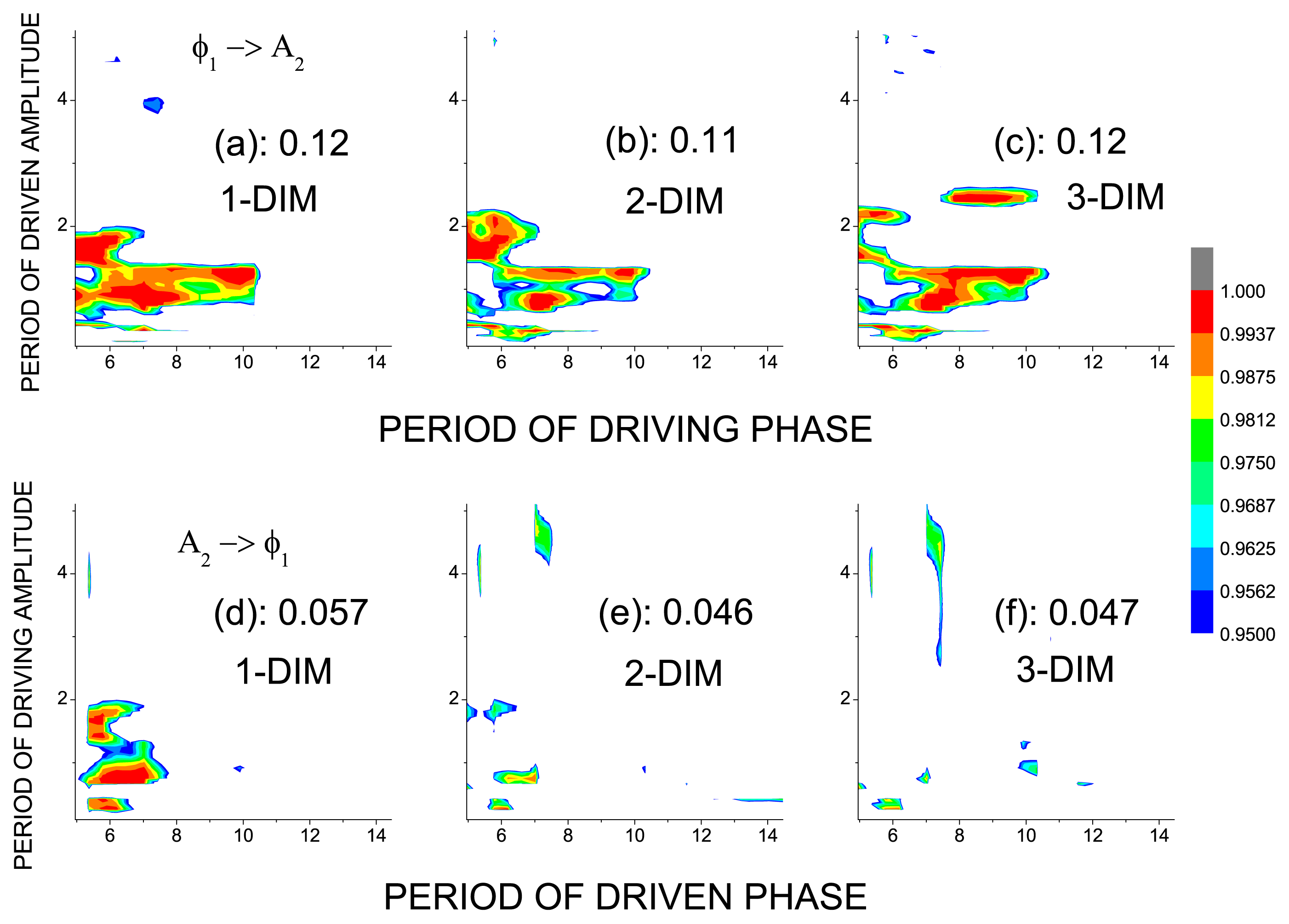
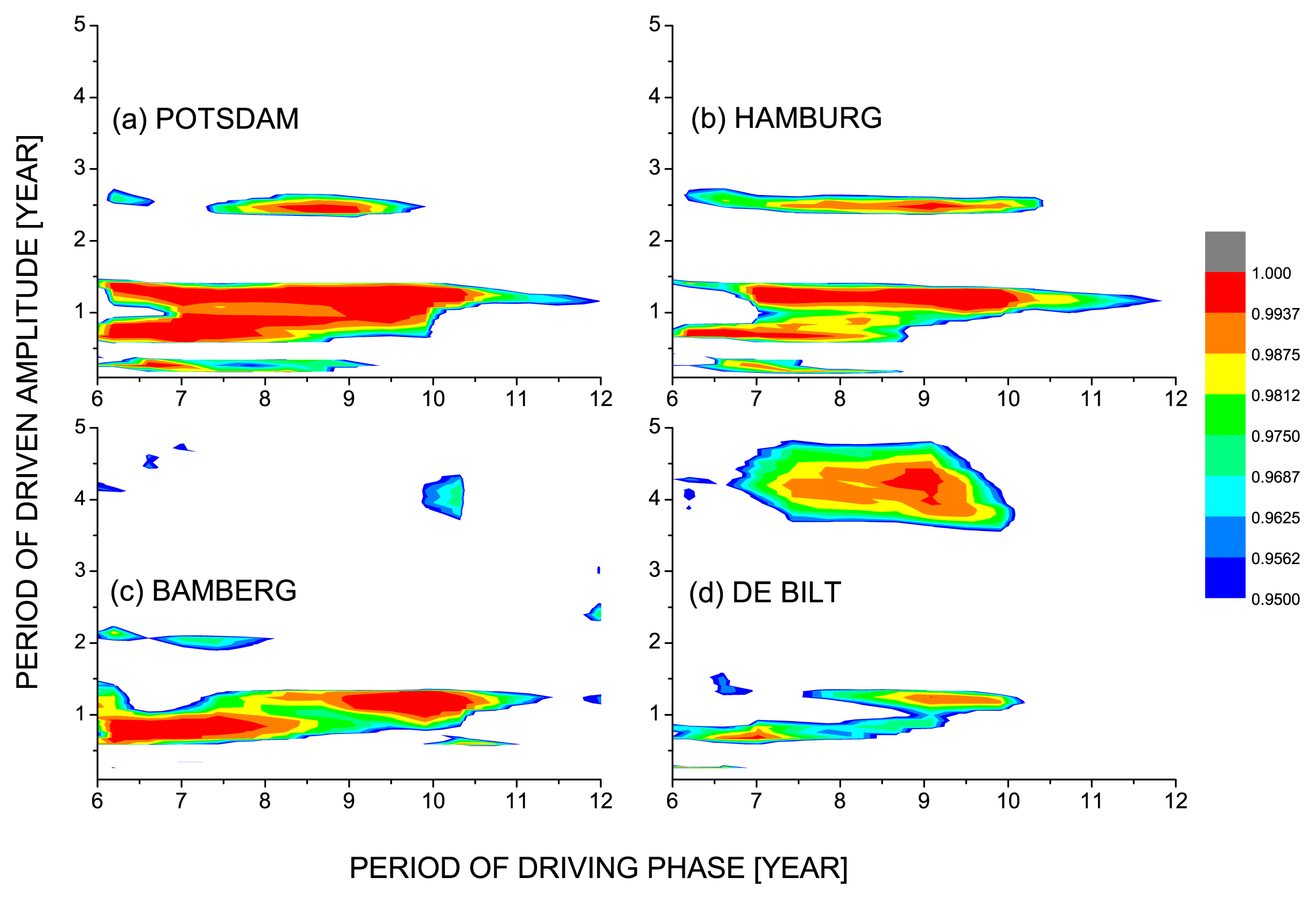
The choice of the three-dimensional condition does not mean that we consider the dimensionality of the amplitude dynamics equal to three, as in the case of the Rössler system, but that this dimension is sufficient for distinguishing a bidirectional from a unidirectional coupling in this case. Let us compare the results for I(φ1(t);A2(t + τ )|A2(t), A2(t − η), . . ., A2(t − mη)) measuring the directional coupling, or the information transfer in the direction φ1 → A2 with the CMI I(A2(t); φ1(t + τ )|φ1(t), φ1(t − η), . . . , φ1(t − mη)) in the opposite direction A2 → φ1 in Figure 8. Considering the significance level p < 0.05 for a single test, we obtain more than 10% of significant tests in the direction φ1 → A2 for all conditioning dimensions (Figure 8a–c), while in the direction A2 → φ1 there are more than 5% of significant results only in the case of the one-dimensional condition. From the conditioning dimension two, there is always less than 5% of significant results, which is the possible rate of false positives. Moreover, there is no consistent pattern of the (false) positives in the direction A2 → φ1 considering SAT data from different locations, while the pattern of the φ1 → A2 directional interactions is consistent in SAT recording from many locations in (mainly Central) Europe: The pattern of the φ1 → A2 directional interactions in SAT from Prague-Klementinum (longitude 14°25′E, latitude 50°05′N, Figure 7b) is almost the same as that from Potsdam (13°04′E, 52°23′N, Figure 9a) and very similar to the pattern from Hamburg (10°0′E, 53°33′N, Figure 9b).
Some changes can be seen in the pattern from Bamberg (10°53′E, 49°53′N, Figure 9c), while even more changes can be seen when approaching the Netherlands coast—De Bilt (05°11′E, 52°06′N, Figure 9d).
This observation supports the conclusion that in the dynamics (time evolution) of the air temperature there are unidirectional cross-scale interactions, or an information transfer from larger to smaller scales in the sense that the phase of slower oscillations causally influences the variability on shorter scales. These results provide a quantitative evidence for existence of previously unknown phenomenon in atmospheric physics. Understanding of its physical mechanisms is a challenge for further research.
The outputs of the statistical tests, however, are hard to understand in the sense of the effect of this phenomenon and its significance for weather and climate variability. We have already noted the existence of climate oscillations with the period around 7–8 years. References [10,12] give a brief review of observations of this cycle in instrumental as well as model meteorological data. Recently, the 7–8 years cycle has also been observed in soil and ground temperatures from a Prague area [65]. Figures 7 and 9 show that the phase of this cycle influences the air temperature variability in the scale between 2 and 3 years (quasicyclic variability also known as quasibiennial oscillations), at and around the annual cycle, and in short seasonal scales. The structure of the variability on these scales is an interesting topic for further research; here we will take a simplified look at the total temperature variability.
Let us consider the surface air temperature anomalies (SATA) from Prague-Klementinum and the instantaneous phase extracted from this SATA series using the CCWT with the central frequency giving the period 8 years. We can see a tendency of the temperature to have local maxima around the middle and minima near the beginning and the end of each 8-year cycle (Figure 10).
In order to assess a statistical association of the SATA variability and the 8-year cycle, we divide the phase in each 8-year cycle into 8 equidistant bins and compute the mean and variance of the SATA values for each of the eight bins. We obtain in this way the conditional SATA means and variances, conditioned by the phase of the 8-year cycle. If there is no statistical association between the SATA variability and the 8-year cycle, the conditional means and variances should be asymptotically the same. In the finite sample estimate, the conditional means and variances would fluctuate independently of the phase. However, this is not the case. In Figure 11 we can see that the years in the middle of the 8-year cycle are warmer and less variable, while the cycle edges are colder and the temperature is more variable. The MF surrogate data preserve the variance for particular scales, i.e., the presence of the cycle, but not the cross-scale interactions. From the surrogate results we can see that the cycle itself can explain the difference in yearly temperature means about 0.6 °C; however, in the data, the change of the mean temperature within the cycle reaches about 1.7 °C. In this way we can quantify the effect of the observed cross-scale interactions on the interannual temperature variability. This quantification, however, is not robust. It is nonstationary, changing in space and time, however, in the studied European locations, reaching values between 1 and 2 °C, which is a non-negligible variability.
4. Conclusions
Information theory provides useful tools for the detection of interactions in complex systems using experimental time series. A coupling (dependence) can be detected by using the mutual information (MI), while the conditional mutual information (CMI) can be used in the detection of directional coupling or causal interactions in the sense of Granger causality, generalized for nonlinear systems. CMI, also known as the transfer entropy, effectively measures a transfer of information from a system that influences the future of another system. Therefore the causal influence (in the Granger sense) is also interpreted as the information transfer. We have extended the methodology, originally developed to detect interactions and information transfer in the bivariate case of two systems, into the study of interactions between dynamical phenomena evolving on different time scales, however, forming together one complex, multiscale system. MI and CMI are applied to oscillatory components, extracted from a multiscale time series by using the complex continuous wavelet transform (CCWT). The oscillatory components are described using their instantaneous phases and amplitudes, so that various types of cross-scale interactions can be studied. Estimators of MI/CMI can be biased and CCWT can bring some systematic errors into the study of cross-scale interactions. Statistical testing based on surrogate data, however, can cope with these methodological errors. The specificity of surrogate data inference methods can be secured by an appropriate choice of surrogate data that reproduce the bias of a MI/CMI estimator applied to the studied data. The sensitivity of the method can be guaranteed by a certain bound on the estimator variance [26]. Typically, a lower variance requires a larger amount of data or, more precisely, a time series representing a longer epoch of evolution of the studied process [26,46]. The required time series length depends on the used MI/CMI estimator. A review of various estimators is given in [14], and the properties of several estimators in statistical tests are studied in [26,46].
The introduced method is demonstrated using simulated data. We identify cross-scale interactions in a model of a multifractal process that mimics information transfer from larger to smaller scales observed in turbulence. Then we apply the method to time series of long-term records of near-surface air temperature from a number of European locations. We report no cross-scale phase–phase interactions; however, we have reliably detected cross-scale phase–amplitude directed interactions. Here we need to make a remark about estimation algorithms and related data requirements for the sensitive tests for directed interactions. Considering cross-scale phase–phase interactions, we try to identify interactions of oscillations with different frequencies that are linearly independent. Therefore it is necessary to use a nonlinear MI/CMI estimator, which requires large amounts of data for multi-dimensional estimators used. Thus the phase–phase interactions in the studied atmospheric data either do not exist, or the available amount of data is not sufficient for a successful detection.
In the case of cross-scale phase–amplitude interactions, the situation is different. Even though the considered amplitude characterizes faster oscillations, the amplitude itself varies slowly, possibly within the same frequency range as the considered slow oscillations, characterized by the used phase. Therefore it is possible to use the MI/CMI estimator for Gaussian processes and to successfully detect, from the available data, the information transfer from larger to smaller time scales as the influence of the phase of slow oscillations on the amplitude of faster variability.
It is important that by increasing the conditioning dimension in the CMI we were able to prove the existence of an information transfer from larger to smaller scales but not vice versa. We have obtained quantitative support for the first condition of the Granger causality that the (phases of the) slow climate oscillations influence the future character of the fast temperature variability. We did not study, however, the second condition that the cause contains information about the effect that is unique, and is in no other variable. The mechanism of emergence of the 7–8 years oscillations in the air temperature dynamics in a large part of Europe is unknown yet and it is possible that its roots have a more global character. Then the observed directional coupling can be secondary, i.e., induced by another process. The answer to this question is a challenge for further research.
Acknowledgments
This study is supported by the Ministry of Education, Youth and Sports of the Czech Republic within the Program KONTAKT II, Project No. LH14001. Initial stages of this research were supported by the Czech Science Foundation, Project No. P103/11/J068.
Conflicts of Interest
The author declares no conflict of interest.
References
- Pikovsky, A.; Rosenblum, M.; Kurths, J. Synchronization. A Universal Concept in Nonlinear Sciences; Cambridge University Press: Cambridge, UK, 2001. [Google Scholar]
- Schäfer, C.; Rosenblum, M.G.; Kurths, J.; Abel, H.H. Heartbeat synchronized with ventilation. Nature 1998, 392, 239–240. [Google Scholar]
- Paluš, M.; Hoyer, D. Detecting nonlinearity and phase synchronization with surrogate data. IEEE Eng. Med. Biol. Mag 1998, 17, 40–45. [Google Scholar]
- Rodriguez, E.; George, N.; Lachaux, J.P.; Martinerie, J.; Renault, B.; Varela, F.J. Perception’s shadow: Long distance synchronization of human brain activity. Nature 1999, 397, 430–433. [Google Scholar]
- Paluš, M.; Komárek, V.; Hrnčíř, Z.; Štěrbová,, K. Synchronization as adjustment of information rates: Detection from bivariate time series. Phys. Rev. E 2001, 63, 046211. [Google Scholar]
- Paluš, M.; Komárek, V.; Procházka, T.; Hrnčíř, Z.; Štěrbová,, K. Synchronization and information flow in EEGs of epileptic patients. IEEE Eng. Med. Biol. Mag 2001, 20, 65–71. [Google Scholar]
- Lehnertz, K.; Bialonski, S.; Horstmann, M.T.; Krug, D.; Rothkegel, A.; Staniek, M.; Wagner, T. Synchronization phenomena in human epileptic brain networks. J. Neurosci. Methods 2009, 183, 42–48. [Google Scholar]
- Rybski, D.; Havlin, S.; Bunde, A. Phase synchronization in temperature and precipitation records. Phys. A 2003, 320, 601–610. [Google Scholar]
- Paluš, M.; Novotná, D. Quasi-biennial oscillations extracted from the monthly NAO index and temperature records are phase-synchronized. Nonlin. Processes Geophys 2006, 13, 287–296. [Google Scholar]
- Paluš, M.; Novotná, D. Phase-coherent oscillatory modes in solar and geomagnetic activity and climate variability. J. Atmos. Sol.-Terr. Phys 2009, 71, 923–930. [Google Scholar]
- Feliks, Y.; Ghil, M.; Robertson, A.W. Oscillatory climate modes in the Eastern Mediterranean and their synchronization with the North Atlantic Oscillation. J. Clim 2010, 23, 4060–4079. [Google Scholar]
- Paluš, M.; Novotná, D. Northern Hemisphere patterns of phase coherence between solar/geomagnetic activity and NCEP/NCAR and ERA40 near-surface air temperature in period 7–8 years oscillatory modes. Nonlin. Processes Geophys 2011, 18, 251–260. [Google Scholar]
- Feliks, Y.; Groth, A.; Robertson, A.W.; Ghil, M. Oscillatory climate modes in the Indian monsoon, North Atlantic, and Tropical Pacific. J. Clim 2013, 26, 9528–9544. [Google Scholar]
- Hlaváčková-Schindler, K.; Paluš, M.; Vejmelka, M.; Bhattacharya, J. Causality detection based on information-theoretic approaches in time series analysis. Phys. Rep 2007, 441, 1–46. [Google Scholar]
- Wiener, N. The theory of prediction. In Modern Mathematics for Engineers; Beckenbach, E., Ed.; McGraw-Hill: New York NY, USA, 1956. [Google Scholar]
- Granger, C.W.J. Time series analysis, cointegration, and applications. In Les Prix Nobel. The Nobel Prizes 2003; Frängsmyr, T., Ed.; Nobel Foundation: Stockholm, Sweden, 2004; pp. 360–366. [Google Scholar]
- Granger, C.W.J. Investigating causal relations by econometric models and cross spectral models. Econometrica 1969, 37, 424–438. [Google Scholar]
- Cover, T.; Thomas, J. Elements of Information Theory; J. Wiley: New York, NY, USA, 1991. [Google Scholar]
- Schreiber, T. Measuring information transfer. Phys. Rev. Lett 2000, 85, 461–464. [Google Scholar]
- Barnett, L.; Barrett, A.B.; Seth, A.K. Granger causality and transfer entropy are equivalent for Gaussian variables. Phys. Rev. Lett 2009, 103, 238701. [Google Scholar]
- Runge, J.; Heitzig, J.; Petoukhov, V.; Kurths, J. Escaping the curse of dimensionality in estimating multivariate transfer entropy. Phys. Rev. Lett 2012, 108, 258701. [Google Scholar]
- Kugiumtzis, D. Direct-coupling information measure from nonuniform embedding. Phys. Rev. E 2013, 87, 062918. [Google Scholar]
- Sun, J.; Bollt, E.M. Causation entropy identifies indirect influences, dominance of neighbors and anticipatory couplings. Phys. D 2014, 267, 49–57. [Google Scholar]
- Arnhold, J.; Grassberger, P.; Lehnertz, K.; Elger, C. A robust method for detecting interdependences: Application to intracranially recorded EEG. Phys. D 1999, 134, 419–430. [Google Scholar]
- Quiroga, R.Q.; Arnhold, J.; Grassberger, P. Learning driver-response relationships from synchronization patterns. Phys. Rev. E 2000, 61, 5142–5148. [Google Scholar]
- Paluš, M.; Vejmelka, M. Directionality of coupling from bivariate time series: How to avoid false causalities and missed connections. Phys. Rev. E 2007, 75, 056211. [Google Scholar]
- Chicharro, D.; Andrzejak, R.G. Reliable detection of directional couplings using rank statistics. Phys. Rev. E 2009, 80, 026217. [Google Scholar]
- Sugihara, G.; May, R.; Ye, H.; Hsieh, C.h.; Deyle, E.; Fogarty, M.; Munch,, S. Detecting Causality in Complex Ecosystems. Science 2012, 338, 496–500. [Google Scholar]
- Paluš, M. Detecting nonlinearity in multivariate time series. Phys. Lett. A 1996, 213, 138–147. [Google Scholar]
- Paluš, M.; Albrecht, V.; Dvořák, I. Information theoretic test for nonlinearity in time series. Phys. Lett. A 1993, 175, 203–209. [Google Scholar]
- Takens, F. Detecting strange attractors in turbulence. In Dynamical Systems and Turbulence, Warwick 1980; Rand, D.A., Young, L.S., Eds.; Lecture Notes in Mathematics; Springer: Berlin, Germany, 1981; Volume 898, pp. 366–381. [Google Scholar]
- Kocarev, L.; Parlitz, U. Generalized synchronization, predictability, and equivalence of unidirectionally coupled dynamical systems. Phys. Rev. Lett 1996, 76, 1816–1819. [Google Scholar]
- Fraser, A.M.; Swinney, H.L. Independent coordinates for strange attractors from mutual information. Phys. Rev. A 1986, 33, 1134–1140. [Google Scholar]
- Gans, F.; Schumann, A.Y.; Kantelhardt, J.W.; Penzel, T.; Fietze, I. Cross-modulated amplitudes and frequencies characterize interacting components in complex systems. Phys. Rev. Lett 2009, 102, 098701. [Google Scholar]
- Heil, C.; Walnut, D. Continuous and discrete wavelet transforms. SIAM Rev 1989, 31, 628–666. [Google Scholar]
- Huang, N.E.; Wu, Z. A review on Hilbert-Huang transform: Method and its applications to geophysical studies. Rev. Geophys 2008, 46. [Google Scholar] [CrossRef]
- Paluš, M.; Novotná, D. Enhanced Monte Carlo Singular System Analysis and detection of period 7.8 years oscillatory modes in the monthly NAO index and temperature records. Nonlin. Processes Geophys 2004, 11, 721–729. [Google Scholar]
- Paluš, M.; Novotná, D.; Tichavský, P. Shifts of seasons at the European mid-latitudes: Natural fluctuations correlated with the North Atlantic Oscillation. Geophys. Res. Lett 2005, 32, L12805. [Google Scholar]
- Torrence, C.; Compo, G.P. A practical guide to wavelet analysis. Bull. Am. Meteorol. Soc 1998, 79, 61–78. [Google Scholar]
- Jirsa, V.; Müller, V. Cross-frequency coupling in real and virtual brain networks. Front. Comput. Neurosci 2013, 7. [Google Scholar] [CrossRef]
- Theiler, J.; Eubank, S.; Longtin, A.; Galdrikian, B.; Farmer, J.D. Testing for nonlinearity in time series: the method of surrogate data. Phys. D 1992, 58, 77–94. [Google Scholar]
- Paluš, M. Bootstrapping multifractals: Surrogate data from random cascades on wavelet dyadic trees. Phys. Rev. Lett 2008, 101, 134101. [Google Scholar]
- Press, W.H.; Flannery, B.P.; Teukolsky, S.A.; Vetterling, W.T. Numerical Recipes: The Art of Scientific Computing; Cambridge University Press: Cambridge, UK, 1986. [Google Scholar]
- Benzi, R.; Biferale, L.; Crisanti, A.; Paladin, G.; Vergassola, M.; Vulpiani, A. A random process for the construction of multiaffine fields. Phys. D 1993, 65, 352–358. [Google Scholar]
- Arneodo, A.; Bacry, E.; Muzy, J.F. Random cascades on wavelet dyadic trees. J. Math. Phys 1998, 39. [Google Scholar] [CrossRef]
- Vejmelka, M.; Paluš, M. Inferring the directionality of coupling with conditional mutual information. Phys. Rev. E 2008, 77, 026214. [Google Scholar]
- Paluš, M. Testing for nonlinearity using redundancies—quantitative and qualitative aspects. Phys. D 1995, 80, 186–205. [Google Scholar]
- Nicolis, C.; Nicolis, G. Is there a climatic attractor? Nature 1984, 311, 529–532. [Google Scholar]
- Nicolis, C.; Nicolis, G. Evidence for climatic attractor. Nature 1987, 326, 529–532. [Google Scholar]
- Fraedrich, K. Estimating the dimensions of weather and climate attractors. J. Atmos. Sci 1986, 43, 419–432. [Google Scholar]
- Tsonis, A.A.; Elsner, J.B. The weather attractor over very short timescales. Nature 1988, 333, 545–547. [Google Scholar]
- Grassberger, P. Do climatic attractors exist? Nature 1986, 323, 609–612. [Google Scholar]
- Lorenz, E.N. Dimension of weather and climate attractors. Nature 1991, 353, 241–244. [Google Scholar]
- Paluš, M.; Novotná, D. Testing for nonlinearity in weather records. Phys. Lett. A 1994, 193, 67–74. [Google Scholar]
- Hlinka, J.; Hartman, D.; Vejmelka, M.; Novotná, D.; Paluš, M. Non-linear dependence and teleconnections in climate data: Sources, relevance, nonstationarity. Clim. Dyn 2014, 42, 1873–1886. [Google Scholar]
- Tsonis, A.A.; Elsner, J.B. Chaos, strange attractors, and weather. Bull. Am. Meteorol. Soc 1989, 70, 14–23. [Google Scholar]
- Tsonis, A.A. Climate Subsystems: Pacemakers of Decadal Climate Variability. In Extreme Events and Natural Hazards: The Complexity Perspective; Sharma, A.S., Bunde, A., Dimri, V.P., Baker, D.N., Eds.; American Geophysical Union: Washington D. C., USA, 2012; pp. 191–208. [Google Scholar]
- Vejmelka, M.; Pokorná, L.; Hlinka, J.; Hartman, D.; Jajcay, N.; Paluš, M. Non-random correlation structures and dimensionality reduction in multivariate climate data. Clim. Dyn 2014. [Google Scholar] [CrossRef]
- Tsonis, A.; Wang, G.; Swanson, K.; Rodrigues, F.; Costa, L. Community structure and dynamics in climate networks. Clim. Dyn 2011, 37, 933–940. [Google Scholar]
- Radebach, A.; Donner, R.V.; Runge, J.; Donges, J.F.; Kurths, J. Disentangling different types of El Niño episodes by evolving climate network analysis. Phys. Rev. E 2013, 88, 052807. [Google Scholar]
- Hlinka, J.; Hartman, D.; Jajcay, N.; Vejmelka, M.; Donner, R.; Marwan, N.; Kurths, J.; Paluš, M. Regional and inter-regional effects in evolving climate networks. Nonlin. Processes Geophys 2014, 21, 451–462. [Google Scholar]
- Klein Tank, A.M.G.; Wijngaard, J.B.; Können, G.P.; Böhm, R.; Demaree, G.; Gocheva, A.; Mileta, M.; Pashiardis, S.; Hejkrlik, L.; Kern-Hansen, C.; et al. Daily dataset of 20th-century surface air temperature and precipitation series for the European Climate Assessment. Int. J. Climatol 2002, 22, 1441–1453. [Google Scholar]
- Deutscher Wetterdienst of the German Federal Ministry of Transport, Building and Urban Development. Available online: http://www.dwd.de/ accessed on 21 September 2012.
- Paluš, M. Multiscale atmospheric dynamics: Cross-frequency phase-amplitude coupling in the air temperature. Phys. Rev. Lett 2014, 112, 078702. [Google Scholar]
- Čermák, V.; Bodri, L.; Šafanda, J.; Krešl, M.; Dědeček, P. Ground-air temperature tracking and multi-year cycles in the subsurface temperature time series at geothermal climate-change observatory. Stud. Geophys. Geod 2014, 58, 403–424. [Google Scholar]
Figure 1.
(a) Two largest Lyapunov exponents of the drive {X} (the constant lines) and the response {Y } (the decreasing curves); (b) the conditional mutual information I(x(t); y(t + τ )|y(t)) with the 1-dimensional condition, in the direction of coupling (full red line) and I(y(t); x(t + τ )|x(t)) in the direction without coupling (dashed blue line); (c) the conditional mutual information I(x(t); y(t + τ )|y(t), y(t − η), y(t − 2η)) with the 3-dimensional condition, in the direction of coupling (full red line) and I(y(t); x(t + τ )|x(t), x(t − η), x(t − 2η)) in the direction without coupling (dashed blue line); for the unidirectionally coupled Rössler systems (13) and (14), as functions of the coupling strength ε.

Figure 2.
An oscillatory mode with the central wavelet frequency giving the period of 8 years. Real (black) and imaginary (blue) components of the analytic signal, its instantaneous amplitude (envelope, red) and instantaneous phase (violet) are shown.
Figure 2.
An oscillatory mode with the central wavelet frequency giving the period of 8 years. Real (black) and imaginary (blue) components of the analytic signal, its instantaneous amplitude (envelope, red) and instantaneous phase (violet) are shown.

Figure 3.
(a) The component x1 (black line) of the Rössler system (13) and its instantaneous phase φ1 (red line). (b) The conditional mutual information I(φ1(t); φ2(t+τ)|φ2(t)) with the 1-dimensional condition, in the direction of coupling (red line) and I(φ2(t); φ1(t + τ )|φ1(t)) in the direction without coupling (blue line); (c) the conditional mutual information I(φ1(t); φ2(t + τ )|φ2(t), φ2(t − η), φ2(t − 2η)) with the 3-dimensional condition, in the direction of coupling (red line) and I(φ2(t); φ1(t + τ )|φ1(t), φ1(t − η), φ1(t − 2η)) in the direction without coupling (blue line); for the unidirectionally coupled Rössler systems (13) and (14), as functions of the coupling strength ε.

Figure 4.
(a) Cross-scale phase–phase interactions measured by I(φ1; φ2) for the Gaussian white noise (GWN) decomposed using the CCWT with the Morlet wavelet. (b) The mean Īs(φ1; φ2) for 1000 realizations of the FT surrogate data for the GWN data analyzed in (a). (c) z-score (color-coded for z > 2) and (d) significance levels (color-coded if they are greater than 0.95) for I(φ1; φ2) from (a) using 1000 realizations of the FT surrogate data.

Figure 5.
(a) Cross-scale interactions measured by I(s1; s2) for a multifractal process decomposed using the CCWT with the Morlet wavelet. (b) Significance levels (color-coded if they are greater than 0.95) for I(s1; s2) in (a) using 1000 realizations of the FT surrogate data. (c) Cross-scale phase–phase directed interactions—information transfer measured by I(φ1(t); φ2(t + τ )|φ2(t), φ2(t − η), φ2(t − 2η)) for a multifractal process. The scale for φ1 is on abscissa, the scale for φ2 is on ordinate. (d) Significance levels (color-coded if they are greater than 0.95) for I(φ1(t); φ2(t + τ )|φ2(t), φ2(t − η), φ2(t − 2η)) from (c) using 1000 realizations of the FT surrogate data.

Figure 6.
Sensitivity given by the “true positives” (a,c) and specificity given by the “false positives” (b,d) of the test for detecting the cross-scale phase–phase directed interactions—information transfer measured by CMI I(φ1(t); φ2(t + τ )|φ2(t))with the 1-dimensional condition (a,b) and CMI I(φ1(t); φ2(t + τ )|φ2(t), φ2(t − η), φ2(t − 2η)) with the 3-dimensional condition (c,d) for different scales in the approximate ratio 2:1, for the studied multifractal process. The legend assigns an approximate value of the larger scale to each line color used. The exact scales used are listed in the text. Note the different ordinate scales in (b,d).

Figure 7.
Causal influence of the phase of slower oscillations on the amplitude of faster fluctuations in the daily surface air temperature from Prague-Klementinum. The significance levels (color-coded if they are greater than 0.95) for the conditional mutual information I(φ1(t); A2(t + τ )|A2(t), A2(t − η), . . ., A2(t − mη)) with (a) 2-dimensional, (b,d) 3-dimensional, and (c) 4-dimensional condition, obtained using the (a–c) Fourier-transform, and (d) multifractal surrogate data.

Figure 8.
The significance levels (color-coded if they are greater than 0.95) for the conditional mutual information I(φ1(t);A2(t + τ )|A2(t), A2(t − η), . . ., A2(t − mη)) for the information transfer φ1 → A2 (a–c); and for CMI I(A2(t); φ1(t + τ )|φ1(t), φ1(t − η), . . . , φ1(t − mη)) in the opposite direction A2 → φ1 (d–f) with (a,d) 1-dimensional, (b,e) 2-dimensional, and (c,f) 3-dimensional condition for the daily surface air temperature from Prague-Klementinum. The numbers following the labels (a), (b), ..., are the ratios of numbers of statistically significant results to the total number of statistical tests in a figure.

Figure 9.
Causal influence of the phase of slower oscillations on the amplitude of faster fluctuations in the daily surface air temperature from (a) Potsdam, (b) Hamburg, (c) Bamberg, and (d) De Bilt. The significance levels for the conditional mutual information (21) with the 3-dimensional condition, obtained using the Fourier transform surrogate data, are color-coded if they are greater than 0.95.

Figure 10.
Smoothed (moving average with one-year moving window) daily SAT anomalies from Prague-Klementinum (red) and the instantaneous phase (blue) obtained from SATA series by using the CCWT with the central wavelet period 8 years.
Figure 10.
Smoothed (moving average with one-year moving window) daily SAT anomalies from Prague-Klementinum (red) and the instantaneous phase (blue) obtained from SATA series by using the CCWT with the central wavelet period 8 years.

Figure 11.
Conditional means (left panel, in °C) and conditional variances (right panel, in °C2) for the daily SAT anomalies from Prague-Klementinum (blue) and related MF surrogate data (red, with whiskers giving surrogate standard deviations) conditioned on the instantaneous phase obtained by using the CCWT with the central wavelet period 8 years, divided into eight equidistant bins.

© 2014 by the authors; licensee MDPI, Basel, Switzerland This article is an open access article distributed under the terms and conditions of the Creative Commons Attribution license (http://creativecommons.org/licenses/by/3.0/).
Share and Cite
MDPI and ACS Style
Paluš, M. Cross-Scale Interactions and Information Transfer. Entropy 2014, 16, 5263-5289. https://doi.org/10.3390/e16105263
AMA Style
Paluš M. Cross-Scale Interactions and Information Transfer. Entropy. 2014; 16(10):5263-5289. https://doi.org/10.3390/e16105263
Chicago/Turabian StylePaluš, Milan. 2014. "Cross-Scale Interactions and Information Transfer" Entropy 16, no. 10: 5263-5289. https://doi.org/10.3390/e16105263