Maximum Entropy Production vs. Kolmogorov-Sinai Entropy in a Constrained ASEP Model

Abstract
: The asymmetric simple exclusion process (ASEP) has become a paradigmatic toy-model of a non-equilibrium system, and much effort has been made in the past decades to compute exactly its statistics for given dynamical rules. Here, a different approach is developed; analogously to the equilibrium situation, we consider that the dynamical rules are not exactly known. Allowing for the transition rate to vary, we show that the dynamical rules that maximize the entropy production and those that maximise the rate of variation of the dynamical entropy, known as the Kolmogorov-Sinai entropy coincide with good accuracy. We study the dependence of this agreement on the size of the system and the couplings with the reservoirs, for the original ASEP and a variant with Langmuir kinetics.1. Introduction
The theory of dynamical systems at statistical equilibrium consists of well identified principles lying on firm mathematical foundations [1–3]. Although the representative point of the system in phase space (the microstate) can have a complicated dynamics, the statistics of any function on phase space (an observable) are well described, at least for large enough systems (in the thermodynamic limit) by simple invariant measures depending only on the invariants of the system, and not on the details of the dynamical equations. On the contrary, general theories describing the statistics of non-equilibrium systems are still in their infancy; although there have been attempts at formulating general principles governing non-equilibrium systems [4,5], they have not reached the level of mathematical rigor of their equilibrium counterpart, partly because there may not exist a universal way of being out-of-equilibrium, and remain valid essentially close to equilibrium.
Nevertheless, some progress have been achieved recently, in particular in the framework of “toy models”. Similarly to the Ising model which played a central role in the theory of critical phenomena, the so-called asymmetric simple exclusion process (ASEP) [6,7], which describes the transport of particles between two reservoirs, have become the dominant paradigm for non-equilibrium systems. Over the past few years, this system and others have benefited from the theory of large deviations, developed by Donsker and Varadhan [8–11]. This theory has introduced the large deviation function, which characterizes the statistics of the system in an asymptotic regime (large system, large time, low noise,...) and is a natural candidate for playing the out-of-equilibrium analogous role to the equilibrium free energy. In the long-time limit, the ASEP reaches a steady-state, and a macroscopic current is established between the two reservoirs. The average steady-state current, and the corresponding density profile, have been computed exactly [6,12,13], and more recently, the full large deviation function, which also describes the atypical fluctuations around these averages, has also been solved exactly [14], using a generalization of the matrix product ansatz.
Powerful as these techniques may be, they remain far from being applicable to more realistic systems. Indeed, if many systems in nature share some conceptual properties with the ASEP (establishment of a steady-state with fluctuations dominating the average behaviors and the resulting anomalous transport properties), not all of them are easily written as stochastic processes driven by a master equation. For instance, it has become clear over the years that deterministic systems with a very large number of degrees of freedom such as turbulent fluids, and in particular the atmosphere and the ocean of the Earth, should be thought of in terms of non-equilibrium statistical mechanics. However, up to now, attempts to apply such tools in the climate system have been restricted to phenomenological applications of the “Maximum Entropy Production” variational principle [15–17]. The success of these approaches points at a deeper connection with the general properties of non-equilibrium systems. A justification has been attempted [18], and dismissed [19,20], following the ideas of Jaynes that non-equilibrium systems should be characterized by a probability distribution on the trajectories in phase space, instead of just the points in phase space at equilibrium. In the context of Markov chains, this idea has proved to provide a natural generalization of equilibrium statistical mechanics [21], by considering the Kolmogorov-Sinai (KS) entropy. In this Letter, we establish a bridge between the phenomenological principle of maximum entropy production on the one hand, and the maximization of KS entropy on the other hand, in the context of the ASEP. We also consider a variant of the ASEP with Langmuir kinetics [22], which mimics the phenomenological climate model designed by Paltridge [15]. In both cases, rather than solving exactly the system for given dynamical rules, we show that the maxima location of the thermodynamic entropy production and the KS entropy as functions of the rate of transition coincide, and study the validity of this agreement when the system size and reservoir couplings vary.
2. Model Description
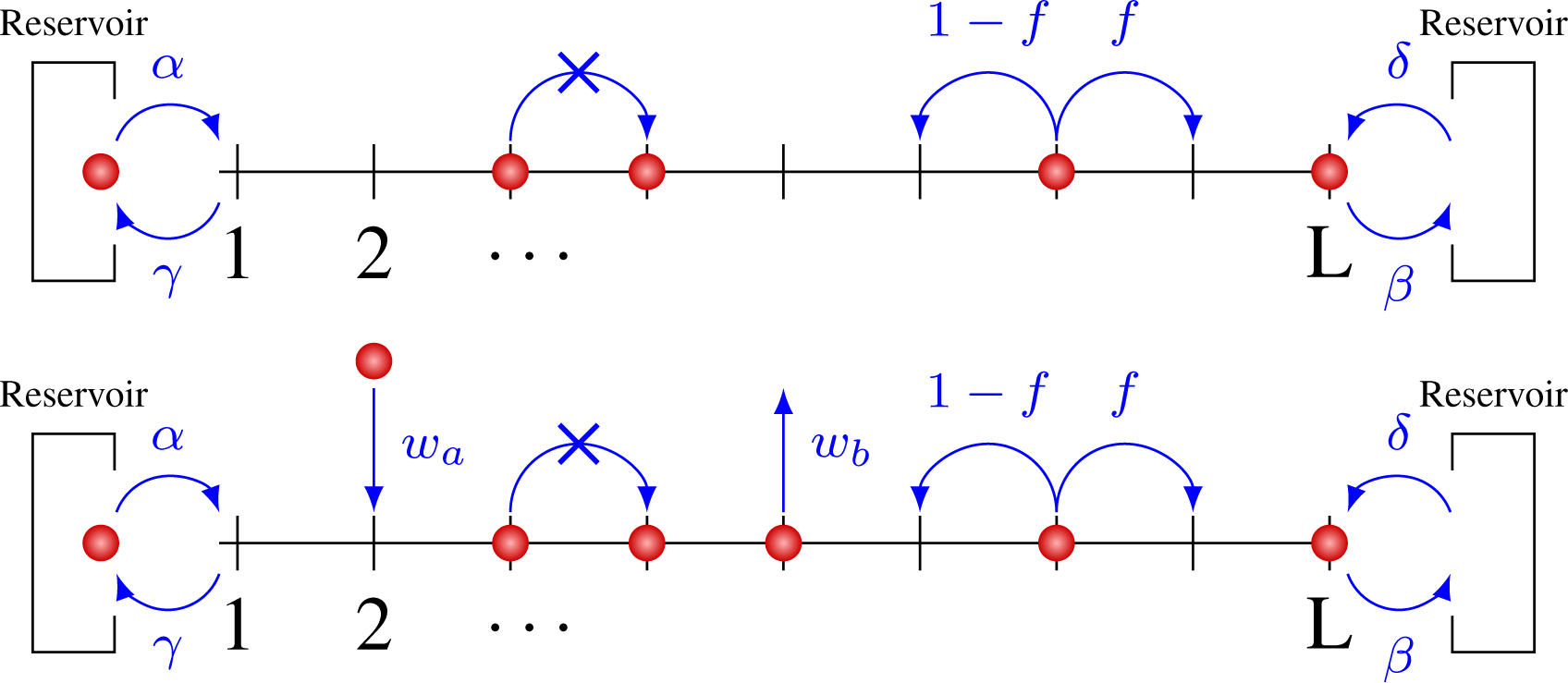
In this paper, we have considered a modified version to the ASEP model-hereafter named the CASEP model (for Changing ASEP model) or the LK-CASEP model when Langmuir dynamics is added-so as to be able to change the particle flux. A class of toy models for out-of-equilibrium systems consists of variants of the exclusion process (with open boundaries): let us consider a one dimensional lattice gas model composed of L sites between two reservoirs. Each site contains at most one particle. The particle undergoes a random walk on the lattice with the following rules: at each time step a site is chosen randomly. If this site belongs to the bulk and is occupied by a particle, the particle can jump right with a probability p and left with a probability q provided the neighboring sites are empty. At the boundaries, the system is coupled with the two reservoirs: at the left (resp. right) boundary, particles from the reservoir can enter the lattice with probability α and particles from the lattice can exit with probability γ (resp. δ and β). This coupling is equivalent to imposing the respective densities and . When ρa = ρb, the system reaches an equilibrium state, while it becomes increasingly out-of-equilibrium as the difference between ρa and ρb increases. The numerous variants of the exclusion process depend on choices of constraints on the hopping rates p and q: the symmetric simple exclusion process (SSEP) imposes p = q. Imposing a preferred direction for particle transport (e.g., p > q) yields the asymmetric simple exclusion model (ASEP). An extreme case is the totally asymmetric simple exclusion model (TASEP), for which q = 0. Here, we shall consider a particular class of ASEP, by imposing that the particle has to hop to a neighboring site—provided it is empty; it cannot remain in place unless both the neighboring sites are occupied (see Figure 1).
This amounts to setting p = f and q = 1 − f. We shall call this variant the Changing asymmetric simple exclusion process (CASEP).
The exclusion processes can be seen as microscopic models of transport. We are interested here in the connection with heat transport in turbulent flows at a macroscopic scale, like the atmosphere and the ocean. For such systems, phenomenological variational principles were suggested [15] to compute the energy transport associated with the establishment of a temperature gradient, outside of the diffusive regime. In the atmosphere, radiative exchanges on the vertical coexist with this meridional transport. To mimic this effect, we shall also consider a variant of the CASEP which includes Langmuir Kinetic dynamics (LK-CASEP) [22]: at each time step, particles can appear in an empty site with probability wa and disappear from an occupied site with probability wb.
The exclusion processes, and in particular the CASEP, are special cases of discrete Markov processes with 2L states. It is therefore difficult to study numerically this system for L larger than 10. These processes are characterized by their transition matrix P = (pij) which is irreducible. Thus, the probability measure on the states converges to the stationary probability measure μstat = ( , …, ) which satisfies:
Most of the studies of the ASEP model consider a fixed dynamics (given value for p and q) and try to solve exactly the resulting statistics for the steady-state current [14]. Here, we rather consider that the dynamics is not known exactly, and vary the parameter f in order to obtain different stationary states and calculate their entropy production σ function of f. Indeed, changing the parameter f is equivalent to change the flux of particles J. At fixed f, we can also use the dynamical properties of the CASEP model to compute the Kolmogorov-Sinai Entropy hKS as a function of f and compare it to σ(f).
In the case, the system reaches a steady state that is reminiscent of a “conductive state”, with a linear density behaviour over the lattice, going from on the left side to on the right side [6]. When , the system reaches another stationary state, ressembling a “convective state”, in which the density is mainly constant in the bulk, with steep transitions near the edges towards the left and the right side densities ρa and ρb.
3. Dynamical and Thermodynamical Entropy
We now define both the Macroscopic Entropy production and the Kolmogorov-Sinai Entropy for the CASEP model in order to compare them.
3.1. Komogorov-Sinai Entropy
There are many ways to estimate the Kolmogorov-Sinai entropy associated with a Markov chain [21,23]. Here we compute Kolmogorov-Sinai Entropy as the time derivative of the Jaynes Entropy. To characterize the dynamics of the system during the time interval [0, t], one considers the possible dynamical trajectories Γ[0,t] and the associated probabilities pΓ[0,t]. The dynamical trajectories entropy—the Jaynes entropy—reads:
3.2. Entropy Production
For a macroscopic system subject to thermodynamic forces Xi and fluxes Ji, the thermodynamics entropy production is given by [5,24]:
Thus, the entropy production reads:
4. Numerical Results
4.1. Comparison between KS Entropy and Macroscopic Entropy Production
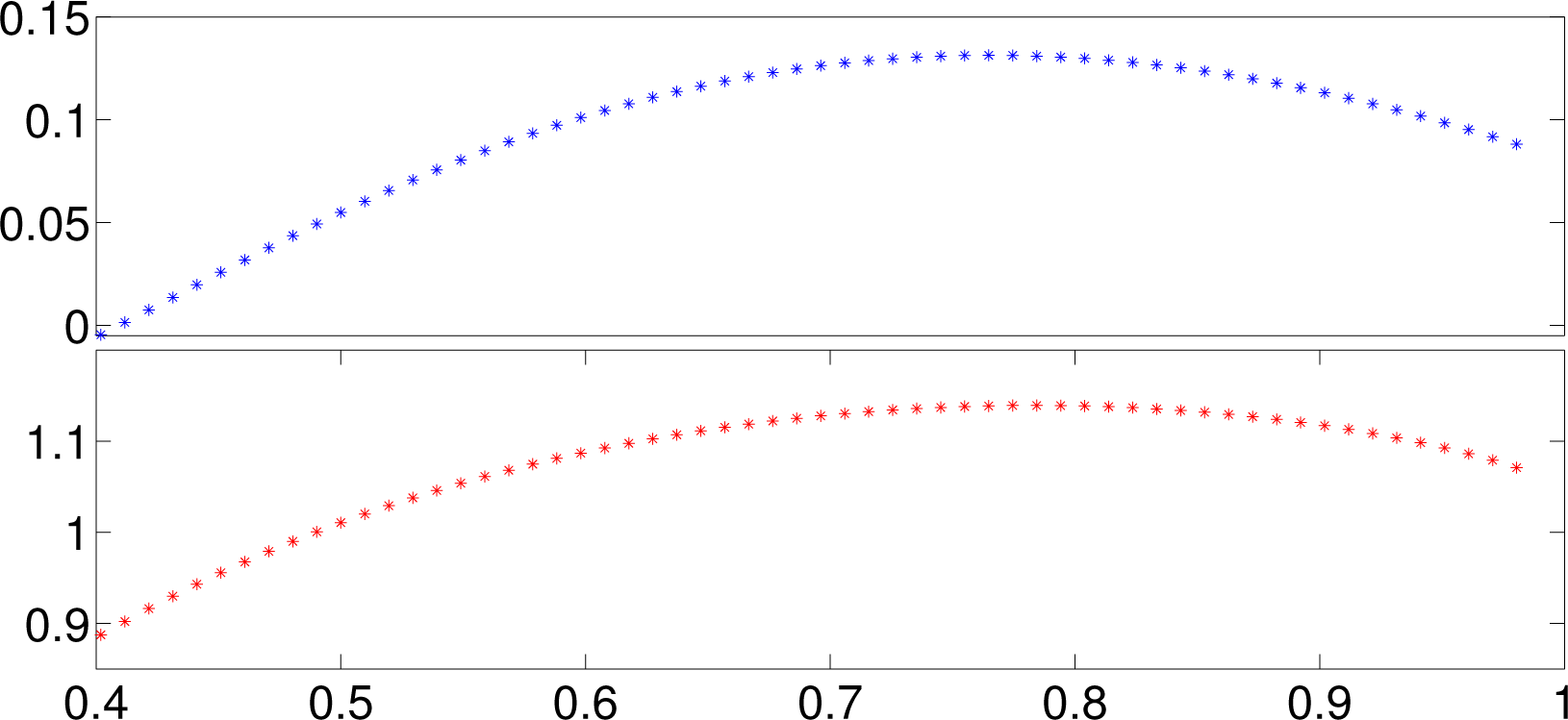
Given a value of L, ρa and ρb, we have computed the stationary states of the CASEP model as a function of f and used them to compute numerically the entropy production in Equation (6) and the Kolmogorov-Sinai Entropy in Equation (4). An example is provided in Figure 2 for ρa = 0.75, ρb = 0.1 and L = 10. We see that both function are of approximate parabolic shape, reaching a maximum for f ≥ 1/2. In the sequel, we note fmaxep (resp. fmaxks the value of f at which the maximum of the entropy production (resp. of the Kolmogorov-Sinai entropy) is reached. The existence of a maximum of entropy production can be simply understood by considering the case L = 2, i.e., a model with only two boxes, where we assume for simplicity that ρa > ρb. Noting ρ1 and ρ2 the density of the box number 1 and number 2 respectively, it is easy to see that for J = 0, σthermo = 0 whereas for J large enough ρ1 = ρ2 and σthermo = 0. Thus, in between these two values of J, σthermo has at least one maximum. We do not have such heuristic explanation for the existence of the maximum of the Kolmogorov-Sinai entropy. We note that although the entropy production and the Kolmogorov-Sinai entropy have similar parabolic shape, they do not coincide exactly: the entropy production and the Kolmogorov-Sinai entropy differ. For ρa = ρb (i.e., at equilibrium), their maxima take a common value fmaxep = fmaxks = 1/2, corresponding to the maximum of entropy: at equilibrium, all functionals are maximum for the same stationary state, corresponding to the “conductive state”. As the difference between ρa and ρb increases, the two maxima fmaxep and fmaxks deviates from the equilibrium value . This is the signature of a “convective dynamics”. We would like now to explore the behaviour of the two entropy around this conductive state, by studying the behaviour of the maxima difference, Δfmax=|fmaxep − fmaxks|.
4.2. Behaviour of the Maxima Difference
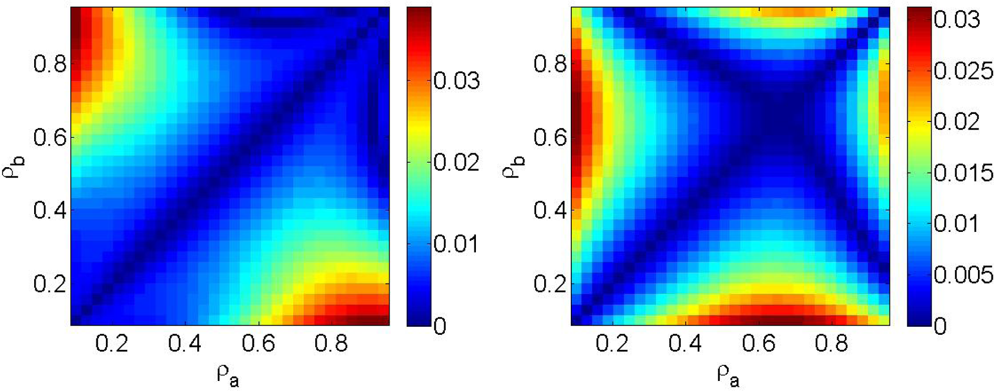
Let us first fix the size of the box, L, and study the variation of Δfmax=|fmaxep − fmaxks| as function of ρb and ρa. This is shown in Figure 3 (Left). It can be seen that Δfmax is zero for at perfect equilibrium, and remains small near equilibrium, for ρa ≈ ρb. The difference then increases as the system deviates from equilibrium, reaching a maximal value of about 4% at L = 10. These general features are conserved when including the Langmuir-Dynamics as can be seen in Figure 3 (Right): for L = 8 the difference between the maximum of entropy production and the maximum of the Kolmogorov-Sinai entropy also of the order of 4%. This is still valid varying wa and wb in [0, ]. These shows that the coincidence between the maxima of the KS entropy and the entropy production is robust and independent of inclusion of vertical fluxes.
4.3. Influence of Box Size
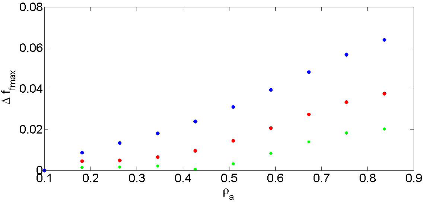
The previous results have been obtained for a number of boxes comparable with the number of boxes used in climate models. However, it is interesting to investigate possible finite size effects by varying L and observe the orresponding variations of Δfmax. Due to limited computational power, we were not able to simulate systems with L larger than L = 10. We could however decrease L and observe the result. This is done in Figure 4, where both fmaxep and fmaxks are plotted as a function of ρa and L for fixed ρb. One sees that for fixed ρa, the difference between the two values Δfmax decreases as L increases. So it is likely that for L → ∞, this quantity converges to 0 for any fixed ρa and ρb.
5. Discussion and Conclusions
In the present paper, we have built a bridge between stationary states that are maxima of Macroscopic Entropy production and maxima of Kolmogorov Sinai entropy, within a simple model of out-of-equilibrium physics. Both maxima coincide at equilibrium, and their difference increases with increasing out-of equilibrium. For fixed out-of-equilibrium conditions, however, the difference decreases with increasing system size. We may then postulate that for any fixed out-of-equilibrium conditions, both the Macroscopic Entropy production and the Kolmogorov Sinai entropy peak at the same stationary state, that thereby acquire a priviledged status. Whether such a stationary state is the natural one selected by the dynamics is actually an open question. Many studies point towards the relevence of the Kolmogorov Sinai entropy for out-of-equilibrium systems. For example, Latora and Baranger [25] established a link between the Kolmogorov-Sinai entropy, which is a microscopic quantity, with the derivative of the coarse grained entropy, which is a macroscopic quantity, in an out of equilibrium dynamical system. In the present paper, we have evidenced another connection between the Kolmogorov-Sinai entropy and a macroscopic quantity. This link, one hand, strengthens the hypothesis that Kolmogorov-Sinai entropy may play a key role in the study of out of equilibrium systems. On the other hand, its link with the Maximum Entropy Production may explain its rather successful role played in in many area of physics [26] such as solid physics [27], electromagnetism, quantum physics or climate science [15,17]. At present time, the connection has only been established for a 1D discrete special system. Generalizing our result to continuous ASEP model is straightforward, using the expression of the Kolmogorov-Sinai entropy found by [28]. However, it would be very interesting to generalize the link between maxima of Maximum Entropy Production and maxima of Kolmogorov-Sinai entropy to more complicated systems, such as chaotic dynamical systems, lattice Bolzmann or turbulent flows.
Acknowledgments
Martin Mihelich thanks IDEEX Paris-Saclay for financial support. We thank The National Center for Atmospheric Research which is sponsored by the National Science Foundation. The authors would like to thank the two anonymous reviewers whose comments help to clarify the manuscript.
Author Contributions
Each author contributed equally to this work.
Conflicts of Interest
The authors declare no conflicts of interest.
References
- Khinchin, A. The Mathematical Foundations of Statistical Mechanics; Dover Publications: New York, NY, USA, 1949. [Google Scholar]
- Ruelle, D. Statistical Mechanics: Rigorous Results; Benjamin: Amsterdam, The Netherlands, 1969. [Google Scholar]
- Ellis, R.S. Entropy, Large Deviations, and Statistical Mechanics; Springer: New York, NY, USA, 1985. [Google Scholar]
- Prigogine, I. Introduction to Thermodynamics of Irreversible Processes; Interscience: New York, NY, USA, 1967. [Google Scholar]
- De Groot, S.; Mazur, P. Non-Equilibrium Thermodynamics; Dover Publications: New York, NY, USA, 2011. [Google Scholar]
- Derrida, B. Non-equilibrium steady states: Fluctuations and large deviations of the density and of the current. J. Stat. Mech 2007. [Google Scholar] [CrossRef]
- Chou, T.; Mallick, K.; Zia, R.K.P. Non-equilibrium statistical mechanics: From a paradigmatic model to biological transport. Rep. Prog. Phys 2011, 74, 116601. [Google Scholar]
- Donsker, M.D.; Varadhan, S.R.S. Asymptotic evaluation of certain Markov process expectations for large time, I. Commun. Pure Appl. Math 1975, 28, 1–47. [Google Scholar]
- Donsker, M.D.; Varadhan, S.R.S. Asymptotic evaluation of certain Markov process expectations for large time, II. Commun. Pure Appl. Math 1975, 28, 279–301. [Google Scholar]
- Donsker, M.D.; Varadhan, S.R.S. Asymptotic evaluation of certain Markov process expectations for large time—III. Commun. Pure Appl. Math 1976, 29, 389–461. [Google Scholar]
- Donsker, M.D.; Varadhan, S.R.S. Asymptotic evaluation of certain Markov process expectations for large time. IV. Commun. Pure Appl. Math 1983, 36, 183–212. [Google Scholar]
- Schütz, G.M. Phase Transitions and Critical Phenomena; Domb, C., Lebowitz, J.L., Eds.; Academic: New York, NY, USA, 2001; Volume 19. [Google Scholar]
- Blythe, R.A.; Evans, M.R. Nonequilibrium steady sstates of matrix product form: A solver’s guide. J. Phys. A 2007, 40, 333–441. [Google Scholar]
- Gorissen, M.; Lazarescu, A.; Mallick, K.; Vanderzande, C. Exact current statistics of the asymmetric simple exclusion process with open boundaries. Phys. Rev. Lett 2012, 109, 170601. [Google Scholar]
- Paltridge, G.W. Global dynamics and climate—a system of minimum entropy exchange. Q. J. R. Meteorol. Soc 1975, 101, 475–484. [Google Scholar]
- Ozawa, H.; Ohmura, A.; Lorenz, R.; Pujol, T. The second law of thermodynamics and the global climate system: A review of the maximum entropy production principle. Rev. Geophys 2003, 41. [Google Scholar] [CrossRef]
- Herbert, C.; Paillard, D.; Kageyama, M.; Dubrulle, B. Present and Last Glacial Maximum climates as states of maximum entropy production. Q. J. R. Meteorol. Soc 2011, 137, 1059–1069. [Google Scholar]
- Dewar, R.C. Information theory explanation of the fluctuation theorem, maximum entropy production and self-organized criticality in non-equilibrium stationary states. J. Phys. A 2003, 36, 631–641. [Google Scholar]
- Grinstein, G.; Linsker, R. Comments on a derivation and application of the ‘maximum entropy production’ principle. J. Phys. A 2007, 40, 9717–9720. [Google Scholar]
- Bruers, S. A discussion on maximum entropy production and information theory. J. Phys. A 2007, 40, 7441–7450. [Google Scholar]
- Monthus, C. Non-equilibrium steady states: Maximization of the Shannon entropy associated with the distribution of dynamical trajectories in the presence of constraints. J. Stat. Mech 2011. [Google Scholar] [CrossRef]
- Parmeggiani, A.; Franosch, T.; Frey, E. Phase coexistence in driven one-dimensional transport. Phys. Rev. Lett 2003, 90, 086601. [Google Scholar]
- Billingsley, P. Ergodic Theory and Information; Wiley: Weinheim, Germany, 1965. [Google Scholar]
- Balian, R. Physique Statistique et Themodynamique Horséquilibre; (in French). Ecole Polytechnique: Palaiseau, France, 1992. [Google Scholar]
- Latora, V.; Baranger, M.; Rapisarda, A.; Tsallis, C. The rate of entropy increase at the edge of chaos. Phys. Lett. A 2000, 273, 97–103. [Google Scholar]
- Martyushev, L.M.; Seleznev, V.D. Maximum entropy production principle in physics, chemistry and biology. Phys. Rep 2006, 426, 1–45. [Google Scholar]
- Kirkaldy, J.S. Entropy criteria applied to pattern selection in systems with free boundaries. Metall. Mater. Trans. A 1985, 16, 1781–1797. [Google Scholar]
- Lecomte, V.; Appert-Rolland, C.; van Wijland, F. Thermodynamic formalism for systems with Markov dynamics. J. Stat. Phys 2007, 127, 51–106. [Google Scholar]


© 2014 by the authors; licensee MDPI, Basel, Switzerland This article is an open access article distributed under the terms and conditions of the Creative Commons Attribution license (http://creativecommons.org/licenses/by/3.0/).
Share and Cite
Mihelich, M.; Dubrulle, B.; Paillard, D.; Herbert, C. Maximum Entropy Production vs. Kolmogorov-Sinai Entropy in a Constrained ASEP Model. Entropy 2014, 16, 1037-1046. https://doi.org/10.3390/e16021037
Mihelich M, Dubrulle B, Paillard D, Herbert C. Maximum Entropy Production vs. Kolmogorov-Sinai Entropy in a Constrained ASEP Model. Entropy. 2014; 16(2):1037-1046. https://doi.org/10.3390/e16021037
Chicago/Turabian StyleMihelich, Martin, Bérengère Dubrulle, Didier Paillard, and Corentin Herbert. 2014. "Maximum Entropy Production vs. Kolmogorov-Sinai Entropy in a Constrained ASEP Model" Entropy 16, no. 2: 1037-1046. https://doi.org/10.3390/e16021037