The Application of Weighted Entropy Theory in Vulnerability Assessment and On-Line Reconfiguration Implementation of Microgrids

Abstract

With the consideration of randomness of distributed generations and loads, this paper has proposed a method for vulnerability assessment of microgrids based on complex network theory and entropy theory, which can explain the influence of the inherent structure characteristics and system internal energy distribution on the microgrid. The vulnerability assessment index is built, and the on-line reconfiguration model considering the vulnerability assessment of microgrid is also established. An improved cellular bat algorithm is tested on the CERTS system to implement the real time reconfiguration fast and accurately to provide the basis of theory and practice.

1. Introduction

Modern society has become more dependent on the secure distribution of electricity. The probability of incorrect operation may increase as a result of higher complexity when reinforcing the protection to guarantee dependability [1]. The vulnerability of the conventional power grid has been fully exposed by several outage accidents in recent years. Microgrids have been introduced as a promising solution due to their potential benefits to provide secure, stable and efficient environmentally friendly electricity, but vulnerability is an inherent property. The microgrid vulnerability is a measure of the weakness and the incidence of sections or lines with respect to cascading events. Analyzing and identifying the microgrid vulnerability on the basis of mathematical theory is the necessary precondition for monitoring and security control for future development.

The traditional procedure for static security assessment is concerned with the evaluation of a large number of contingency cases with a numerical algorithm. However, the vulnerability of microgrids varys randomly because of the dynamic operation of distributed generations, loads and power flow. Hence, finding an accurate vulnerability assessment method is very essential. In [2], the critical clearing time is defined as the vulnerability index to evaluate the power system based on EEAC method. Chen et al. [3] have presented the risk theory applied to the vulnerability assessment of power system based on probability theory. The power system was defined as a vulnerable system and a set of risk indices to assess the power system vulnerability and corresponding algorithm were built. In [4], Wang proposed the model of cascading failures as the foundation of vulnerability assessment and control. The fault chains are comparable from the aspects of vulnerability and cascading failures. The risk theory is introduced and the risk importance of fault chains. The risk importance of fault chains integrates the probabilities and consequences of occurrences of fault chains links, which are connected with many uncertain factors during the cascading outages. In [5] Li et al. have used the power flow entropy to assess the components vulnerability based on the principle of entropy and the distribution of power flow due to overload and removal of components. Sun [6] has suggested the recent blackouts throughout the world and the mechanism of cascading failures based on the summary of complex net work theory, including random network, small world network and scale free network.

A microgrid can operate in grid-connected or islanded mode. A successful transition between grid-connected and islanded modes and vice versa and a stable operation in both modes are very important for microgrid operation. MOLR is a type of dynamic control based on the instantaneous status in the microgrid including load shedding and adjusting, tie and sectionalizing switch changing, operation mode switching and other measures to redirect the power flow An implementation of MOLR is used to optimize the microgrid topology dynamically aiming at maximal stability, security and economic benefits.

In general, microgrid reconfiguration involves static reconfiguration and dynamic reconfiguration. The static reconfiguration is used to configure the power grid based on a fixed load value or the equivalent average load level, which usually focuses on an average load level and ignores overload and overvoltage during the operation moments. Mohd Zin et al. [7] have suggested a new heuristic method to optimize the network aiming at minimum branch currents of the system. A method for computing the sensitivities of the state variables with respect to switching operations for reconfiguration of radial networks has been presented in [8]. In [9], Rao et al. have proposed a novel method to solve the network reconfiguration problem in the presence of DG with an objective function of minimizing real power loss and improving voltage profile. A circular minimum-branch-current updating mechanism is proposed. Then, the best known configuration is obtained according to a circular neighbor-chain updating technique in [10]. However, dynamic reconfiguration optimizes the power grid according to the real time load state, which is suitable for microgrids due to its uniqueness discussed above. But now, most of the MOLR researches are suggested to divide the continuous period into several pieces of computation period, in which the average load value is used. The separated results are adopted for dynamic reconfiguration. Actually, the equivalent method belongs to static reconfiguration, called “Pseudo Dynamic Reconfiguration”. MOLR is proposed to provide the optimal configuration using real load forecasting based on the load status a moment before. Zhao et al. [11] have proposed a new reconfiguration algorithm based on dynamic particle swarm optimization. It adopts the voltage stability of the distribution system as the object function, and uses the improved particle swarm optimization algorithm which can trace dynamically the environment’s change to make the real time dynamically reconfiguration of distribution system. In [12], Wang et al. have used an interval algorithm for distribution network reconfiguration that aims at maximizing the confidence of energy loss reduction. Then it determines the optimal network structure in a day, which has the confidence measure of the maximal possibility evaluation of energy loss reduction. The algorithm can be utilized for the weekly network reconfiguration problem. In [13], the fault restoration optimization model of independent shipboard power system is proposed, and the Binary Particle Swarm Optimization (BPSO) is used for the optimization problem solution. In [9], a meta heuristic Harmony Search Algorithm (HSA) is used to simultaneously reconfigure. Liu et al. [14], have put forward a method of equivalent variable load on the entire time series, and then optimize it by static method. Besides, the algorithm is also one of the important parts of solving reconfiguration problems. Malekpour et al. [15] have used an adaptive particle swarm optimization (APSO) algorithm to obtain the optimal reconfiguration plan. Wu et al. [16] have proposed an enhanced integer coded particle swarm optimization (EICPSO) approach, to improve the search efficiency for feeder reconfiguration problems. Several other intelligent methodologies were presented in [17–21] for the feeder reconfiguration.

The reminder of this paper is organized as follows. Section 2 below provides the overviews on vulnerability assessment of microgrid. Section 3 describes the mathematical formulation of MOLR problem. The introduction of improved cellular bat algorithm and its application in MOLR problem is explained in Section 4. Section 5 presents the test results and Section 6 outlines the conclusions.

2. Vulnerability Assessment of Microgrid

2.1. Structure Vulnerability Index

The principle of the network topology can be described as follows: nodes stand for generators, loads and substations, and edges stand for lines [22–24]. R_i is introduced to be the weighted factor. The shortest path is defined as the minimum sum path between a generator and a node, which can be expressed as:

$$\mathit{Min}\sum _{i\in L}{R}_i$$

(1)

where R_i is the resistance at line i, L is the path set between two nodes.

In addition, the betweenness of nodes and lines B_n,i, B_l,i can be presented as the minimum sum of the shortest path going through node i or line i. Betweenness is an important part of the global geometric volume which reflects the role and the influence of node or edge in the entire network [25]. Betweenness is the measure of importance of the sections and also is one of the significant indexes for network structure vulnerability assessment.

2.2. Operation Vulnerability Index

Entropy is the measurement of the degree of confusion of a system [26,27]. It has been widely used in cybernetics, probability theory, astrophysics, life sciences, etc. In information theory, entropy value reflects the degree of disorder of the information, and it can be used to measure the amount of useful information. The bigger the entropy value, the more disordered the system is. Therefore, the entropy of the information can be used to evaluate the orderly degree and effectiveness of the information for a system. As a balanced system, the microgrid operation can be defined as the entropy of internal energy distribution, which is given as follows [28]:

$$H=-\sum _{i=1}^N{\varepsilon }_i\hspace{0.17em}\text{ln}\hspace{0.17em}{\varepsilon }_i$$

(2)

$${\varepsilon }_i=\frac{E_i}{E}$$

(3)

where ε_i is the rate of energy power distribution of i th unit; H is the energy entropy; E_i is the energy power of i th unit; E is the total energy power; N is the number of units.

The vulnerability of a microgrid is described as the ability to maintain the stability of network structure when one element or some elements are out of operation. The microgrid entropy value shows the rule of energy average distribution. The disturbance impacts aggregate on some elements in the case of elements out of operation, which means unbalanced microgrid energy distribution. Additionally, the smaller the entropy value is, the microgrid becomes more vulnerable, and vice versa.

2.2.1. Nodes Vulnerability Assessment Index

A microgrid aims at providing diverse power quality for users. The bus voltage changes quickly once the system state changes or faults happen. Different kinds of bus have different power quality demand, especially the sensitive loads. For bus voltage, the i th nodes entropy vulnerability assessment index VI_l,i is:

$$V{I}_{1,i}=\frac{\Delta V_i}{H_1\left(i\right)}=\frac{\Delta V_{i,i}+\sum _{j=1,j\ne i}^{N_n}\Delta V_{j,i}}{H_1\left(i\right)}$$

(4)

$$\Delta V_{i,i}=\left|V_{i,i}\left(t\right)-V_{i,\mathit{ref}}\right|$$

(5)

where ΔV_i represents the total voltage deviation caused by bus i; ΔV_i,i is the self voltage deviation of bus i; ΔV_j,i is the voltage deviation of bus j caused by bus i; N_n is the number of buses; V_i,i (t) is the voltage of i th bus at time t; V_{i, ref}is the specified voltage magnitude at bus i; H₁ (i) is the entropy value of i th bus. ε_1,i is described as the ratio of i th node voltage deviation and total nodes voltage deviation caused by i th node, which is given below:

$${\varepsilon }_{1,i}=\frac{\Delta V_{i,i}}{\Delta V_i}$$

(6)

2.2.2. Line Vulnerability Assessment Index

The microgrid is designed based on the concept of the system energy demand. Line vulnerability assessment index VI_2,i is used to guarantee the energy transmission in case of line overload, power flow disturbance or fault [29]. However, the traditional line vulnerability assessment index only pays attention to active power without considering the reactive power. The line entropy vulnerability assessment index considering (cos δ_i)² and (sin δ_i)² as the weighted factors is given below:

$$V{I}_{2,i}=\frac{\Delta {\mathit{OL}}_i}{H_S\left(i\right)}={\left(\text{cos}\hspace{0.17em}{\delta }_i\right)}^2\frac{\Delta {\mathit{OL}}_{pi}}{H_P\left(i\right)}+{\left(\text{sin}\hspace{0.17em}{\delta }_i\right)}^2\frac{\Delta {\mathit{OL}}_{qi}}{H_Q\left(i\right)}=\frac{{\left(\text{cos}\hspace{0.17em}{\delta }_i\right)}^2\frac{P_i}{P_{i,\mathit{cap}}}+\sum _{j=1,\hspace{0.17em}\hspace{0.17em}j\ne i}^{N_l}{\left(\text{cos}\hspace{0.17em}{\delta }_j\right)}^2\frac{P_{j,i}}{P_{j,\mathit{cap}}}}{H_p\left(i\right)}+\frac{{\left(\text{sin}\hspace{0.17em}{\delta }_i\right)}^2\frac{Q_i}{Q_{i,\mathit{cap}}}+\sum _{j=1,\hspace{0.17em}\hspace{0.17em}j\ne i}^{N_l}{\left(\text{sin}\hspace{0.17em}{\delta }_j\right)}^2\frac{Q_{j,i}}{Q_{j,\mathit{cap}}}}{H_Q\left(i\right)}$$

(7)

$${\delta }_i=\text{arctan}\left(\frac{X_i}{R_i}\right)$$

(8)

where, ΔOL_i represents the complex power overload rate of i th line; δ_i is the impedance angle of line i; H _S (i) is the entropy value of i th line; N_l is the number of lines; X_i is the reactance of line i; R_i is the resistance of line i; ΔOL_pi, ΔOL_qi are the active and reactive power overload rate of i th line, respectively; H _P (i), H _Q (i) are the active and reactive power entropy of line i, respectively; P_j,i, Q_j,i are the active and reactive power of j th line; N_l is the number of lines; P_i,cap, Q_i,cap represent the active and reactive power capacity of line i; P_i, Q_i, are the active and reactive power of i th line; In equation (7), the variation of active and reactive power can be represented as the sum of the self overload rate of line i$\frac{P_i}{P_{i,\text{cap}}},\frac{Q_i}{Q_{i,\text{cap}}}\hspace{0.17em}$ and the overload rate of other lines caused by line i, $\sum _{j=1,j\ne i}^{N_1}\frac{P_{j,i}}{P_{j,\text{cap}}},\hspace{0.17em}\sum _{j=1,j\ne i}^{N_1}\frac{Q_{j,i}}{Q_{j,\text{cap}}}$, respectively

In addition, ε_2,i is described as the ratio of i th line power deviation and total power deviation caused by i th line, which is given below:

$${\varepsilon }_{2,pi}=\frac{\Delta P_i}{\Delta P},{\varepsilon }_{2,qi}=\frac{\Delta Q_i}{\Delta Q}$$

(9)

where, ε_{2, pi}, ε_{2, qi} the active energy power and reactive energy power of i th line, respectively; ΔP_i, ΔQ_i, are the active and reactive power change of line i, respectively; ΔP, ΔQ are the Total active and reactive power change, respectively.

2.3. System Vulnerability Assessment Index of Microgrid

The betweenness value can stand for the importance of the nodes or lines. Moreover, the bigger the ΔV_i is, the higher the aggregative degree of disturbance is, the smaller entropy value H ₁ (i) is, and the bigger the vulnerability index is. Finally, define the whole vulnerability value of a microgrid as the sum of weighted VI_1,i with VI_2,i. The B_i is considered as a weighted factor. The total vulnerability value ISV of the microgrid can be expressed below:

$$\mathit{ISV}={\omega }_1\sum _{i=1}^{N_n}{B}_{n,i}{\mathit{VI}}_{1,i}+{\omega }_2\sum _{i=1}^{N_l}{B}_{l,i}{\mathit{VI}}_{2,i}={\omega }_1\sum _{I=1}^{N_N}{B}_{ni}\frac{\Delta V_i+\sum _{j=1,j\ne i}^{N_n}\Delta V_j}{H_1\left(i\right)}+{\omega }_2\sum _{k=1}^{N_t}{B}_{l,k}[\frac{{\left(\text{cos}\hspace{0.17em}{\delta }_i\right)}^2\frac{P_i}{P_{i,\mathit{cap}}}+\sum _{j=1,\hspace{0.17em}\hspace{0.17em}j\ne i}^{N_l}{\left(\text{cos}\hspace{0.17em}{\delta }_j\right)}^2\frac{P_{j,i}}{P_{j,\mathit{cap}}}}{H_{\tilde{P}}\left(i\right)}+\frac{{\left(\text{sin}\hspace{0.17em}{\delta }_i\right)}^2\frac{Q_i}{Q_{\mathit{cap}}}+\sum _{j=1,\hspace{0.17em}\hspace{0.17em}j\ne i}^{N_l}{\left(\text{sin}\hspace{0.17em}{\delta }_j\right)}^2\frac{Q_{j,i}}{Q_{j,\mathit{cap}}}}{H_{\tilde{Q}}\left(i\right)}]$$

(10)

where, ω₁, ω₂ are the weighted factors of the vulnerability index.

3. MOLR Problem Formulation

MOLR can be employed to change the open\close states of tie switches, sectionalizing switches and PCC switch at any time of a day to optimize different objectives like loss minimization, load balance and minimization of voltage deviation from nominal [30–32]. The work in this paper makes a contribution to minimize the total microgrid vulnerability in real time based on the weighted entropy vulnerability assessment index discussed above. The related objective function is expressed as follows [33]:

$$\mathit{Min}\hspace{0.17em}\mathit{ISV}=f\left(t,X_{\mathit{PCC}},X_i\right){\int }_{t_1}^{t_2}\sum _{i=1}^N\left({\omega }_1{B}_{n,i}V{I}_{1,i}+{\omega }_2{B}_{l,i}V{I}_{2,i}\right)\mathit{dt}$$

$$\mathit{ISV}\left(t\right)=\underset{t_1\to t_2}{\text{lim}}\sum _{i=1}^N[{\omega }_1{B}_{n,i}V{I}_{1,i}\left(t\right)+{\omega }_2{B}_{l,i}V{I}_{2,i}\left(t\right)]$$

(11)

Subject to:

(a)

Microgrid power flow equation:

$${\mathit{AP}}_F=D$$

(12)

(b)

Vulnerability assessment index limits:

$$[V_{i,1},V_{i,2}]\in V_o^{\mathit{sp}}$$

(13)

(c)

Radial structure of microgrid:

$$g_k\in G_k$$

(14)

(d)

Active and reactive power limit of distributed generators:

$$\begin{array}{cc}{P}_{G,i\text{min}}\le P_{G,i}\le P_{G,i\text{max}},& i=1,\dots ,n\end{array}$$

(15)

$$\begin{array}{cc}{Q}_{G,i\text{min}}\le Q_{G,i}\le Q_{G,i\text{max}},& i=1,\dots ,n\end{array}$$

(16)

where, S_i represents the feeder switch at line i; S_PCC is the PCC switch; A is the incidence matrix of node-line; P_F is the vector of power flow, respectively; $V_o^{\mathit{sp}}$ is the nominal deviation set of operation indices; D is the vector of load demand; g_k is the set of current configuration; G_k represent the set of radial configuration; P_{G, i}, Q_{G, i} are the active and reactive power output of i th generator; P_{G, i max}, Q_{G, i max} are the maximal active and reactive power output of i th generator; P_{G, i min}, Q_{G, i min} are the minimum active and reactive power output of i th generator.

The decision variables in the MOLR problem are the status of normal switches. The vulnerability value of MOLR is the integrals of instantaneous vulnerability assessment in a period of time from t₁ to t₂. Take the constraints about power flow and vulnerability indices into consideration to ensure the convergence of power flow and limit the vulnerability assessment index value. In addition, the electrical network should be radial configuration in the case of the final solution. Finally, the active and reactive power output limits of are used for distributed generators to operate normally.

4. Methodology

4.1. Background

The three-dimensional scene is established by bats using the time delay between echo sending and detecting, binaural time difference and the loudness change of the echo. The bat’s behavior is changed by tuning and the pulse emitting frequency. The bats algorithm will switch automatically from the global search to local search if the condition is met, the dynamic search modes switching makes the convergence better and more easily than other algorithm [34].

4.2. Update the Vectors

In the D dimensional search space, $x_i^t$ and $v_i^t$ is the position and speed vectors of i th bat at time t. The position and speed vectors updated at time t + 1 are listed below:

$$F_i=F_{\text{min}}+\left(F_{\text{max}}-F_{\text{min}}\right)\eta$$

(17)

$$v_i^{t+1}=v_i^t+\left(x_i^t-x_{*}\right)F_i$$

(18)

$$x_i^{t+1}=x_i^t+v_i^{t+1}$$

(19)

where, F_i is the frequency of sound waves generated by i th bat; F_max, F_min are the maximal and minimum frequency of sound waves, respectively; η is the random number between 0 to 1; x_* is the global optimal solution at present.

Once a solution (bat) is chosen from the current optimal solution sets, the new position vector of the bat can be expressed as:

$$x_{\mathit{new}}\left(i\right)=x_{\mathit{old}}+\xi A^t$$

(20)

where, x_old is the solution set from the last iteration; A^t is the average value of loudness; ξ is the d-dimensional random vector between −1 to 1; x_new is the new solution set.

4.3. Update A(i) and R(i)

Update the loudness A(i) and firing rate R(i) of the pulse in the iterative process. When bats approach the prey closely, loudness will usually reduce, and pulse firing rate will gradually improve. In addition, A(i) = 0 means that the bat has just find a prey, and bats will stop sending any sound. The updating equations of A(i) and R(i) are described as follows [35] :

$$A^{t+1}\left(i\right)=\alpha A^t\left(i\right)$$

(21)

$$R^{t+1}\left(i\right)=R^0\left(i\right)\times [1-\text{exp}\left(-\gamma t\right)]$$

(22)

where 0 < α < 1,γ > 0. A^t+1(i), A^t(i) are the pulse loudness at time t and t+1, respectively; R^t+1(i) R⁰(i) are the firing rate at time t+1 and the initial moment. And if t → ∞, A^t (i) will be zero, and R^t (i) = R⁰(i).

Compared to the other heuristic algorithms, the bat algorithm has these following advantages□frequency tuning and better convergence. If conditions are satisfied automatically, the search mode will switch from the global search to the local search, so as to search the solution dynamically between global search and local search process. The bat’s behavior is controlled by the frequency tuning and pulse emitting frequency, which makes it easier to be convergent than other algorithm. In addition, the balance between the global search and local search is the tough problem to face among many intelligent algorithms. Fixing relationship between them simply is limited. However, the bat algorithm has solved the problems very well through dynamic switching strategy. A comparison result between the emitting rate of pulse and a random number is used to control the search process switching.

4.4. Compute the Shrinkage Factor and Update the Individual

Furthermore, in case of boundary violation for individual, a simplified method is described below:

$$x_i=\{\begin{array}{ccc}{x}_i^u& if& x_i>x_i^u\\ x_i^l& if& x_i<x_i^l\end{array}$$

(23)

where, $x_i^u$ is upper limit of position vector; $x_k^l$ is the lower limit of position vector; ξ is the d-dimensional random vector between −1 to 1.

To keep the direction of the individual, β^* is adopted to bring the solution out of boundary back to the solution space:

$${\beta }_i=\{\begin{array}{ccc}\frac{x_i^u-x_i^t}{x_i^{t+1}-x_i^t}& if& x_i^{t+1}>x_i^u\\ \frac{x_i^l-x_i^t}{x_i^{t+1}-x_i^t}& if& x_i^{t+1}<x_i^l\end{array}$$

(24)

Therefore, use the minimal contraction coefficient β^* to bring the position vector x_i back to the problem space:

$${\beta }^{*}=\text{min}\left\{{\beta }_i\right\},\hspace{0.17em}{\beta }^{*}\in \left(0,1\right]$$

(25)

The final iterative equation of the position vectors is expressed as:

$$x_i^{t+1}=x_i^t+{\beta }^{*}{v}_i^{t+1}$$

(26)

4.5. Introduce and Define Cellular Space

Cellular automata is widely used as an effective tool in complex systems due to its simple regularity of component unit, locality between each unit, parallelism of the information processing, and complex global characteristics.

An integer set Z on the distribution of the set S is defined as S^Z. The dynamic evolution of cellular automata is the change of combination, which can be written as follows:

$$F:S_t^Z\to S_{t+1}^Z$$

(27)

The dynamic evolution is determined by the local evolution rules f of each cell. For a one-dimensional space, cellular automata and its neighbor can be expressed as S^2r+1, local function can be defined as:

$$f:S^{2r+1}\to S_{t+1}$$

(28)

For the local rules f, input and output function sets are finite. In fact, it is a limited reference table. The global evolution listed below can be got through applying the local function discussed independently on the cellular automata in the cellular space:

$$F\left(c_{t+1}^i\right)=f\left(c_t^{i-r},\cdots ,c_t^i,\cdots ,c_t^{i+r}\right)$$

(29)

The cell and its neighbor are introduced into the local search, which forms the improved cellular bat algorithm (ICBA). The bats not only search in the cellular space but also in the neighbors. The cells, the cell neighbor and the searching space of bats are combined in the ICBA, the sets of feasible solutions are considered as the cellular space, in which any of these elements are treated as cellular. The expanded Moore type is used for cell neighbors.

Define a set C as C = (c₁,c₂,⋯c_i,⋯ c_n), in which c_i ∈ [0,1]. The cellular space L = {CellX = (c₁,c₂,⋯c_i,⋯c_n)|c_i ∈ [0,1]} can be expressed as the combination of any sort of c_i among C, where each combination is a cell. Define extension Moore neighbor type as N_moore = {CellY|diff(CellY – CellX) ≤ r, CellX, CellY ∈ L)}. Among them, diff (CellY – CellX) ≤ r stands for the difference of these two combinations. The value is less than 2 if there is some difference, otherwise the value sets to zero.

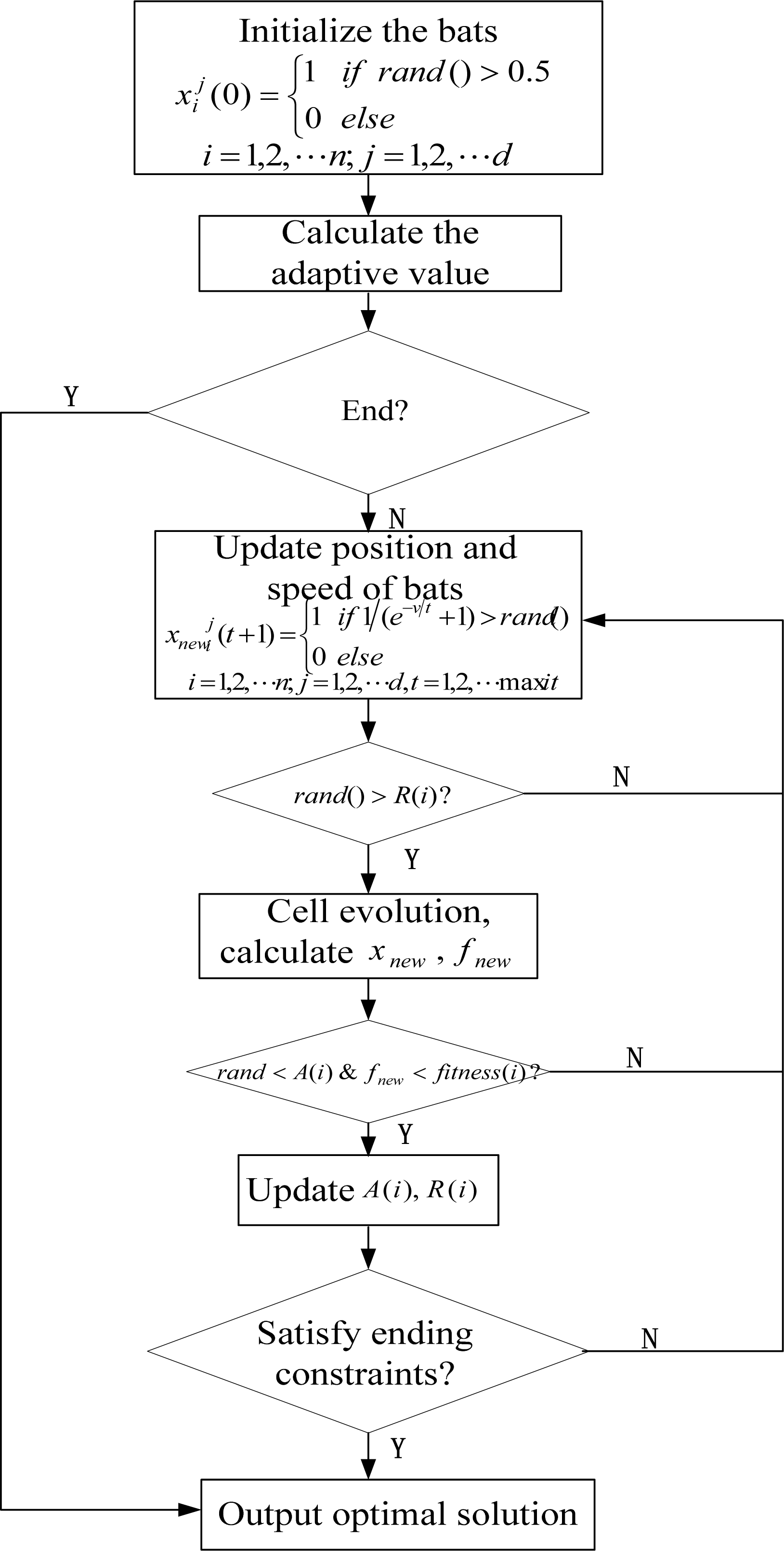
The flow chat of ICBA is illustrated above. In Figure 1, $x_i^j$ is the position of i th bat at j-dimensional space; f_new is the new fitness value; fitness(i) is the optimal fitness value at present; ${x_{\mathit{new}}}_i^j$ is the new position of i th bat at j-dimensional space; V is the speed the bats, maxit is maximum iteration numbers.

5. Case Study and Results

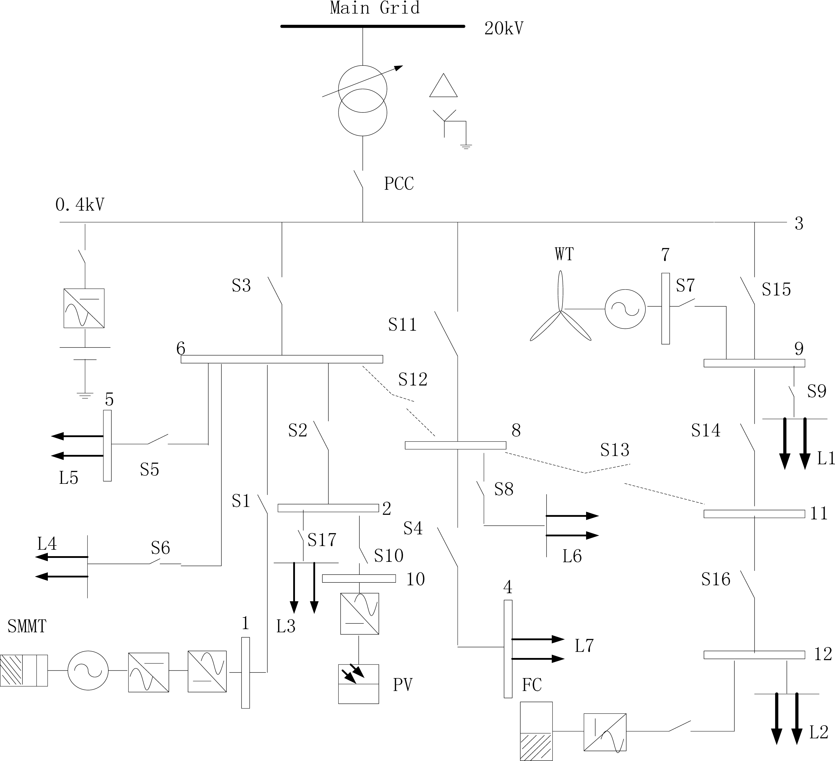
CERTS system published below in literature has been used to demonstrate the effectiveness of the proposed method. In the simulation, scenarios in winter and summer are considered to analyze the microgrid reconfiguration, respectively. The line and load data of CERTS system are taken from [36], and load 1 and 2 are sensitive loads in Figure 2. The structure parameters are shown in

Table 1. Structure parameters.

Bus	4	16	10	12	18
Betweenness	18	51	113	35	18
Bus	15	1	11	5	3
Betweenness	102	18	65	99	18
Feeder	10–15	10–11	5–10	4–15	15–16
Betweenness	84	60	84	18	48
Feeder	15–18	11–12	1–5	16–3
Betweenness	18	34	18	18

.

In addition, several assumptions are listed below:

(1)

The microgrid is connected to the large power grid at first, that means S_PCC = 1;

(2)

The large power grid transmits power energy to the microgrid;

(3)

Microgrid must switch to the islanded mode once the voltage of sensitive loads is less than 0.98 in per-unit value;

(4)

Frequency deviation should be controlled between− 0.1 Hz – 0.1 Hz.

(5)

The DC/AC inverters and DC/DC converters are modeled as an impendence which is sufficient to calculate steady-state operating point in the microgrid.

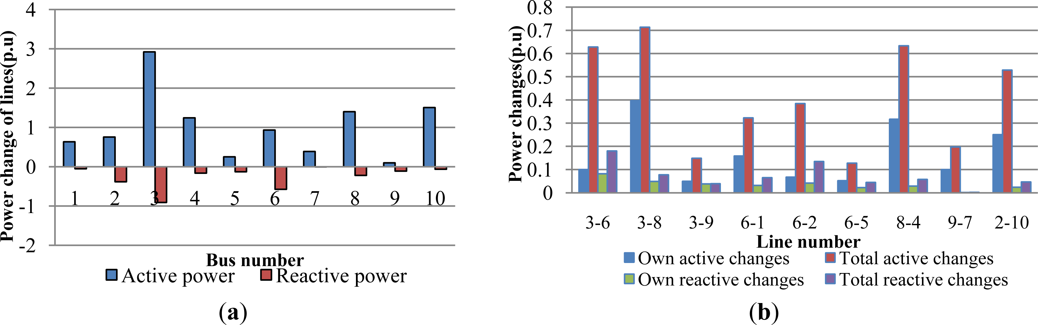
The total voltage deviation caused by each node is shown in Figure 3. It is observed from Figure 3, the voltage deviation (in p.u) caused by node 3 and node 6 is higher, especially node 3, nearly 10. Figure 4 depicts the power flow variation caused by nodes and lines. In Figure 4, the active power variation caused by node 3, 8, 10 is greater, and node 3 and node 6 cause heavy reactive power changes. In the process of line vulnerability assessment, line 3–8 and 8–4 has caused more active power changes, and line 3–6 and 2–6 has caused more reactive power changes in Figure 4 shown on the right. The reactive power impact is not the same as the active, which shows the necessity to take the reactive power into account in vulnerability assessment.

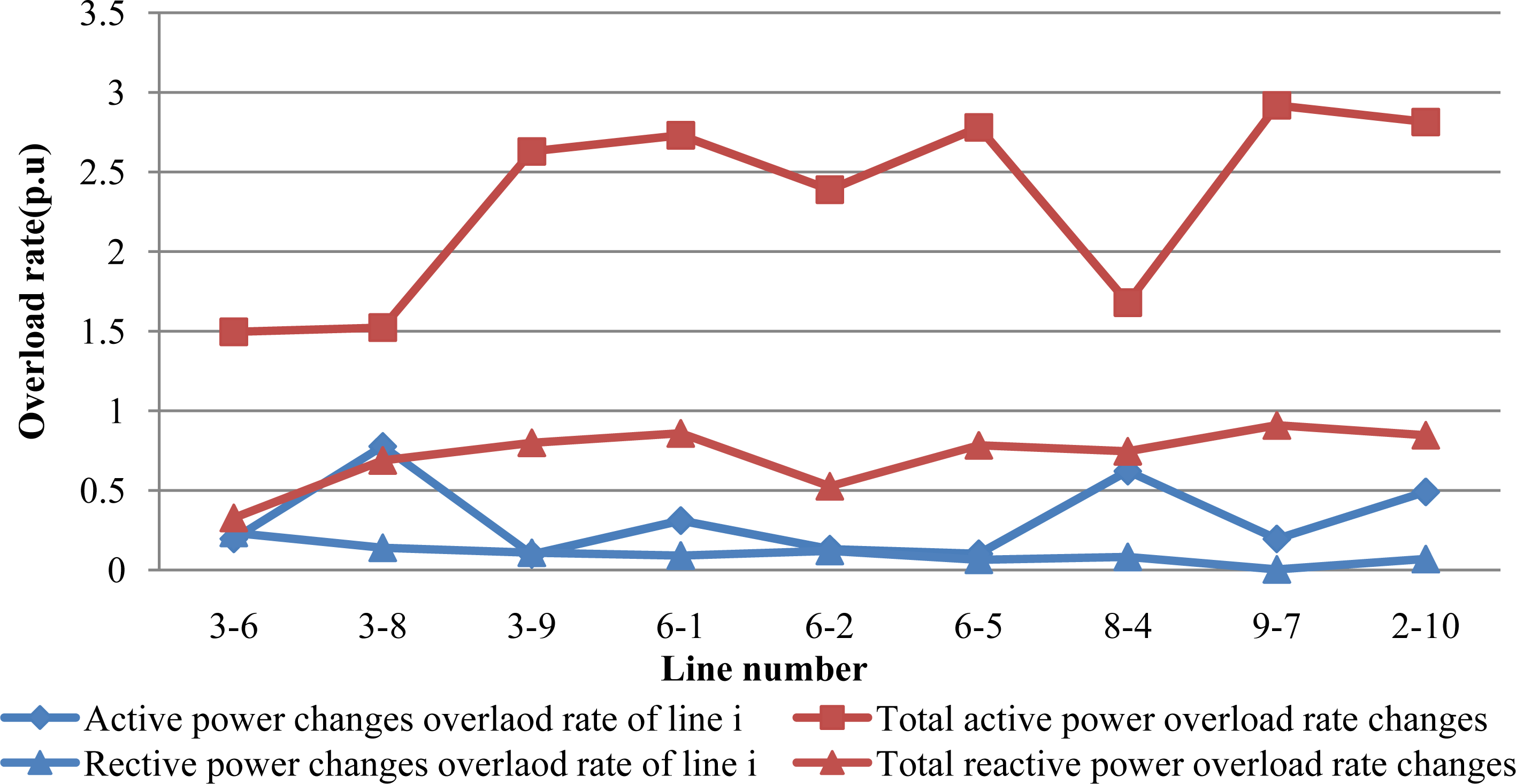
From Figure 5, it is seen that the influence of active power overload rate of line is more serious than reactive power. The total active power overload rate of line 9-7 is the highest, however, the heaviest line of total reactive power overload rate is line 3–8, implying that these lines are overload more easily. The entropy of nodes and lines are given in Figure 6. According to the Equation (7), the total vulnerability value of the microgrid is described in

Table 2. Vulnerability of microgrid (per-unit value: 10⁻²).

Bus	Vulnerability				Feeder	Vulnerability
	This paper	[1]	[4]	[37]		This paper	[1]	[4]	[37]
1	133.578	0.82	1.320	22.794	3–6	288.261	3.57	12.117	247.909
2	312.353	1.25	5.035	51.449	3–8	224.477	2.72	9.457	36.331
3	913.312	3.86	15.132	199.490	3–9	502.217	3.92	18.030	49.620
4	267.864	1.17	4.720	20.419	6-1	102.149	2.02	2.891	8.682
5	143.212	1.30	3.901	49.563	6-2	253.637	3.61	11.982	88.456
6	681.125	2.83	8.772	129.569	6-5	98.322	2.13	2.314	9.912
7	137.503	0.66	1.543	16.240	8-4	128.182	2.30	4.540	8.895
8	395.565	1.63	8.421	34.193	9-7	116.427	2.42	7.201	6.162
9	577.053	3.11	10.187	98.568	2–10	103.763	2.27	3.889	4.175
10	133.021	0.50	1.113	18.652	9–11	151.022	2.76	9.782	28.405
11	138.027	0.98	2.891	51.111	11–12	251.667	2.87	10.031	128.395
12	401.22	2.89	8.273	124.292

.

From Table 2, the main power transmission lines are more vulnerable, and have a serious impact on the microgrid operation. The vulnerability value of sensitive loads (L1, L2) is higher than other load buses, which reflects the main feature of a microgrid—the voltage quality and the power energy transmission management. In addition, several different methods presented in some reference have been used to compare the performance of the method proposed in this paper. The results verify the correctness of the proposed method in this paper.

MOLR is introduced to optimal the microgrid once the system vulnerability is high than the limited value based on the real time load forecasting and power flow state. The load curve from 0:00 am to 8:30am in winter and summer is shown in Figure 7. The ICBA algorithm parameters are listed in

Table 3. Parameters of ICBA.

Fmax	Fmin	A	R	Vmin	Vmax
2	0	0.4	0.8	−4	4

.

From

Table 4. Analysis of on-line reconfiguration.

	Time	Load(kW)	Initial ISV	Reconfiguration	SPCC	Si	ISV after reconfiguration
Summer	9:00	677.062	31.72	No	1	/	/		/
	9:15	691.671	32.18	No	1	/	/		/
	9:30	707.455	33.21	No	1	/	/		/
	9:45	710.482	33.89	No	1	/	/		/
	10:00	717.104	35.47	Yes	0	S3, S4, S12, S13,S15	34.52	37.46	34.52
	10:15	721.239	34.91	No	1	/	/		/
	10:30	723.774	35.18	No	1	/	/		/
	10:45	723.423	35.16	No	1	/	/		/
	11:00	731.887	35.88	No	0	/	/		/
Winter	9:00	634.090	20.12	No	1	/	/		/
	9:15	640.329	22.05	No	1	/	/		/
	9:30	649.895	22.87	No	0	/	/		/
	9:45	656.914	24.91	Yes	0	S3, S8, S12, S16	23.28	23.28	23.28
	10:00	665.758	24.68	No	1	/	/		/
	10:15	671.506	24.98	No	1	/	/		/
	10:30	670.016	25.43	No	1	/	/		/
	10:45	678.267	27.19	Yes	1	S13, S15 L5 = 0.192	26.55	29.23	26.89
	11:00	683.944	26.88	No	1	/	/		/

, MOLR is performed every fifteen minutes based on the real-time load forecasting results from 9:00 am to 11:00 am. At 10:00 am, the current microgrid vulnerable value has exceeded the allowable value. The operators reconfigure the microgrid immediately by switching to islanded mode, opening S12, S13, closing S3, S15, and shedding load 7. If stable, the microgrid will connect to the large power grid again. However, at 11:00 am, the voltage quality of sensitive loads is reduced. According to the operation specification, the microgrid needs to operate in islanded mode, but not change the state of tie and sectionalizing switches.

It has also been observed in Table 4 that the microgrid is reconfigured in islanded mode at 9:45 am in winter, and implements MOLR again at 10:45 am in winter in the grid-connected mode by keeping S_PCC=1. MOLR has demonstrated superiority over the traditional reconfiguration methods.

The entropy and vulnerability index curves are illustrated from Figures 8–9, which is able to describe the trend to help understand the system operation mechanism by 3-dimensional curves. Figure 8 shows the entropy changes caused by nodes and lines to help judge the importance of each unit of microgrid. In Figure 9, the VI₁ curve is changing gently. Once the entropy is close to zero, the VI₁ of nodes increases rapidly. In addition, the VI₂ is mainly determined by the overload rate of lines, increasing with the gradual increase of the overload rate.

Figure 10 shows that the ICBA with a small number of calculations has been able to get the best solution with good accuracy compared with the genetic algorithm (GA) and particle swarm optimization (PSO) algorithm. The method proposed in this paper has avoided the problem of local convergence to provide a strong technical support to the research in the future.

6. Conclusions

Considering the static structure and dynamic operation characteristic of the microgrid, this paper has proposed the application of weighted entropy theory in vulnerability assessment indexes of microgrids based on complex networks theory. The mathematical model of MOLR is established aiming at a minimal vulnerability value. The cell bat algorithm and control strategy are used to ensure the MOLR operation. The results show that the new approach of vulnerability assessment model based on weighted entropy theory is able to describe the total system vulnerability from the aspects of static structure and dynamic operation state of a microgrid to avoid the one-sidedness of the conventional vulnerability assessment methods. The results show that MOLR proposed in this paper is a real-time dynamic simulation based on very short-term load forecasting to guide the operators whether to reconfigure at the next moment, which is different from the previous problem using static methods. The novel method can help dispatch and control accurately on the basis of theory and practice. The results show that improved cellular bat algorithm is able to obtain the optimal solution of reconfiguration problem quickly, and avoid the problem of local convergence like traditional intelligent algorithms.

References

- Yu, X.; Singh, C. A practical approach for integrated power system vulnerability analysis with protection failures. IEEE Trans. Power Syst 2004, 19, 1811–1820. [Google Scholar]
- Wang, X.D. Study of the Evaluation of the Vulnerability of the Grid Based on EEAC Method. Master’s Thesis, North China Electric Power University, Beijing, China. 2004. [Google Scholar]
- Chen, W.; Jiang, Q.; Cao, Y.; Han, Z. Risk-based vulnerability assessment in complex power systems. Power Syst. Technol 2005, 4, 12–17. [Google Scholar]
- Wang, A.; Luo, Y.; Tu, G.; Liu, P. Vulnerability assessment scheme for power system transmission networks based on the fault chain theory. IEEE Trans. Power Syst 2011, 26, 442–450. [Google Scholar]
- Li, Y.; Liu, J.; Liu, X.; Jiang, L.; Xu, W. Vulnerability assessment in power grid cascading failure based on entropy of power flow. Autom. Electr. Power Syst 2012, 36, 1–6. [Google Scholar]
- Sun, K. Research of Complex Network Theory Applied in the Electricity Network. Ph.D’s Thesis, Zhejiang University, Zhejiang, China. 2008. [Google Scholar]
- Zin, A.A.M.; Ferdavani, A.K.; Khairuddin, A.B.; Naeini, M.M. Reconfiguration of radial electrical distribution network through minimum-current circular-updating-mechanism method. IEEE Trans. Power Syst 2012, 27, 968–974. [Google Scholar]
- Gonzalez, A.; Echavarren, F.M.; Rouco, L.; Gomez, T.A. Sensitivities computation method for reconfiguration of radial networks. IEEE Trans. Power Syst 2012, 27, 1–8. [Google Scholar]
- Rao, R.S.; Ravindra, K.; Satish, K.; Narasimham, S.V.L. Power loss minimization in distribution system using network reconfiguration in the presence of distributed generation. IEEE Trans. Power Syst 2013, 28, 1–9. [Google Scholar]
- Zin, A.A.M.; Ferdavani, A.K.; Bin Khairuddin, A.; Naeini, M.M. Two circular-updating hybrid heuristic methods for minimum-loss reconfiguration of electrical distribution network. IEEE Trans. Power Syst 2013, 28, 1318–1323. [Google Scholar]
- Zhao, D.; Liu, Y.; Zhou, W.; Si, Z.; Xia, D. Distribution network reconfiguration to reduce energy loss. J. Xi’an Jiao.Tong Univ 1999, 33, 16–19. [Google Scholar]
- Wang, S.; Wang, C. Distribution network reconfiguration based on interval algorithm to maximize confidence of energy loss reduction. Autom. Electr. Power Syst 2001, 12, 27–32. [Google Scholar]
- Srinivasa Rao, R.; Narasimham, S.V.L.; Ramalinga Raju, M.; Srinivasa Rao, A. Optimal network reconfiguration of large-scale distribution system using harmony search algorithm. IEEE Trans. Power Syst 2011, 26, 1080–1088. [Google Scholar]
- Liu, L.; Chen, X. Reconfiguration of distribution networks based on fuzzy algorithm. Proc. Chin. Soc. Electr. Eng 2000, 20, 66–69. [Google Scholar]
- Malekpour, A.R.; Niknam, T.; Pahwa, A.; Fard, A.K. Multi-objective stochastic distribution feeder reconfiguration in systems with wind power generators and fuel cells using the point estimate method. IEEE Trans. Power Syst 2013, 28, 1483–1492. [Google Scholar]
- Wu, W.-C.; Tsai, M.-S. Application of enhanced integer coded particle swarm optimization for distribution system feeder reconfiguration. IEEE Trans. Power Syst 2011, 26, 1591–1599. [Google Scholar]
- Yu, Q.; Solanki, J.; Padmati, K.; Kumar, N.; Srivastava, A.K.; Bastos, J.; Schulz, N.N. Intelligent methods for reconfiguration of terrestrial and shipboard power systems. Proceedings of the IEEE Power and Energy Society General Meeting, Pittsburgh, PA, USA, 20–24 July 2008.
- Li, Z.; Chen, X.; Yu, K.; Sun, Y.; Liu, H. A hybrid particle swarm optimization approach for distribution network reconfiguration problem. In Proceedings of the IEEE Power and Energy Society General Meeting, Pittsburgh, PA, USA, 20–24 July 2008.
- Ahuja, A.; Das, S.; Pahwa, A. An AIS-ACO hybrid approach for multi-objective distribution system reconfiguration. IEEE Trans. Power Syst 2007, 22, 1101–1111. [Google Scholar]
- Luan, W.P.; Irving, M.R.; Daniel, J.S. Genetic algorithm for supply restoration and optimal load shedding in power system distribution networks. IEE Proc. Generat. Transm. Distrib 2002, 149, 145–151. [Google Scholar]
- Meek, C.D. Investigation of optimization methods used for reconfiguration of the naval electric ship power system; M. S. thesis, University of Texas, Austin, USA; 2004. [Google Scholar]
- Crucitti, P.; Latora, V.; Marchiori, M. Model for cascading failures in complex networks. Phys. Rev. E 2004, 69, 045104. [Google Scholar]
- Alvert, R.; Albert, I.; Nakarado, G.L. Structural vulnerability of the North American power grid. Phys. Rev. E 2004, 69, 025103. [Google Scholar]
- Rosas-Casals, M.; Valverde, S.; Sole, R.V. Topological vulnerability of the European power grid under errors and attacks. Int. J. Bifurcation Chaos 2007, 17, 2465–2475. [Google Scholar]
- Ten, C.; Lui, C.; Manimaran, G. Vulnerability assessment of cyber-security for SCADA systems. IEEE Trans. Power Syst 2008, 23, 1836–1846. [Google Scholar]
- Brandwajn, V.; Kumar, A.B.R.; Ipakchi, A.; Bose, A.; Kuo, S.D. Severity indices for contingency screening in dynamic security assessment. IEEE Trans. Power Syst 1997, 12, 1136–1142. [Google Scholar]
- Zhou, R.; Liu, S.; W. Survey of applications of entropy in decision analysis. Control. Dec 2008, 23, 361–367. [Google Scholar]
- Chen, T.Y.; Li, C.H. Determining objective weights with intuitionistic fuzzy entropy measures: a comparative analysis. Inform. Sci 2010, 180, 4207–4222. [Google Scholar]
- Zhang, X. Entropy weight theory-based integrated evaluation model of natural disasters. J. Nat. Dis 2009, 18, 189–192. [Google Scholar]
- Khoa, T.Q.D.; Phan, B.T.T. Ant colony search based loss minimumfor reconfiguration of distribution systems. In Proceedings of the IEEE Power India Conference, New Delhi, India, 10–12 April 2006.
- Esmin, A.A.A.; Lambert-Torres, G.; de Souza, A.C.Z. A hybrid particle swarm optimization applied to loss power minimization. IEEE Trans. Power Syst 2005, 20, 859–866. [Google Scholar]
- Wu, W.-C.; Tsai, M.-S. Feeder reconfiguration using binary coding particle swarm optimization. Int. J. Control Autom. Syst 2008, 6, 488–494. [Google Scholar]
- Farahani, V.; Vahidi, B.; Abyaneh, H.A. Reconfiguration and capacitor placement simultaneously for energy loss reduction based on an improved reconfiguration method. IEEE Trans. Power Syst 2012, 27, 587–595. [Google Scholar]
- Buriol, L.; Franca, P.; Moscato, P. A new memetic algorithm for the asymmetric traveling salesman problem. J. Heuristics 2004, 10, 483–506. [Google Scholar]
- Bora, T.C.; Coelho, L.D.S; Lebensztajn, L. Bat-inspired optimization approach for the brushless dc wheel motor problem. IEEE Trans.Magn 2012, 48, 947–950. [Google Scholar]
- Qiao, Y.; Lu, Z.; Mei, S. Microgrid Reconfiguration in Catastrop Failure of Large Power Systems. Proceedings of the International Conference on Sustainable Power Generation and Supply, Nanjing, China, 6–7 April 2009.
- Mahadev, P.M.; Christie, R.D. Envisioning power system data: Vulnerability and severity representations for static security assessment. IEEE Trans. Power Syst 1994, 9, 1915–1920. [Google Scholar]