Realization of Thermal Inertia in Frequency Domain

Abstract

To realize the lagging behavior in heat conduction observed in these two decades, this paper firstly theoretically excludes the possibility that the underlying thermal inertia is a result of the time delay in heat diffusion. Instead, we verify in experiments the electro-thermal analogy, wherein the thermal inertial is parameterized by thermal inductance that formulates hyperbolic heat-conduction. The thermal hyperbolicity exhibits a special frequency response in Bode plot, wherein the amplitude ratios is kept flat after crossing some certain frequency, as opposed to Fourier heat-conduction. We apply this specialty to design an instrument that reliably identifies thermal inductances of some materials in frequency domain. The instrument is embedded with a DSP-based frequency synthesizer capable of modulating frequencies in utmost high-resolution. Thermal inertia implies a new possibility for energy storage in analogy to inductive energy storage in electricity or mechanics.

1. Introduction

Thermal inertia in heat transfer was observed in the lab or in practice during the past decades. As early as 1946, Bosworth postulated his experimental observation on the principles of electrothermal analogy, wherein the electric inductance has a thermal analogy in heat transfer [1,2]. In the last decade of the twentieth century, Kaminski and Vedavarz et al. tabulated the relaxation times of heat conduction in metals, superconductors, semiconductors, organic materials and porous materials [3–5]. In 2003, Roetzel et al. made another table for sand, NaHCO₃ and meat [6]. Between these two quantitative measurements, in 1995, Mitra et al. found the conduction of heat in processed meat to be propagated like a wave, providing evidence that heat-transfer dynamics are hyperbolic [7]. In 2002, Jiang et al. applied laser pulses to excite apparent non-Fourier phenomena in porous materials of small-scale dimensions [8]. Sousa et al. claimed that the theory of hyperbolic heat transfer in agar gel improves the accuracy of radiofrequency ablation models and procedures [9]. Currently, thermal inertia seriously affects nano-scaled or bio- heat treatments, say, in [10–12]. The thermal inertia under these investigations has been mathematically modeled by time-delay in heat diffusion or thermal inductance with an electro-thermal analogy.

In fact, thermal-inductance modeling can be traced back to one century to when Maxwell [13] and Nernst [14] suggested through theoretical observations that, in properly chosen conductors, at low temperatures, heat may have sufficient inertia for oscillatory discharge to happen. In 1944, Peshkov measured the propagation velocity of heat flux in liquid helium at 1.4 K to be 19 m/s [15], which contradicts Fourier’s law of heat conduction. Taitel hypothesized that the transient temperature at the middle location of a slab with constant-temperature heat source at two ends can be higher than that of the sources, a phenomenon which is called Taitel’s paradox [16].

Along with those experimental observations mentioned above there are a number of numerical studies [17–22], wherein first-order approximation of time-delayed modeling results in thermal-inductance modeling. Therefore, it is hard to distinguish thermal-inductance modeling from time-delay modeling merely based on computer simulation. On the other hand, these numerical responses matching experimental observations indirectly support the physical realization of thermal inertia by thermal inductance. Firstly in this paper, we will give a theoretical proof that the physical realization of thermal inertia by time-delayed diffusion contradicts the first law of thermodynamics.

Although these two realizations can have indistinguishable responses of temperature or heat-flux in computer modeling, only the thermal-inductance realization involves the following aspects of physical significances:

(1)

There is a new “storage-form” since energy is stored in an inductive element though which a current of entropy flows;

(2)

Thermal inductance dominates the performance of high-speed thermal processes, such as the heating by short-time laser pulses, and

(3)

Even with small temperature differences, large energies can still be pumped in the form of heat-flux into the material, provided that we find how to increase its thermal inductance.

The literature documents three aspects of non-Fourier phenomena in heat transfer, which stimulated our efforts to understand more about thermal inertia:

• (nF1) The temperature at some locations of heat-conduction materials subjected to a constant temperature heat source can be higher than that of the source during the transience of heat transfer, which implies that heat flux can flow from the lower temperature level to a higher level;

• (nF2) A temperature gradient pulse induces temperature vibrations at fixed locations, in which temperature ought to wave-propagate before internal energy is exhausted, and

• (nF3) At any location of a heat-conduction material, an abrupt change of temperature will not result in an abrupt change of heat flux- some time lags have been observed, from which we infer that the speed of heat-transfer is comparatively smaller than that of Fourier’s prediction.

For these non-Fourier phenomena, Cattaneo [23,24] and Vernotte [25,26] proposed to replace the zero-order diffusion equation with the first-order equation:

$$\mathit{q}+\tau \partial \mathit{q}/\partial t=-k\nabla T\hspace{0.17em}\hspace{0.17em}\hspace{0.17em}\hspace{0.17em}\hspace{0.17em}\hspace{0.17em}\hspace{0.17em}(\text{CV-Equation})$$

(1)

where T and q stand for temperature and heat-flux, respectively, and τ indicates the observed time-lag. Coupling the CV-Equation to thermal capacitance yields a hyperbolic equation, which can capture the phenomena described in nF1, nF2 and nF3.

However, the CV-Equation seems not in line with the Clausius formulation of the second law of thermodynamics, since the heat-flux is allowed to flow into higher-temperature regions from a lower-temperature region in the transient state. The mainstream thus acknowledged that the CV-Equation ought to be a first-order approximation of the time-delayed heat-diffusion equation:

$$\mathit{q}(x,t+\tau )=-k\nabla T(x,t)\hspace{0.17em}\hspace{0.17em}\hspace{0.17em}\hspace{0.17em}\hspace{0.17em}\hspace{0.17em}\hspace{0.17em}(\text{TD-Equation})$$

(2)

which apparently still complies with the Clausius formulation. Coupling the TD-Equation to thermal capacitance, on the other hand, yields a parabolic equation with time-delayed Laplacian (TDP-Equation).

Unfortunately, we will perform a bifurcation analysis to show that the TDP-Equation is ill-posed, that is, given any initial condition, none of (bounded) solutions exist, no matter how small the time-delay τ is. Specifically, accompanied by the ill-posed dynamics is the fact that even a tiny heat-flux pulse input to the heat-transfer domain insulated from a heat source can trigger the temperature to be unbounded. This contradicts the first law of thermodynamics that excludes the possibility that thermal potential, part of the internal energy, becomes infinite due to a finite energy input to the domain. Thus, the hypothesis of time-delayed heat diffusion is untrue.

The bifurcation analysis adopts the composite of Laplace transform and Galerkin projection: the Laplace-Galerkin transform in space-time [27]. With this newly developed transform, we represent the TDP-Equation by a transfer function served for pure algebra, which is a ratio of polynomials dependent on two variables: one is for space and the other is for time. With the capability of pure algebra, we construct the dynamics as a feedback interconnection of two 2D transfer-functions: one is for thermal capacitance, and the other is for the time-delayed heat diffusion. This makes it possible to extend the Nyquist criterion and Root Locus on stability analyses.

On the other hand, the thermal circuit resulting from the electro-thermo analogy captures the non-Fourier phenomena and can be formulated as a positive-damped, hyperbolic equation, compatible with the passivity of heat conduction. As mentioned, the hyperbolic nature of heat conduction seems incompatible with the Clausius formulation of the second law of thermodynamics. This incompatibility can be remedied by the inclusion of the thermal kinetics stored in the thermal inductor into the internal energy concept. Such a remedy is supported by the theory-extended irreversible thermodynamics [28,29].

One step further from the theoretical work [30], in this work we perform experimental measurements to prove that thermal inertial can be parameterized by thermal inductance within the electro-thermal analogy. In advance of these designing experiments, it is numerically found that thermal hyperbolicity exhibits a special frequency response, for example, in a Bode plot the amplitude ratios are no longer decreasing after some frequency, as opposed to parabolic Fourier heat-conduction, those of which are monotonically decreasing along with the increase of input frequencies. This frequency-domain specialty is then applied to reliably identify thermal inductances of some materials. In fact, measurements of thermal inertia have been documented in several papers, among which are [7] and [31]. They identified the time delays in heat conduction in the time domain, but we employ the thermal hyperbolicity to reliably discover in the frequency domain the fact that thermal inertia is due to thermal inductance rather than the time-delay. An instrument is made for this purpose that is embedded with a DSP-based frequency synthesizer to obtain high-resolution Bode plot, especially in the concerned low-frequency region, which is beyond the flavors of current frequency generators. Therefore we design a limit-cycle generator and implement it into DSP-engine embedded microcontrollers (DSP-controller) to fulfill this task.

As a limit-cycle generator, the filtered van der Pol oscillator is implemented into a DSP-controller that provides sinusoidal control signals and is capable of modulating frequency in a real-time fashion. Its dynamics is transformed into iterated computation of addition and multiplication performed by the DSP engine inside. This kind of DSP-based implementation [32–34] is in line with the function of the DSP engine that is a master of fast calculation of addition and multiplication of floating numbers. Microcontrollers are really needed in practice for frequency synthesizers, since analog circuits lack communication ports, crystal oscillators have no reliable low-frequency outputs, and general-purpose computers transport signals to peripheral devices very slowly. Furthermore, DSP-based linear oscillators are not candidates, since they produce in the long run no sustained oscillations.

For the time being, there are two popular frequency synthesizers in industry: one is by data scheduling [35] and the other is by online sinusoidal function [36,37], both of which are widely used in wireless communication. In the data scheduling type, the working chip stores a table of data in code space that digitally shape a sinusoidal function. The targeted frequency is determined by the number of times the whole table is fetched per second at a fixed instruction clock, which is adjustable by the number of entries to be fetched in the entire table. This requires a large ROM size for long tables and produces wide frequency-span for radio modulation. Such ROM size is usually unavailable in DSP-controllers, and building special ICs for this purpose prevails [38–41]. One characteristic of data scheduling for frequency synthesizers is low frequency-resolution, since the number of entries being fetched is always an integer. This situation is worse at lower frequency-range. It prevents this method from being applied to perform system identification of heat conduction in frequency domain. On the other hand, with the limit-cycle approach as developed by this paper, the frequency resolution can be pushed to the maximum allowed by hardware, which is usually more than 16 megabytes.

In the type of on-line sinusoidal function, the working chip has to compute sinusoidal functions one time within each sampling period, wherein the sinusoidal function is approximated by Taylor-series expansion [37] or by other complex algebra. Such a high computational burden is beyond the capability of DSP-controllers, and often requires FPGA chips. However, we really need DSP-controllers for system identification, since not just the frequency synthesizer is in the chip, but also an on-line window Fourier transform, and color and white noises filters to remove sensing contamination. All of these modules are implemented through DSP-based implementation. Otherwise, a special IC or a single-task FPGA cannot be integrated into other modules to fulfill control purposes. Moreover, there is usually a variety of peripherals in DSP-controllers served for control purposes. For example, almost every Microchip dsPIC has analog-to-digital (A/D) and pulse-width modulation (PWM) peripherals, for inputting analog signals from sensors and outputting PWM signals to switching power converters.

2. 2D Transfer Function

This section briefs the mathematical tool named by 2D Transfer Function, which will appear in the remaining sections.

Consider a class of Laplacian operators 𝒶 = −β∇² (β > 0) defined over the set of spatial functions:

$$D(\mathbf{𝒶})=\left\{\psi :\psi \in L_2(\Omega ),\hspace{0.17em}\hspace{0.17em}\psi (x)=0\hspace{0.17em}\hspace{0.17em}\text{or}\hspace{0.17em}\hspace{0.17em}\nabla \psi (x)=0\hspace{0.17em}\hspace{0.17em}\hspace{0.17em}\text{at}\hspace{0.17em}\hspace{0.17em}x\in \partial \Omega \right\}$$

(3)

where Ω ⊂ ℜ³ is a bounded domain. Based on the Sturm-Liouville theory [42], such an operator 𝒶 is nonnegative-definite and self-adjoint, which implies that all of its eigenvalues are nonnegative real numbers, and its normalized eigenfunctions constitute an orthonormal, complete basis of L₂ (Ω). Denote its countable set of eigenvalues by Λ and the eigenfunction associated with λ ∈ Λ by ϕ(λ, x), i.e.,

$$\mathbf{𝒶}\varphi (\lambda ,x)=\lambda \varphi (\lambda ,x),\hspace{0.17em}\hspace{0.17em}\varphi \in D(\mathbf{𝒶})$$

(4)

The Galerkin transform $𝒢$, F(λ) = $𝒢$[f(x)], from spatial functions to modal functions is defined by:

$$F(\lambda )\equiv {\int }_{\Omega }\varphi (\lambda ,x)f(x)dx$$

(5)

Completeness and orthonormality of the eigenfunctions basis imply that the Galerkin transform $𝒢$ has a unique inverse $𝒢$⁻¹, f(x) = $𝒢$⁻¹[F(λ)]:

$$\mathbf{\mathscr{H}}=\mathbf{ℒ}\mathbf{𝒢}=\mathbf{𝒢}\mathbf{ℒ}$$

(6)

which is the composite of the Galerkin transform and the Laplace transform, and explicitly:

$$F(\lambda ,s)\equiv \mathbf{\mathscr{H}}[f(x,t)]={\int }_{0^{-}}^{\infty }{\int }_{\Omega }{e}^{-st}\varphi (\lambda ,x)f(x,t)\mathit{dxdt}$$

(7)

Accordingly, the inverse Laplace-Galerkin transform is the composite of the inverse Laplace transform and the inverse Galerkin transform, that is:

$${\mathbf{\mathscr{H}}}^{-1}={\mathbf{𝒢}}^{-1}{\mathbf{ℒ}}^{-1}={\mathbf{ℒ}}^{-1}{\mathbf{𝒢}}^{-1}$$

(8)

and explicitly:

$$f(x,t)\equiv {\mathbf{\mathscr{H}}}^{-1}[F(\lambda ,s)]=\frac{1}{2\pi j}\sum _{\lambda \in \Lambda }{\oint }_{C}F(\lambda ,s)\varphi (\lambda ,x)e^{ts}ds$$

(9)

where C is a closed contour that encircles poles of F(λ, s) for all λ ∈ Λ.

Basic properties of the Galerkin and Laplace transforms are, respectively,

$$\mathbf{𝒢}[\mathbf{𝒶}f(x,t)]=\lambda \mathbf{𝒢}[f(x,t)]$$

(10)

and:

$$\mathbf{ℒ}[{\mathbf{𝒟}}_{t}f(x,t)]=s\mathbf{ℒ}[f(x,t)]$$

(11)

for zero initial conditions at t = 0⁻, where $𝒟$_t denotes temporal differentiation. Combining these two properties, the Laplace-Galerkin transform $\mathscr{H}$ is of:

$$\mathbf{\mathscr{H}}[h({\mathbf{𝒟}}_t,\mathbf{𝒶})f(x,t)]=\beta (s,\lambda )\cdot \mathbf{\mathscr{H}}[f(x,t)]$$

(12)

where h is a ratio of two expressions of finite or some infinite length constructed from two independent variables, one standing for space and the other for time, allowing for the operations of addition, subtraction, multiplication, integer exponents in time, and fraction-order exponents in space. For example:

$$\mathbf{\mathscr{H}}\left[\frac{{\mathbf{𝒟}}_t-{\mathbf{𝒶}}^{1/2}}{{\mathbf{𝒟}}_t+{\mathbf{𝒶}}^{1/2}}f(x,t)\right]=\frac{s-\sqrt{\lambda }}{s+\sqrt{\lambda }}F(\lambda ,s)$$

(13)

Linear dynamics Ĝ governed by partial differential equation ψ = Ĝu with a spatial Sturm-Liouville operator has uniquely a functional representation: Ψ(λ, s) = G(λ, s)U(λ, s) [27]. The modal-complex function G is defined as the 2D transfer-function of the dynamics Ĝ. This is obtained by taking Laplace-Galerkin transform $\mathscr{H}$ on both sides of ψ = Ĝu, where u stands for the input spatial-temporal function with U(λ, s) = $\mathscr{H}$[u (x, t)] and ψ for the output spatial-temporal function with Ψ(λ, s) = $\mathscr{H}$[ψ(x, t)].

Take as an explanatory example the longitudinal wave dynamics Ĝ :

$$\frac{{\partial }^2\psi }{\partial t^2}-\frac{{\partial }^2\psi }{\partial x^2}=u,\hspace{0.17em}\hspace{0.17em}\hspace{0.17em}\hspace{0.17em}0\le x\le \pi ,\hspace{0.17em}\hspace{0.17em}\hspace{0.17em}\hspace{0.17em}\hspace{0.17em}\hspace{0.17em}0\le t<\infty$$

(14)

$$\psi (0,t)=0,\hspace{0.17em}\hspace{0.17em}\hspace{0.17em}\hspace{0.17em}\psi (\pi ,t)=0,\hspace{0.17em}\hspace{0.17em}\hspace{0.17em}\hspace{0.17em}\hspace{0.17em}0\le t<\infty$$

(15)

We firstly check that the negative Laplacian −∂²/∂x² is of eigenvalues Λ = {1,4,9,…} associated with eigenfunctions $\varphi (\lambda ,x)=\sqrt{2/\pi }\text{sin}\sqrt{\lambda }x$. Taking Laplace-Galerkin transform $\mathscr{H}$ on both sides of the differential equation yields:

$$(s^2+\lambda )\Psi (\lambda ,s)=U(\lambda ,s),\hspace{0.17em}\hspace{0.17em}\hspace{0.17em}\hspace{0.17em}\hspace{0.17em}\hspace{0.17em}\text{or}\hspace{0.17em}\hspace{0.17em}\hspace{0.17em}\hspace{0.17em}\hspace{0.17em}\hspace{0.17em}\Psi (\lambda ,s)=\frac{1}{s^2+\lambda }U(\lambda ,s)$$

(16)

That is, the 2D transfer function of the dynamics Ĝ is:

$$G(\lambda ,s)\equiv \frac{\Psi (\lambda ,s)}{U(\lambda ,s)}=\frac{1}{s^2+\lambda }$$

(17)

As the input u is $u(x,t)=\delta (t)\sum _{n=1}^{\infty }{\varphi }_n(x)$ that is the spatial-temporal unit-pulse since its Laplace-Galerkin transform is one, the corresponding output defines the impulse response g of the dynamics Ĝ. Taking the inverse Laplace-Galerkin transform of the 2D transfer function G yields the impulse response:

$$g(x,t)=\sum _{p=1}^{\infty }\sqrt{2/\pi }\text{sin}\hspace{0.17em}px\cdot {\mathbf{ℒ}}^{-1}\left(\frac{1}{s^2+p^2}\right)=\sum _{p=1}^{\infty }\frac{\sqrt{2}}{p\sqrt{\pi }}\text{sin}\hspace{0.17em}px\text{sin}\hspace{0.17em}pt$$

(18)

To verify this solution, let us integrate the differential equation from t = 0⁻ to t = 0⁺ to yield the initial condition: ψ(x,0) = 0 and $\frac{\partial \psi }{\partial t}(x,0)=\sum _{n=1}^{\infty }{\varphi }_n(x)$ at t = 0⁺. Thereby, the impulse response becomes the solution of the following homogeneous differential equation:

$$\frac{{\partial }^2\psi }{\partial t^2}-\frac{{\partial }^2\psi }{\partial x^2}=0$$

(19)

$$\psi (0,t)=0,\hspace{0.17em}\hspace{0.17em}\hspace{0.17em}\psi (\pi ,t)=0$$

(20)

$$\psi (x,0)=0,\hspace{0.17em}\hspace{0.17em}\frac{\partial \psi }{\partial t}(x,0)=\sum _{n=1}^{\infty }{\phi }_n(x)$$

(21)

which can be solved via the conventional Separation-of-Variables method. It is easy to find that both arrive at the same solution.

Representation of partial differential equations by 2D transfer functions renders its stability analysis to be in essence the same as 1D stability analysis. For example:

(1)

For a 2D transfer function:

$$G(\lambda ,s)\equiv \frac{N(\lambda ,s)}{M(\lambda ,s)}$$

(22)

where M and N are polynomials of s and allows for fraction-orders of λ, the set:

$$P=\{s:M(\lambda ,s)=0,\hspace{0.17em}\hspace{0.17em}\forall \lambda \in \Lambda \}$$

(23)

contains all of its poles. Its coherent dynamics Ĝ is asymptotically stable if all poles are on the left-half plane.

(2)

For a dynamics that is represented by feedback-interconnection of G and H that have no poles in the right half-plane the assembly of loop transfer functions is defined by the set L = {G(λ, ·)H(λ, ·): λ ∈ Λ}. Then, this dynamics is unstable if any member of L has its Nyquist plot encircling (−1,0) in the complex plane. The instability means that the output of the loop will grow exponentially up to be unbound even the input is as tiny as infinitesimal.

3. Time-Delay Heat Conduction

Assume that there really exists a time-delay τ in heat diffusion, i.e.,

$$\mathit{q}(x,t+\tau )=-k\nabla T(x,t)$$

(24)

Coupling it with the equation of energy conservation:

$$\rho C_v\frac{\partial T(x,t)}{\partial t}=-\nabla \cdot \mathit{q}(x,t)+Q(x,t)$$

(25)

leads to the time-delayed parabolic equation:

$$\rho C_v\frac{\partial T(x,t)}{\partial t}-k{\nabla }^{2}T(x,t-\tau )=Q(x,t)$$

(26)

over a bounded domain Ω, where Q stands for the heat generation in the interior of Ω. Consider the class of boundary conditions: −k∇T(x) = q₀(x) or T(x) = T₀(x) for x ∈ ∂Ω, where T₀ and q₀ stands for inputs of temperature and heat-flux, respectively, on the boundary ∂Ω.

Denote the equilibrium point of Equation (26) by T̄, i.e.,

$$-k{\nabla }^2\overline{T}(x)=\overline{Q}(x)\hspace{0.17em}\hspace{0.17em}\hspace{0.17em}\hspace{0.17em}\hspace{0.17em}\hspace{0.17em}\text{for}\hspace{0.17em}\hspace{0.17em}\hspace{0.17em}\hspace{0.17em}\hspace{0.17em}x\in \Omega$$

(27)

$$-k\nabla \overline{T}(x)={\mathit{q}}_0(x)\hspace{0.17em}\hspace{0.17em}\hspace{0.17em}\hspace{0.17em}\hspace{0.17em}\hspace{0.17em}\hspace{0.17em}\text{or}\hspace{0.17em}\hspace{0.17em}\hspace{0.17em}\hspace{0.17em}\hspace{0.17em}\hspace{0.17em}\overline{T}(x)=T_0(x)\hspace{0.17em}\hspace{0.17em}\hspace{0.17em}\hspace{0.17em}\hspace{0.17em}\hspace{0.17em}\text{for}\hspace{0.17em}\hspace{0.17em}\hspace{0.17em}\hspace{0.17em}\hspace{0.17em}x\in \partial \Omega$$

(28)

and the perturbation around the equilibrium T̄ by ψ. That is, the temperature T and the heat generation are decomposed, respectively, by:

$$T(x,t)=\overline{T}(x)+\psi (x,t),\hspace{0.17em}\hspace{0.17em}\hspace{0.17em}\hspace{0.17em}x\in \Omega ,\hspace{0.17em}\hspace{0.17em}\hspace{0.17em}\hspace{0.17em}\hspace{0.17em}t\in [0,\infty )$$

(29)

$$Q(x,t)=\overline{Q}(x)+Q^{\prime }(x,t),\hspace{0.17em}\hspace{0.17em}\hspace{0.17em}\hspace{0.17em}\hspace{0.17em}x\in \Omega ,\hspace{0.17em}\hspace{0.17em}\hspace{0.17em}\hspace{0.17em}\hspace{0.17em}t\in [0,\infty )$$

(30)

Note that Equation (26) has only the equilibrium point T̄ that indicates the steady-state temperature observed in Fourier and non-Fourier heat-transfers. Substituting Equations (29) and (30) into Equation (26) yields the equation governing the perturbation dynamics:

$$\rho C_v\frac{\partial \psi (x,t)}{\partial t}-k{\nabla }^2\psi (x,t-\tau )=Q^{\prime }(x,t)$$

(31)

with homogeneous boundary conditions: ∇ψ = 0 or ψ = 0 on ∂Ω. Let Equation (31) be further rewritten as:

$$\frac{\partial \psi (x,t)}{\partial t}-\beta {\nabla }^2\psi (x,t-\tau )=u(x,t);\hspace{0.17em}\hspace{0.17em}\hspace{0.17em}\hspace{0.17em}\nabla \psi =0\hspace{0.17em}\hspace{0.17em}\hspace{0.17em}\hspace{0.17em}\hspace{0.17em}\hspace{0.17em}\hspace{0.17em}\text{or}\hspace{0.17em}\hspace{0.17em}\hspace{0.17em}\hspace{0.17em}\hspace{0.17em}\psi =0\hspace{0.17em}\hspace{0.17em}\hspace{0.17em}\hspace{0.17em}\hspace{0.17em}\text{on}\hspace{0.17em}\hspace{0.17em}\hspace{0.17em}\hspace{0.17em}\partial \Omega$$

(32)

where β = k/ρC_v is a positive number. Equation (32) is one of parabolic equations with time-delayed Laplacian of homogeneous boundary conditions (TDP-Equation).

In this section it will be shown that the TDP-Equation of Equation (12) is unstable, no matter how small the time delay τ is. We will prove this with the 2D transfer-function in Section 2.

As mentioned in Section 2, all eigenvalues λ ’s of the Laplacian operator −β∇² in Equation (32) are nonnegative real, and its eigenfunctions ϕ ’s can constitute an orthonormal, complete basis of L₂ (Ω). Based on Equation (12), the 2D transfer-function of the TDP-Equation in Equation (32) is known as:

$$G(\lambda ,s)=\frac{1}{s+\lambda e^{-\tau s}}$$

(33)

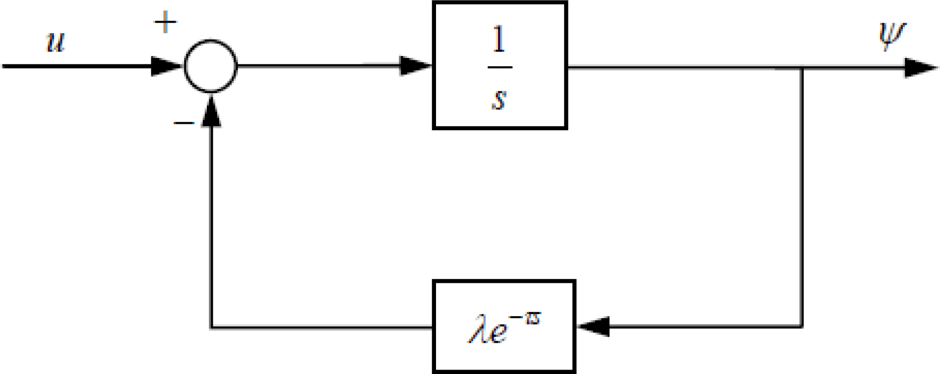
This transfer function can further be represented by the feedback-interconnection of thermal capacitance 1/s and time-delayed heat diffusion λe^−τs, as shown in Figure 1. Nyquist criterion [43] can then be applied to do stability analysis for this loop, as discussed in Section 2. Since the Nyquist plot of e^−τs/s has the gain margin π/2τ, Nyquist plots of the loop-gains λe^−τs/s in Figure 1 will encircle (−1,0) for all λ > π/2τ. There are always existing eigenvalues λ of the Laplacian operator −β∇² that are larger than π/2τ for all delay times τ > 0, so the feedback loop in Figure 1 is unstable. Therefore, we come to the result that the perturbation dynamics of Equation (32) around the unique equilibrium point T̄ is unstable, no matter how small the delay time τ is.

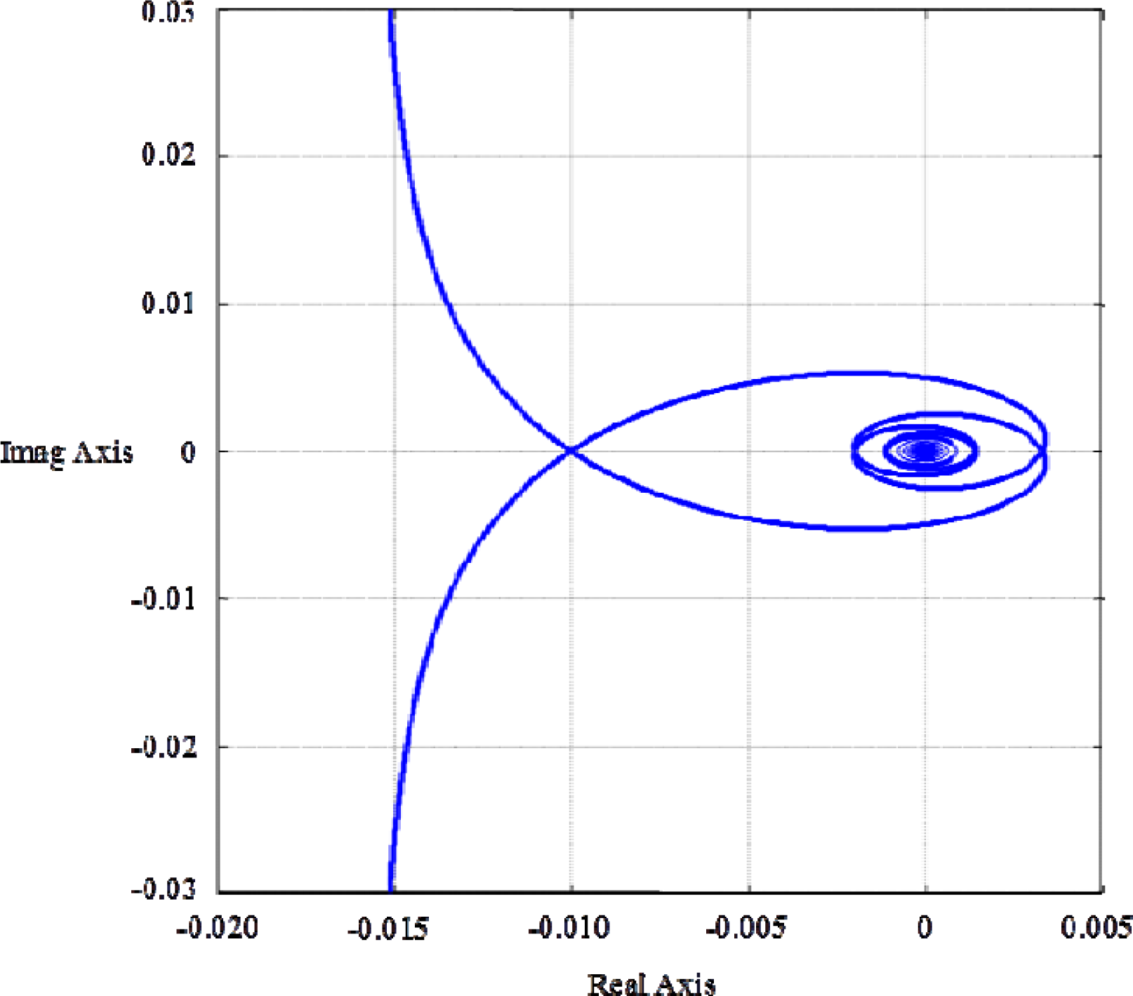
Figure 2 shows the Nyquist plot e^−τs/s for τ = π/200, which, as can be predicted, has the gain margin 100. This implies that those modes with eigenvalues larger than 100 are all unstable.

Another view on the instability of Equation (32) is provided as follows. The 2D transfer-function in Equation (33) has its poles parameterized by each eigenvalue λ :

$$\frac{e^{-\tau s}}{s}=-\frac{1}{\lambda }\hspace{0.17em}\hspace{0.17em}(\lambda >0)$$

(34)

Since the transfer function e^−τs/s has infinite zeros in the right half-plane (RHP), which can be known from Pades’ approximation of e^−τs by a ratio of polynomials [43], the Root Locus regarding to Equation (34) will go across the imaginary axis into the RHP as the positive gain λ is large enough. Therefore, there are always poles of the 2D transfer function in Equation (33) being in the RHP. That is, the perturbation dynamics in Equation (32) is unstable, as proved in the preceding paragraph.

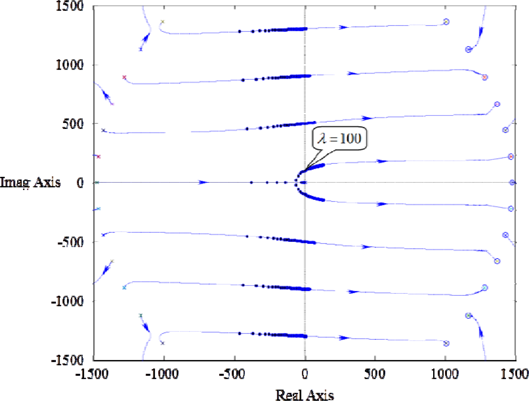
Figure 3 is the Root Locus of 1 + λe^−τs/s = 0 (λ ≥ 0) for τ = π/200. It shows that the transfer function in Equation (33) starts to have RHP poles when the eigenvalue λ is larger than 100, and are getting more RHP poles along with the increase of λ. This yields the same message as that from the Figure 2, in which the Nyquist plot of the transfer-function in Equation (33) begin to encircle (−1,0) as the eigenvalue λ is larger than 100, and the number of encirclements is increased with larger λ.

As of such, even the time-delay in heat diffusion is infinitesimally small, no steady-states of temperature will be possibly observed. The inexistence of observably steady states arises from the ill-posedness of the mathematical modeling, instead of the size of parameter- the time delay in heat diffusion. This implies that the realization of non-Fourier phenomena by the time-delay in heat diffusion is contrary to the truth. Specifically, consider the heat-transfer domain Ω is insulated from heat source across the boundary, i.e., on the boundary of which gradients of temperature are zero. With the same analysis, this heat-transfer dynamics can be proved to be internally unstable. That is, even a tiny heat-flux pulse input to the domain triggers the temperature distributions to be unbounded. This implies that thermal potential (or the internal energy) is infinite due to a finite energy input to the domain, which obviously contradicts the first law of thermodynamics.

4. Thermal Inertia Parameterization

Once thermal inertia does not come from time-delayed diffusion of heat, let us consider the electro-thermal analogy in this section.

The Fourier heat-conduction is a coupling of the heat diffusion:

$$-k\nabla T=\mathit{q}$$

(35)

and the energy conservation:

$$\rho C_v\dot{T}=-\nabla \cdot \mathit{q}+\mathit{Q}$$

(36)

where k stands for the thermal conductivity, ρ for the mass density, C_v for specific heat (at constant volume), and Q for the heat generation. On grounds of electro-thermal analogy, where we choose the temperature T as a thermal voltage and the heat-flux q as a thermal current, it is inferred from Equations (35) and (36) that a differential element is of the thermal resistance being R = 1/k and the thermal capacitance being C = ρC_v.

To fulfill the electro-thermal analogy, we include thermal inductance L into Equation (35) to capture the thermal inertial observed in Non-Fourier heat transfer:

$$-\nabla T=R\mathit{q}+L\dot{\mathit{q}}$$

(37)

and write Equation (36) as:

$$C\dot{T}=-\nabla \cdot \mathit{q}+Q$$

(38)

Equations (37) and (38) represent the heat-conduction in a differential element as an infinitesimal RLC circuit. Application of Kirchhoff’s theorems or careful combination of Equations (37) and (38) yields a hyperbolic equation:

$$L\frac{{\partial }^{2}T}{\partial t^2}+R\frac{\partial T}{\partial t}-\frac{1}{C}{\nabla }^{2}T=\frac{L}{C}\frac{\partial Q}{\partial t}+\frac{R}{C}Q$$

(39)

The equilibrium point T̄ is the same as that of the parabolic equation governing Fourier heat-conduction, and the perturbation ψ imposed on T̄ is governed by:

$$\frac{{\partial }^2\psi }{\partial t^2}+\frac{R}{L}\frac{\partial \psi }{\partial t}-\frac{1}{LC}{\nabla }^2\psi =\frac{1}{C}\frac{\partial Q^{\prime }}{\partial t}+\frac{R}{LC}{Q}^{\prime }$$

(40)

with a homogeneous boundary condition:

$$\nabla \psi =0\hspace{0.17em}\hspace{0.17em}\hspace{0.17em}\hspace{0.17em}\text{or}\hspace{0.17em}\hspace{0.17em}\hspace{0.17em}\hspace{0.17em}\hspace{0.17em}\hspace{0.17em}\psi =0\hspace{0.17em}\hspace{0.17em}\hspace{0.17em}\hspace{0.17em}\hspace{0.17em}\text{on}\hspace{0.17em}\hspace{0.17em}\hspace{0.17em}\hspace{0.17em}\hspace{0.17em}\hspace{0.17em}\partial \Omega$$

(41)

Let us choose a characteristic length ℓ indicating the size of the heat-conduction domain Ω and a characteristic time τ indicating the time lag in heat diffusion τ ≡ L/R, together with a referenced temperature T_r, to make independent and dependent variables in Equations (41) and (42) dimensionless through:

$$x\to x/\ell ;\hspace{0.17em}\hspace{0.17em}\hspace{0.17em}\hspace{0.17em}\hspace{0.17em}t\to t/\tau ;\hspace{0.17em}\hspace{0.17em}\hspace{0.17em}\hspace{0.17em}\hspace{0.17em}\hspace{0.17em}\psi \to \psi /T_r$$

(42)

Substituting those dimensionless variables in Equation (42) into Equations (40) and (41) yields a non-dimensional equation:

$$\frac{{\partial }^2\psi }{\partial t^2}+\frac{\partial \psi }{\partial t}-\kappa {\nabla }^2\psi =\frac{\partial u}{\partial t}+u,\hspace{0.17em}\hspace{0.17em}\hspace{0.17em}\left(\kappa =\frac{{\tau }^2}{{\ell }^2}\frac{1}{LC}\right)$$

(43)

$$\nabla \psi =0\hspace{0.17em}\hspace{0.17em}\hspace{0.17em}\hspace{0.17em}\hspace{0.17em}\text{or}\hspace{0.17em}\hspace{0.17em}\hspace{0.17em}\hspace{0.17em}\hspace{0.17em}\psi =0\hspace{0.17em}\hspace{0.17em}\hspace{0.17em}\hspace{0.17em}\hspace{0.17em}\hspace{0.17em}\hspace{0.17em}\text{on}\hspace{0.17em}\hspace{0.17em}\partial {\Omega }_0$$

(44)

where Ω₀ stands for the normalized domain of heat conduction, u ≡ τQ′/CT_r for the dimensionless entropy flow-rate into the heat-transfer domain, and κ ≡ τ²/ℓ² ·(LC⁻¹) for the amplification factor of eigenvalues of the negative Laplacian −∇² defined on the normalized domain Ω₀.

Performing Laplace-Galerkin transform $\mathscr{H}$ on both sides of Equation (43) yields the 2D transfer-function G of the hyperbolic heat-conduction dynamics of Equations (43) and (44) to be:

$$G(s,\lambda )=\frac{s+1}{s^2+s+\lambda }$$

(45)

Since λ ≥ 0 for all λ ∈ Λ, all poles of G(s) are in the left-half plane (LHP), or possibly, there is a single pole at the origin and the others are in LHP. This implies that the perturbation dynamics in Equation (40) around the unique equilibrium T̄ is always internally stable, and therefore the hyperopic formulation of Non-Fourier heat transfer is of passivity and well-posedness. Given the heat generation u and the initial conditions: ψ₀(x) ≡ ψ(x, 0); ψ_0,t(x) ≡ ∂ψ/∂t(x, 0), one can perform the Laplace-Galerkin transform to yield:

$$\Psi (\lambda ,s)=\frac{(s+1)\cdot U(\lambda ,s)+s\cdot \mathbf{𝒢}{\psi }_0+\mathbf{𝒢}({\psi }_0+{\psi }_{0,t})}{s^2+s+\lambda }$$

(46)

Then he/she can perform the inverse Laplace-Galerkin transform $\mathscr{H}$^-1 to obtain the temperature transience ψ(x, t):

$$\psi (x,t)=\sum _{\lambda \in \Lambda }{\mathbf{ℒ}}^{-1}[\Psi (\lambda ,s)]$$

(47)

The transfer function of Equation (45) reveals that the λ -mode response possesses a damping ratio $\xi \equiv 1/2\sqrt{\lambda }$ and natural frequency $\omega =\sqrt{\lambda }$, where the ratio of every λ ∈ Λ to its corresponding eigenvalue of −∇² on the normalized domain Ω₀ is κ ≡ τ²/ℓ² · (LC⁻¹). As this dimensionless quantity κ is getting larger, thermal inertia is getting easy to be observed. We give it a name: 2nd-sound number.

5. Measurement Instrumentation Design

The parameterization of thermal inertia into thermal inductance makes possible to design a measurement instrument to perform parametric identification.

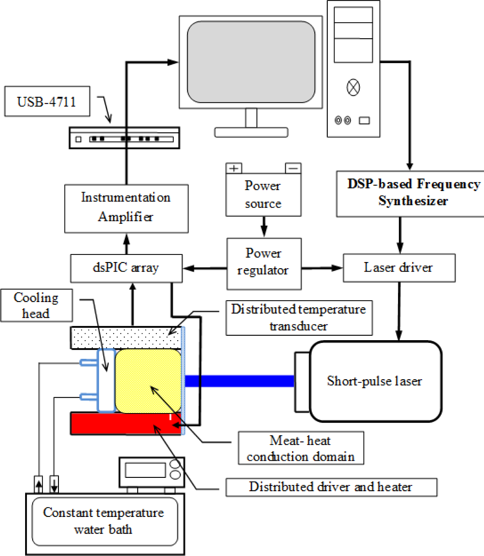
As shown in Figure 4, the instrument to measure thermal inductance comprises a short-pulse laser and its driver for boundary actuation, low-frequency limit-cycle generator, USB4711 data acquisition, Matlab-to-dsPIC networking, distributed temperature sensor and cooler/heater, instrumentation amplifiers, constant-temperature heat sinker, and some supported mechanism. Meat is firstly chosen as the heat-conduction material. The short-pulse laser inputs pulse-width modulated (PWM) thermal current to the right boundary of the conduction material, where the temperature is converted by K-type thermocouples into voltage signals that are tremendously amplified by the instrumentation amplifier and then acquisitioned into a generous-purpose computer through USB4711 communication. The Matlab-to-PIC software is made for integration of dynamics synthesis in the generous-purpose computer and implementation of dynamics into DSP-based controllers. The DSP-based limit-cycle generator plays as the frequency synthesizer of the PWM duty of heat flow from the short-pulse laser.

We collect as the frequency response y of the heat conduction the steady-state sinusoidal responses across a span of input frequencies of heat flow u imposed on a preset DC-level. Temporal responses can further be sent into spectrum-decomposition to calculate out reliable amplitude ratios, figuring out a Bode magnitude plot. Based on Equation (45), the dimensionless frequency response in this experimental setup is

$$G(j\omega )\equiv \frac{Y(j\omega )}{U(j\omega )}=\sum _{\lambda \in \Lambda }\frac{j\omega +1}{{(j\omega )}^2+j\omega +1}{\varphi }^2(\lambda ,0)$$

(48)

where the modulus |G(jω)| and argument ∠G(jω) indicates the amplitude ratio and phase difference, respectively, of the output to the input as the input frequency is ω. Figure 5 shows the Bode magnitude plot according to Equation (48), wherein Fourier heat-conduction is also plotted in dotted lines for comparison.

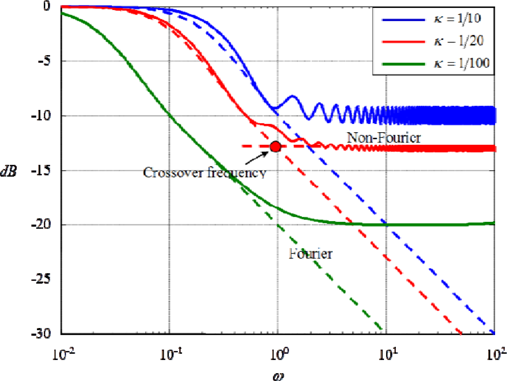
The Bode plot in Figure 5 shows special frequency responses in a non-dimensional fashion, dubbed thermal hyperbolicity, listed as follows:

(1)

As opposed to the parabolic Fourier heat-conduction, the amplitude ratio of which is monotonically decreasing with the input frequency, the amplitude ratio of Non-Fourier heat-conduction is no longer decreasing in average after crossing some certain frequency named crossover frequency.

(2)

After the crossover frequency, the amplitude ratio exhibits a series of resonant ripples at natural frequencies of all modes. The amplitudes of ripples are getting larger along with the increasing 2nd-sound number κ.

(3)

Before the crossover frequency, the decay rate of amplitude ratio is reduced along with increase of the 2nd-sound number κ. Any Non-Fourier heat-conduction has smaller decay rate than that of Fourier heat-conduction, which is nearly 10 dB per log ω.

(4)

Since larger amplitude ratios follows larger 2nd-sound number κ, identification of thermal inductance in frequency domain is more accurate in a smaller scaled heat-conduction domain.

With these special properties, we are able to accurately and reliably identify thermal inductance in the frequency domain by adjusting the length of heat-conducting materials. Note that the thermal vibration implied in the non-dimensional modeling of Equation (43) involves a constant damping across all modes. This means that the damping ratio of each mode is inversely proportional to the square-root of its stiffness. In the Bode plot, both higher stiffness and damping ratio yield smaller amplitude ratios and both effects arrive at a balance after the crossover frequency.

To fulfill frequency-domain identification, a limit-cycle generator is programmed into a microcontroller embedded with a DSP engine (named by DSP-controller), frequencies of which are adjustable in a real-time fashion. In this work, we generalize the van der Po oscillator as the nominated limit-cycle generator. The van der Pol oscillator is a non-conservative oscillator with non-linear damping, which evolves in time according to the second order differential equation. Let us consider a more general class of van der Pol oscillators as:

$$\ddot{y}+\mu (y^2-\frac{a^2}{4})\dot{y}+{\omega }^{2}y=0;\hspace{0.17em}\hspace{0.17em}\hspace{0.17em}\hspace{0.17em}\hspace{0.17em}\hspace{0.17em}\mu >0$$

(49)

where y is the output, and three parameters- a, ω and μ are to be adjusted. The dynamics of Equation (49) generates a sustained oscillation with amplitude a and angular frequency ω in steady state, and the transience period is getting shorter along with increasing value of μ.

In our design, the frequency synthesizer is fulfilled by series of such a van der Pol oscillator with a first-order low-pass filter to shape outputs into a pure sinusoidal function even when μ is large at will for ultra short transience. Accordingly, the frequency synthesizer is the van der Pol dynamics:

$$\begin{array}{l}\ddot{z}+{\omega }^{2}z=u\\ u=-\mu \left(z^2-\frac{a^2}{4}\right)\dot{z}\end{array}$$

(50)

which has been represented by internal feedback-interconnection, in series with the first-order filter:

$$\tau \dot{y}+y=\sqrt{2}z\hspace{0.17em}\hspace{0.17em}\hspace{0.17em}\hspace{0.17em}(\tau =1/\omega )$$

(51)

By choosing three state variables: x₁ = z, x₂= ż, and x₃ = y, the state-space realization of this limit-cycle generator becomes:

$$u=-\mu \left(x_1^2-\frac{a^2}{4}\right)x_2$$

(52)

$$\left[\begin{array}{c}{\dot{x}}_1\\ {\dot{x}}_2\\ {\dot{x}}_3\end{array}\right]=\left[\begin{array}{ccc}0& 1& 0\\ -{\omega }^2& 0& 0\\ \sqrt{2}\omega & 0& -\omega \end{array}\right]\left[\begin{array}{c}{x}_1\\ x_2\\ x_3\end{array}\right]+\left[\begin{array}{c}0\\ 1\\ 0\end{array}\right]u$$

(53)

$$y=\left[\begin{array}{ccc}0& 0& 1\end{array}\right]\left[\begin{array}{c}{x}_1\\ x_2\\ x_3\end{array}\right]$$

(54)

It appears as a feedback-interconnected LPV form: u = f(x; μ, a); ẋ = A(ω)x + Bu; y = Cx, where the command (angular) frequency ω, amplitude a and converging speed μ constitute the slow-time parameter that will be on-line scheduled in a slow-time fashion.

The frequency synthesizer in Equation (53) is then implemented into a DSP-engine embedded microcontroller with the Linear Parameter-varying Matrix Iteration Time-fixed (LPV-MIT) method as follows. Continuous-to-digital conversion of Equation (53) arrives at:

$$\begin{array}{l}{u}_k=f(x_k;{\mu }_j,a_j)\\ x_{k+1}=\Phi ({\omega }_j)x_k+\Gamma ({\omega }_j)u_k\\ y_k=C{x}_k\end{array}$$

(55)

where k and j are fast-time and slow-time indexes, respectively, and the system matrices (Φ, Γ) will be calculated on-line in a slow-time fashion since the resonant frequency ω is slow-time updated in practice. Explicitly:

$$\Phi ({\omega }_j)=e^{A({\omega }_j)}\approx \sum _{i=0}^n\frac{A^i({\omega }_j)T^i}{i!}$$

(56)

$$\Gamma ({\omega }_j)\approx T\sum _{i=1}^n\frac{A^{i-1}({\omega }_j)T^{i-1}}{i!}$$

(57)

where T is the fast-time sampling period that is short enough to make the above Taylor-series expansion accurate even with few terms, say, n = 2 or 3 as T is 0.001 second.

At the present time t_k the DSP-controller merely stores the current state x_k, and the update of state from x_k to x_k+1 at next instant is fulfilled by DSP engine performing the addition and multiplication of floating numbers according to Equation (54). In that sense, any time can be treated as the initial time, which makes real-time processing most efficient. Moreover, the state update intervals are held identical to those in computer simulation, so that the real-timed operation matches the dynamics that has been verified by offline calculation, thus achieving robust implementation. At any instance, a pulse-width modular (PWM) signal in line with the output y is sent to the gate-driving circuit of switched power converters that drive the short-pulse laser.

6. Thermal Inductance Identification

With the instrument and instrumentation designed above, we start to measure temperature responses of meat excited by the short-pulse laser.

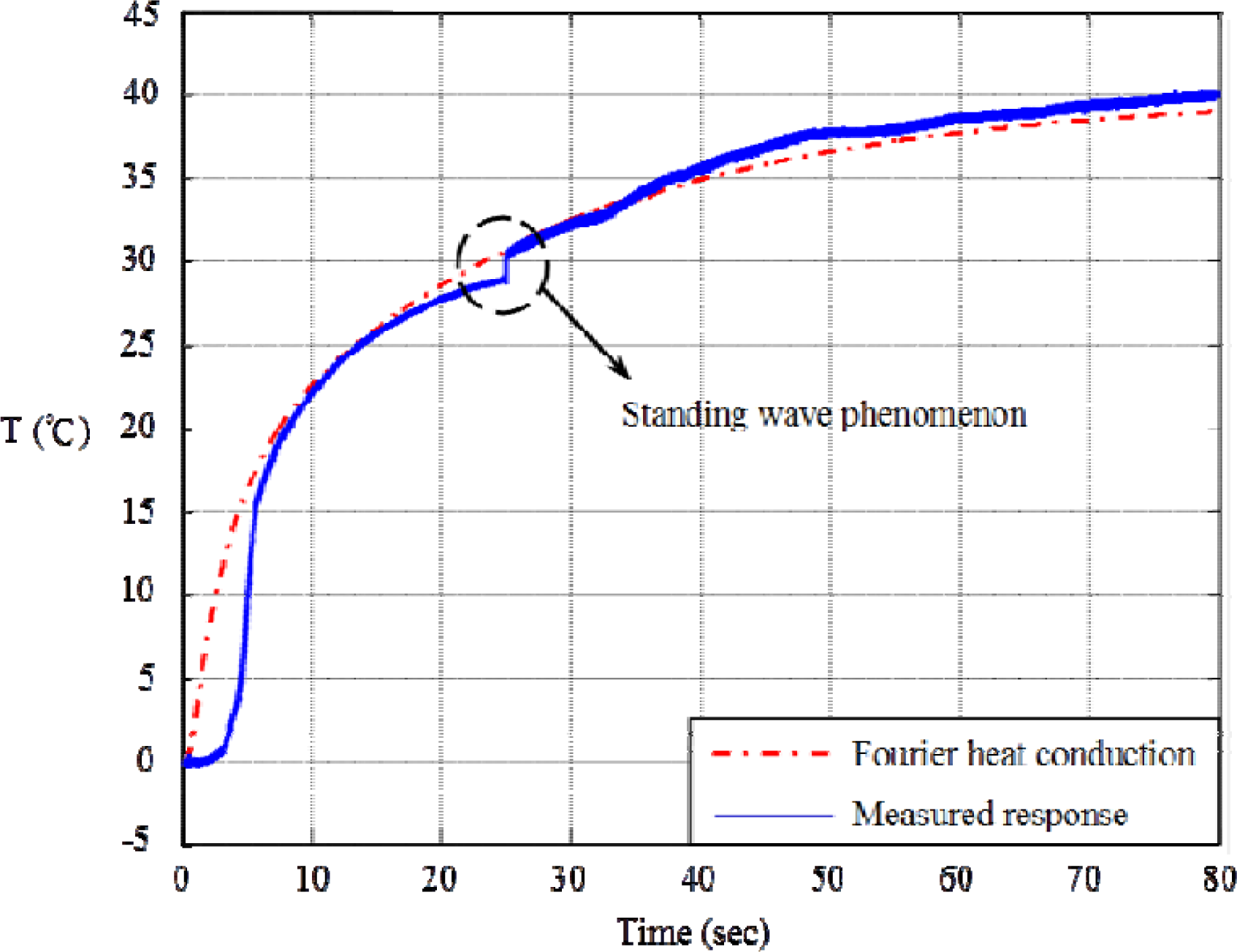
Figure 6 shows the typical responses as the laser delivers a series of pulses to the right boundary. Compared with the calculated response of Fourier heat-conduction, the measured non-Fourier response exhibits diffusion lagging initially, but quickly they are indistinguishable to each other until the thermal wave is reflected from the left end back to the right end as a small jump to be measured. This standing wave behavior is getting obvious as the length of meat is cut shorter. However, we find that the identification of thermal inductance through the measurement of standing-wave behavior is unreliable. Similar problems also happen at other measurements in time domain, wherein catching the jump with high-bandwidth sensing is always severely contaminated by white-noise, and filtering out white-noise often seriously degrades the jump-signal.

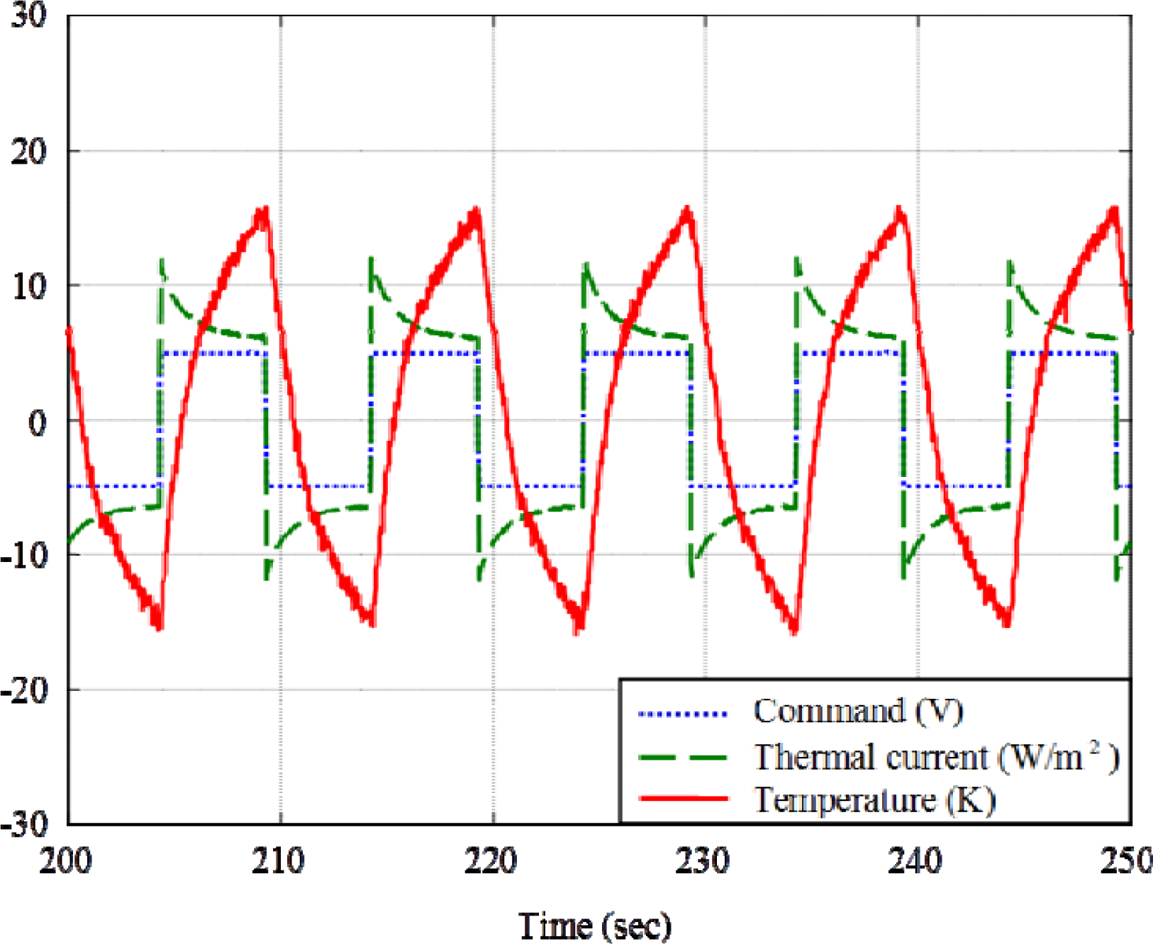
Figure 7 shows the step response as the control signal to laser is a series of steps. Although the time constant therein reveals the information of thermal inductance, however, it is very close to that of Fourier heat-conduction. Moreover, as observed, the corresponding thermal current into the heat-conduction domain is not a pure step, so identification of thermal inductance with step responses is inaccurate or unreliable. Identification of thermal inductance in frequency domain is the most reliable because:

(1)

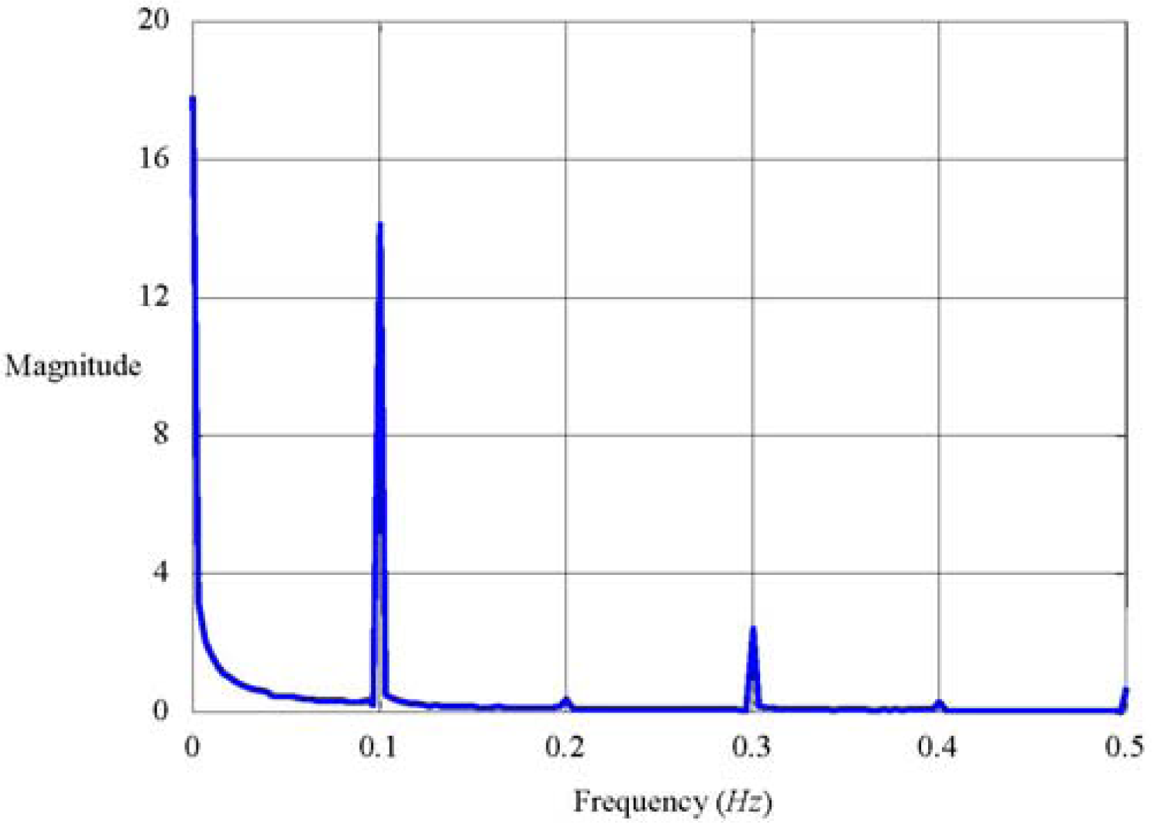
The noisy contamination of amplitude ratio can be perfectly removed with spectrum decomposition since merely the component at the input frequency is concerned, as shown in Figure 8.

(2)

The crossover frequency quantifies the thermal inductance and it is against any uncertainties that can happen, such as the real values of amplitude ratios.

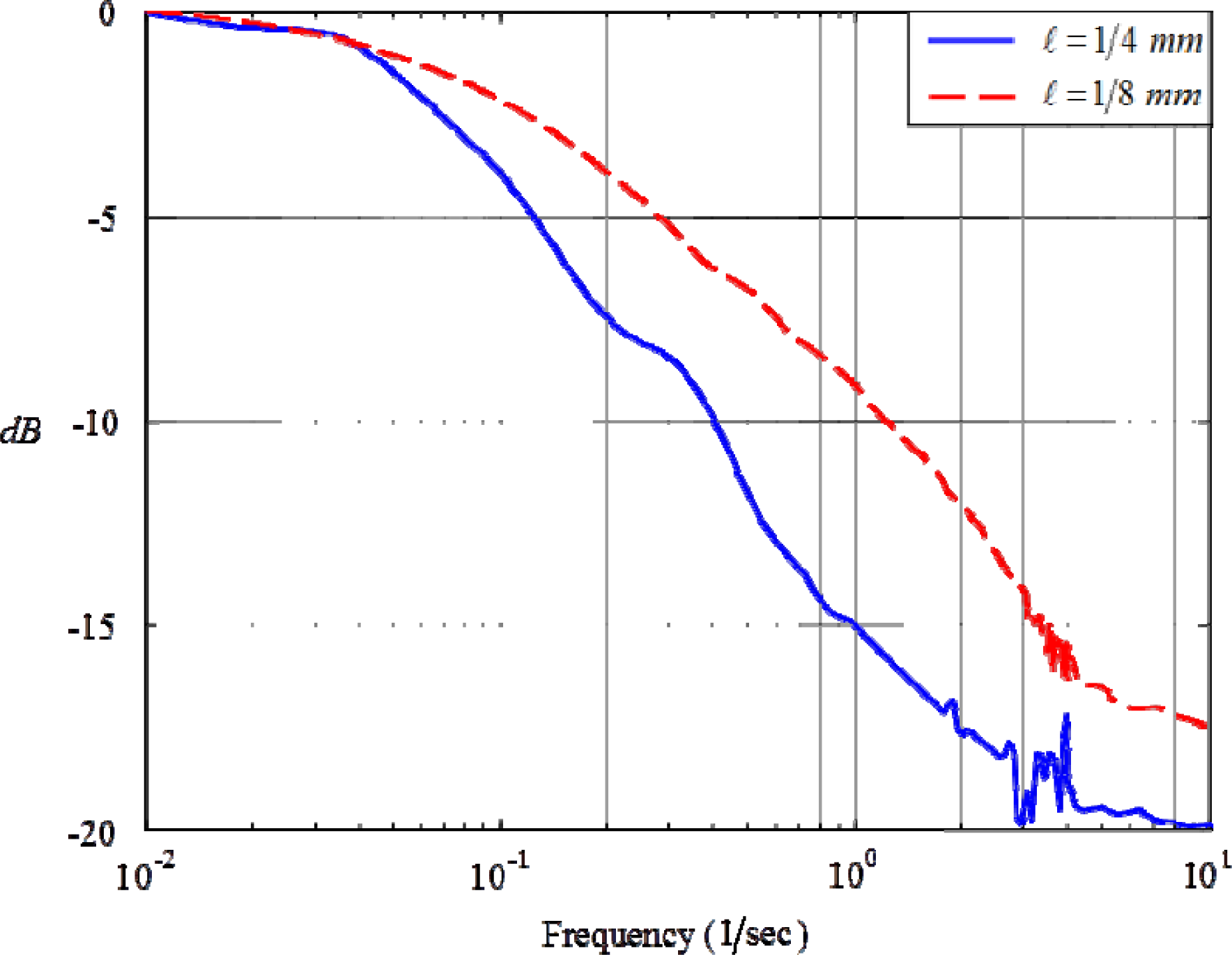
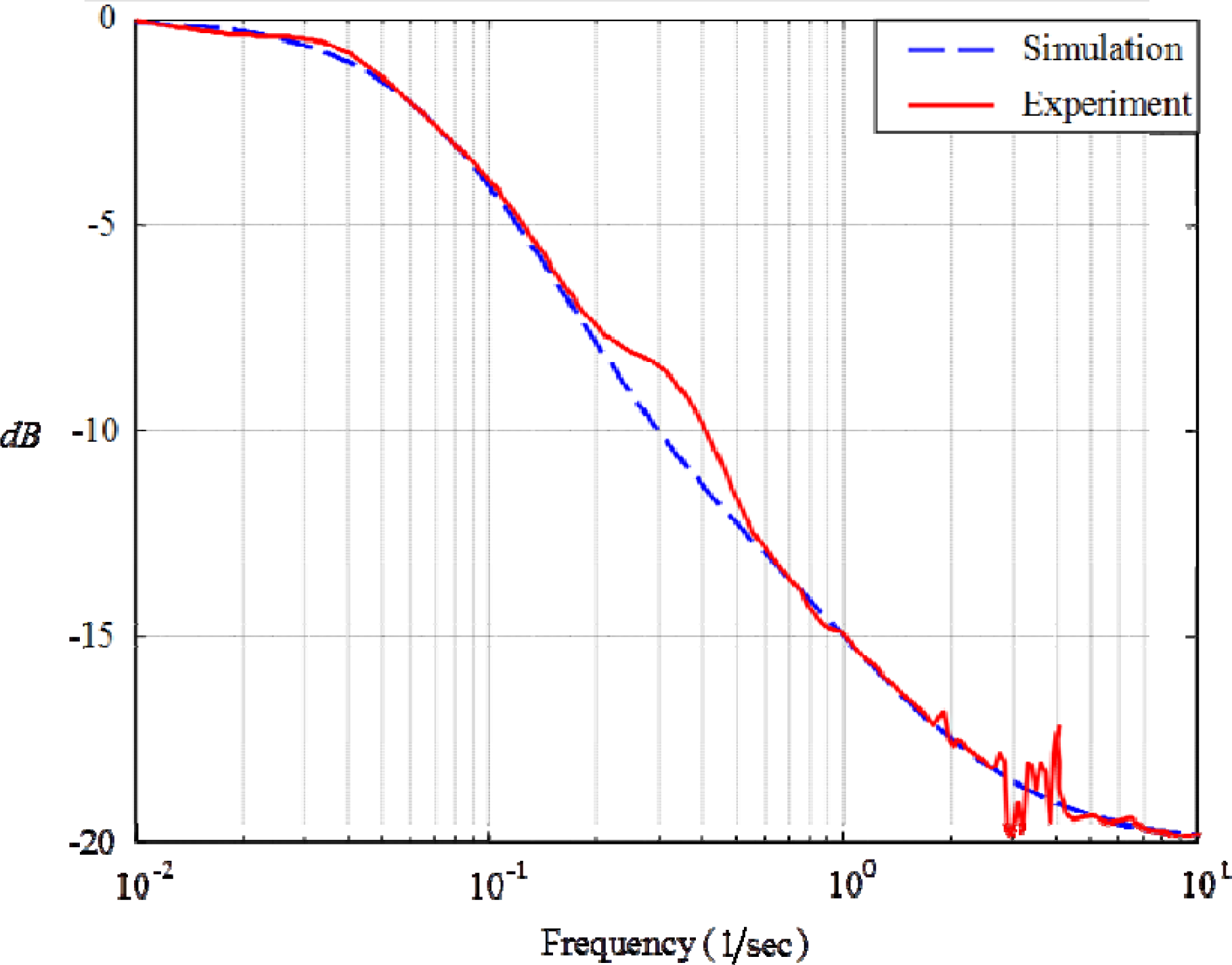
Figure 9 records the measured Bode plot upon 0.25 mm-length meat, wherein there are 130 points ranged from 0.01 Hz to 10 Hz. This Bode plot evidently reveals the thermal hyperbolicity resulted from parameterization of thermal inertia into thermal inductance, and the crossover frequency being 4 Hz. This verifies the electro-thermal analogy and identify the thermal inductance with L = 3.83 s · m· K/W. In advance, we have measure the following quantities for the processed meat at 25 °C: the density ρ = 980 kg/m³, the specific heat-ratio C_v = 3900 J/kg · K, and the heat-conduction coefficient k = 0.71 W/m · K. Figure 10 records the Bode plot as the length of meat is further cut shorter to be 0.125 mm. Since the 2nd-sound number has doubled, the frequency response exhibits larger level of thermal hyperbolicity, making measurement of thermal inductance less noise-contaminated. Suppose the experimental rig had supported micro-scaled heat-transfer domain, the thermal inertia would have clearer view in the Bode plot. With this kind of instrumentation, we measure thermal inductances at a variety of environmental temperatures.

Table 1. Thermal parameters measured at 25 degrees centigrade.

Material	Thermal Resistance (m·K/W)	Thermal Capacitance (J/m3·k)	Thermal Inductance (s·m·K/W)
Agar	1.646	4,170,451	6.01
Processed meat	1.179	4,069,800	3.83
Sand	0.8	1,488,960	1.24
NaHCO3	1.42	2,246,400	2.37

lists the other three materials at room temperature.

The finding of thermal inductance gives us fresh impetus to manufacture storages of thermal kinetics, and to control the thermal vibrations in small-scaled or fast-timed scaled heat-transfer dynamics.

7. Conclusions

We have mathematically proved that the time-delayed parabolic equation is ill-posed. This implies that the realization of thermal inertia by the time-delay violates the law of energy conservation. Continuing from this theoretical work, we further verify experimentally that the thermal inertia can be parameterized by the thermal inductance, which becomes a new physical quantity. Thanks to the found thermal hyperbolicity in the frequency domain, instrumentation can be designed for robust identification of thermal inductances, wherein a novel DSP-based frequency synthesizer is developed specially for frequency-domain identification. The existence of thermal inductance implies a new possibility for energy storage in analogy to inductive energy storage in electricity or mechanics.

References

- Bosworth, B.C.L. Thermal inductance. Nature 1946, 158, 309. [Google Scholar]
- Bosworth, B.C.L. Thermal mutual inductance. Nature 1948, 161, 166–167. [Google Scholar]
- Kaminiski, W. Hyperbolic heat conduction equation for materials with a non-homogeneous inner structure. J. Heat Transf.-Trans. ASME 1990, 112, 555–560. [Google Scholar]
- Vedavarz, A.; Mitra, K.; Kumar, S.; Moallemi, M.K. Effect of Hyperbolic Conduction on Temperature Distribution in Laser Irradiated Tissue with Blood Perfusion. In Advances in Biological Heat and Mass Transfer; McGrath, J.J., Ed.; ASME: New York, NY, USA, 1992; pp. 7–16. [Google Scholar]
- Vedavarz, A.; Kumar, S.; Moallemi, M.K. Significance of non-Fourier heat waves in conduction. J. Heat Transf.-Trans. ASME 1994, 116, 221–224. [Google Scholar]
- Roetzel, W.; Putra, N.; Das, S.K. Experiment and analysis for non-Fourier conduction in materials with non-homogeneous inner structure. Int. J. Therm. Sci 2003, 42, 541–552. [Google Scholar]
- Mitra, K.; Kumar, S.; Vedavarz, A.; Moallemi, M.K. Experimental evidence of hyperbolic heat conduction in processed meat. J. Heat Transf.-Trans. ASME 1995, 117, 568–573. [Google Scholar]
- Jiang, F.; Liu, D.; Zhou, J. Non-Fourier heat conduction phenomena in porous material heated by microsecond laser pulse. Nanoscale Microscale Thermophys. Eng 2002, 6, 331–346. [Google Scholar]
- Sousa, R.A.D.; Rocha, A.F.D.; Schutt, D.; Haemmerich, D.; Santos, E.I.D. Experimental Evidence of Hyperbolic Heat Conduction in Agar. In Proceedings of the 21th Congresso Brasileiro de Engenharia Biomédica (CBEB), Salvador-Bahia, Brazil, 16–20 November 2008; pp. 1343–1346.
- Liu, C.; Mi, C.-C.; Li, B.-Q. Transient temperature response of pulsed-laser-induced heating for nanoshell-based hyperthermia treatment. IEEE Trans. Nanotechnol 2009, 8, 697–706. [Google Scholar]
- Fan, J.; Wang, L. Analytical theory of bioheat transport. J. Appl. Phys 2011, 109, 10472. [Google Scholar]
- Tzou, D.-Y. Lagging behavior in biological systems. J. Heat Transf.-Trans. ASME 2012, 134. [Google Scholar] [CrossRef]
- Maxwell, J.C. On the dynamic theory of gases. Philos. Trans. R. Soc. Lond 1867, 157, 49–88. [Google Scholar]
- Nernst, W. Die Theoretischen und Experimentellen Grundlagen des Neuen Warmesatzes; Knapp: Halle, Germany, 1918. (In German) [Google Scholar]
- Peshkov, V. Second sound in helium II. J. Phys. USSR 1944, 8, 381. [Google Scholar]
- Taitel, Y. On the parabolic, hyperbolic and discrete formulation of the heat conduction equation. Int. J. Heat Mass Transf 1972, 15, 369–371. [Google Scholar]
- Joseph, D.D.; Preziosi, L. Heat waves. Rev. Mod. Phys 1989, 61, 41–73. [Google Scholar]
- Mandrusiak, G.D. Analysis of non-Fourier conduction waves from a reciprocating heat source. J. Thermophys. Heat Transf 1997, 11, 82–89. [Google Scholar]
- Tan, Z.M.; Yang, W.J. Heat transfer during asymmetrical collision of thermal waves in a thin film. Int. J. Heat Mass Transf 1997, 40, 3999–4006. [Google Scholar]
- Honner, M. Heat waves simulation. Comput. Math. Appl 1999, 38, 233–243. [Google Scholar]
- Al-Nimr, M.A.; Alkam, M.K. Overshooting phenomenon in the hyperbolic microscopic heat conduction model. Int. J. Thermophys 2003, 24, 577–583. [Google Scholar]
- Hermann, R.P.; Grandjean, F.; Long, G.J. Einstein oscillators that impede thermal transport. Am. J. Phys 2005, 73, 110–118. [Google Scholar]
- Cattaneo, C. Sulla conduzione del calore. Atti Del Seminar. Mat. Fis. Univ. Modena 1948, 3, 83–101. (In Italian). [Google Scholar]
- Cattaneo, C. A form of heat conduction equation which eliminates the paradox of instantaneous propagation. Compte Rendus 1958, 247, 431–433. [Google Scholar]
- Vernotte, P. Les paradoxes de la theorie continue de l’equation de la chaleur. Comput. Rendus 1958, 246, 3154–3155. (In French). [Google Scholar]
- Vernotte, P. Some possible complications in the phenomena of thermal conduction. Compte Rendus 1961, 252, 2190–2191. [Google Scholar]
- Hong, B.-S. Construction of 2D isomorphism for 2D H∞-control of Sturm-Liouville systems. Asian J. Control 2011, 12, 187–199. [Google Scholar]
- Tzou, D.Y. Macro- to Microscale Heat Transfer: The Lagging Behavior; Taylor & Francis: Washington, DC, USA, 1997. [Google Scholar]
- Ichiyanagi, M. Comments on the entropy differential in extended irreversible thermodynamics. Kyoto Univ. Res. Inf. Repos 1997, 982, 220–233. [Google Scholar]
- Hong, B.-S.; Su, P.-J.; Chou, C.-Y.; Hung, C.-I. Realization of non-Fourier phenomena in heat transfer with 2D transfer function. Appl. Math. Model 2011, 35, 4031–4043. [Google Scholar]
- Basirat Tabrizi, H.; Andarwa, S. A method to measure time lag constants of heat conduction equations. Int. Commun. Heat Mass Transf 2009, 36, 186–191. [Google Scholar]
- Tassart, S. Band-limited impulse train generation using sampled infinite impulse responses of analog filters. IEEE Audio Speech Lang. Process 2013, 21, 488–497. [Google Scholar]
- Wang, G.; Yang, R.; Xu, D. DSP-based control of sensorless IPMSM drives for wide-speed range operation. IEEE Trans. Ind. Electron 2013, 60, 720–727. [Google Scholar]
- Hong, B.-S.; Lin, T.-Y.; Su, W.-J. Electric Bikes Energy Management-Game-Theoretic Synthesis and Implementation. In Proceedings of the 2009 IEEE International Symposium on Industrial Electronics (ISIE), Seoul, Korea, 5–8 July 2009; pp. 2131–2136.
- Yeary, M.B.; Fink, R.J.; Beck, D.; Guidry, D.W.; Burns, M. A. DSP-based mixed-signal waveform generator. IEEE Trans. Instrum. Meas 2004, 53, 663–671. [Google Scholar]
- Madheswaran, M.; Menakadevi, T. An improved direct digital synthesizer using hybrid wave pipelining and CORDIC algorithm for software defined radio. Circuits Syst. Signal Process 2003, 32, 1219–1238. [Google Scholar]
- De Caro, D.; Napoli, E.; Strollo, A.G.M. Direct digital frequency synthesizers with polynomial hyperfolding technique. IEEE Trans. Circ. Syst. II Exp. Briefs 2004, 51, 337–344. [Google Scholar]
- O’Leary, P.; Maloberti, F. A direct-digital synthesizer with improved spectral performance. IEEE Trans. Commun 1991, 39, 1046–1048. [Google Scholar]
- Vankka, J.; Waltari, M.; Kosunen, M.; Halonen, K.A.I. A direct digital synthesizer with an on-chip D/A-converter. IEEE J. Solid-St. Circ. 1998, 33, 218–227. [Google Scholar]
- Yang, B.-D.; Choi, J.-H.; Han, S.-H.; Kim, L.-S.; Yu, H.-K. An 800-MHz low-power direct digital frequency synthesizer with an on-chip D/A converter. IEEE J. Solid-St. Circ 2004, 39, 761–774. [Google Scholar]
- Yeoh, H.C.; Jung, J.-H.; Jung, Y.-H.; Baek, K.-H. A 1.3-GHz 350-mW hybrid direct digital frequency synthesizer in 90-nm CMOS. IEEE J. Solid-St. Circ. 2010, 45, 1845–1855. [Google Scholar]
- Young, N. An Introduction to Hilbert Space; Cambridge University Press: New York, NY, USA, 1992. [Google Scholar]
- Franklin, G.F.; Powell, J.D.; Emami-Naeini, A. Feedback Control of Dynamic Systems; Addison-Wesley: Boston, MA, USA, 1994. [Google Scholar]