Fast Feature Selection in a GPU Cluster Using the Delta Test

 ,
,
Abstract
: Feature or variable selection still remains an unsolved problem, due to the infeasible evaluation of all the solution space. Several algorithms based on heuristics have been proposed so far with successful results. However, these algorithms were not designed for considering very large datasets, making their execution impossible, due to the memory and time limitations. This paper presents an implementation of a genetic algorithm that has been parallelized using the classical island approach, but also considering graphic processing units to speed up the computation of the fitness function. Special attention has been paid to the population evaluation, as well as to the migration operator in the parallel genetic algorithm (GA), which is not usually considered too significant; although, as the experiments will show, it is crucial in order to obtain robust results.1. Introduction
The problem of variable selection is crucial for the time of the design models that classify or perform regression; so, the better the selection is, the more accurate that models can be designed [1–3]. Although classification and regression are both modeling problems, they should be treated separately. Thus, the work presented in this paper focuses on regression, also known as function approximation. Formally, the function approximation problem is to determine, given a set of input/output pairs (xi,yi) ∈ Rd × R i = 1...N and an unknown function, f, such as f(xi) ≈ yi. From this, the problem of variable selection can be defined as the search for the subset of variables that make it possible to build a model that approximates the data as accurately as possible.
At first, the method to determine the most adequate subset of variables could seem trivial: build a model for each possible solution. This approach could be considered as the brute force approach and would be optimal; however, it has critical problems:
It is not possible to compute all the combinations when the problem has a large number of variables, due to the computational cost;
The validity criterion depends in the model, which usually has several parameters that affect the final results considerably.
These problems have encouraged the use of non-parametric metrics (which are model independent) to be more objective about the time of evaluating a solution. One of the mainstream ways is to use mutual information (MI) [4] as a criterion. MI is defined as the difference between the sum of the individual entropies and the joint entropy and of two events (in the variable selection problem, the events are the output, Y, and the inputs, X). The higher it is, the more relevant for the model the variables selected for X should be. This approach has been successfully applied using several estimators to compute it. Another non-parametric criterion that has been applied to variable selection is the delta test (DT) [5]. There are few papers that apply it, although its adequacy to perform variable selection has been theoretically demonstrated in [6,7]. Concretely, in [7], there are comparisons of DT versus MI using Kraskov’s estimator, where DT shows better performance. A recent comparison between both approaches has been done in [8], where the MI showed a slightly better performance according to experts’ opinions. However, in [9], MI estimation using the Parzen window and Kraskov’s method were outperformed by DT, considering objective metrics as the approximation error using least squares support vector machines and experts’ opinions. The interesting thing about this last paper is that, due to the small number of samples, an exhaustive search is performed, so that the global optimum for each metric is obtained. This encourages the research presented in this paper, because it emphasizes how important it is to analyze as many solutions as possible. Therefore, this work is focused on optimizing a parallel genetic algorithm, which is implemented on a novel high performance computing (HPC) architecture using clusters of computers with several graphical processing units (GPUs). Using this architecture, speed up can be obtained by using GPUs to compute the fitness (in this case, the DT) and CPUs to parallelize the genetic algorithm (GA). Moreover, the parallelization of optimization algorithms seems to be the only way to obtain solutions in large dataset problems, as there are computation and time limitations if a single machine is used. This work presents analyses, as well one of the most important parameters in parallel genetic algorithms: the migration operator.
The rest of the paper is organized as follows: Section 2 introduces the delta test. Afterwards, Section 3 describes the design of the parallel genetic algorithm, which will perform the optimizations presented in the experiments included in Section 4. Finally, conclusions are discussed.
2. Delta Test in Variable Selection
In order to evaluate the goodness of an individual, the delta test (DT) [5] value obtained using the combination of variables is used, as it has been shown to be an adequate criterion [6,10].
In function estimation, the main problem is to find the correct signal and noise terms. As mentioned, the relationship between input (signal) xi and output yi is represented as
The DT is computed using the nearest neighbor approach as:
2.1. Computation of Delta Test Using Pre-Calculated Distances
Computation of the nearest neighbor in the naive way involves calculating the distances between each pair of samples:
2.2. Computation of the Delta Test on a GPU
The computation of the k nearest neighbors (KNN) requires great computational effort, since it has to compute the pairwise distances between all the points and, then, sort them to choose the closest ones. In [12], an implementation of the KNN algorithm on a GPU (the code is available at [13]) is presented. In this approach, brute force is used to compute the distances between the input vectors, as they are independent of each other; therefore, they are easily parallelized using the single instruction multiple data (SIMD) paradigm.
After computing the distances, they need to be sorted to determine the closest neighbors. To do so, the insertion sort algorithm used is Quicksort; due to its recursive nature, it cannot be implemented on GPUs.
All the processes require about 10 times faster speed than other algorithms implemented in libraries, such as ANN (Approximate Nearest Neighbor [14]) which uses kd-trees and box-decomposition trees to improve performance.
Another advantage of using the GPU is that, although the computation is repeated constantly, it allows one to handle large problems, unlike the pre-calculated distance approach, which might have memory limitations.
3. Design of the Genetic Algorithm
Genetic algorithms (GAs) are a well-known optimization tool that has been applied to many problems. This kind of algorithm is based on the principles of natural evolution, where the offspring of the new generations are supposed to be better than their parents. The main advantage of GAs is that they have the ability to explore the solution space globally, but at the same time, they can exploit the regions where the best solutions are.
When a GA is designed, the first decision to be made is how an individual will represent a solution, that is, the solution encoding. The variable selection problem has a straightforward encoding using a binary chromosome, whose length is equal to the number of variables. If a gene within the chromosome equals one, the variable is selected; if it is zero, then the variable is discarded.
Once the encoding of the solutions is defined, it is necessary to determine the operators that will affect the evolution of the individuals. These are introduced in the following subsections.
3.1. GA Operator Description
There are several types of operators that will modify the chromosome of an individual. The first one is the selection operator, which determines if an individual is going to reproduce and generate offspring. If the selection is very restrictive and only the best individuals reproduce, the convergence of the algorithm is accelerated. On the other hand, if random individuals are chosen, there is the risk of not converging to a good solution, as well as a lack of robustness. The chosen operator is “binary tournament selection”, which consists of taking two couples of individuals and selecting from each couple the individual that has better fitness.
The second one is the crossover operator, which is responsible for combining the genes of the parents to produce the offspring. For the binary encoding, many operators have been proposed, although the two-points binary crossover seems to have a compromise between the exploration/exploitation of the solutions [15]. This operator defines two points in the chromosome where the individuals exchange genes, generating two new individuals.
Once the offspring are obtained, they might suffer a mutation in their chromosome. This mutation is the one that helps the algorithm to escape from local minima and jump to other regions of the solution space. The mutation selected was at the gene level, that is, if the individual is mutating, select-unselect a random variable.
Finally, to obtain the population t +1, it has to be decided if the whole population, t, is going to be replaced (generational GA) or only some of the offspring replace their ancestors (stationary GA). As there is the need to obtain a high number of solutions, it is more adequate to use the newly generated individuals, but to maintain exploitation, the best individuals of the previous generation are kept. This is known as elitism [16].
The evolution continues until a stop criterion is satisfied. There are many possibilities and approaches proposed in the literature [17]; however, the proposed algorithm only considers an execution time limit of 600 s. This criterion affects all the previous operators, as well as their parameters (i.e., crossover and mutation probabilities).
The reason for choosing 600 s is because this value is considered as the maximum time an operator is willing to wait before a solution is provided. Even though variable selection is an off − line problem, a human operator might decide to recompute solutions with new collected data at any time. This time limit has been previously used in the literature for GAs [18,19], and it is a common time barrier used in many programs implemented by important companies, like Microsoft [20], Apple [21], Apache [22], etc.
Therefore, the limitation implies that the convergence should be fast, but diversity should still be reasonably maintained. These are the reasons to select the binary tournament (high selection pressure), two-point binary crossover with a high probability of obtaining a high exploitation of the solutions, mutation at a gene level, but with a high probability of maintain exploration, and elitism, to always keep the best chromosomes so far (high exploitation).
To summarize, the standard operators chosen for the algorithm are:
- (1)
Crossover: two-point binary with 0.8 probability.
- (2)
Mutation: gene level with 0.1 probability.
- (3)
Selection: binary tournament selection.
- (4)
Elitism: keep 10% of the best individuals from the previous generation.
- (5)
Stop criterion: 600-s time limit.
3.2. Parallelizing the GA
Apart from the optimization of the computation of the fitness function using GPUs, the available architecture allows the algorithm to be distributed through several machines in a classical cluster manner. GAs are intrinsically parallel in the sense that several operations can be done in parallel, because they are independent. However, modifications in the execution flow, like splitting the populations into sub-populations, also known as demes, lead to better results [23–26].
3.2.1. Island Model and Migration/Immigration Policy
Among the several approaches proposed in the literature to parallelize GAs [27], the multi-deme distributed GA (also known as the island model) is one of the most popular, due to its good behavior [26–28]. This implementation consists of evolving isolated populations on different islands and, in some cases, exchanging individuals. The implementation of this paradigm usually maps an island to a processor. In the available architecture for this work, since a processor might have several cores, populations are mapped to cores. Regarding the use of the GPUs to compute the DT for each individual, an island uses one GPU to compute the distance matrix.
The mechanism that exchanges individuals between the islands is known as the migration operator. The benefits of this procedure can be different, depending on the way it is applied and the criterion that selects the individuals [29]; it can help to maintain diversity by exploring new solutions provided by the new individuals, or it might help exploitation, because all islands will share some equal individuals. The communication between the islands requires one to consider the following parameters:
Send policy: decides which individual or individuals should be sent.
Acceptance policy: decides if one or several individuals coming from other islands are or are not included in the destination island.
Replacement policy: if new individuals are incorporated into the population, this policy must determine which individuals of the current population should be replaced (in order to maintain the population size).
Communication topology: defines the migration flow, that is, between which islands are individuals being exchanging.
Communication frequency: determines when the migration step will be carried out.
The analysis of the GA behavior as a function of the migration process has not been studied deeply since some years ago [30,31], although recent papers study this parameter, as it has an important influence on the results [32,33]. Concretely, in [33], the authors propose the MultiKulti algorithm, whose main novelty is to introduce a criterion that determines if an island accepts a migration or does not. The results presented showed that the diversity and the number of individual evaluations before the algorithm finished increased using this migration filtering.
The migration rate is a parameter that can be random [34], fixed [26] or autoregulated, depending on the diversity of the population. However, to consider the population diversity to modulate the migration rate is equivalent to determining a replacement policy. The reason is that if the replacement policy determination is based as well on the current population and does not accept any replacement, it is as if the migration rate has been decreased.
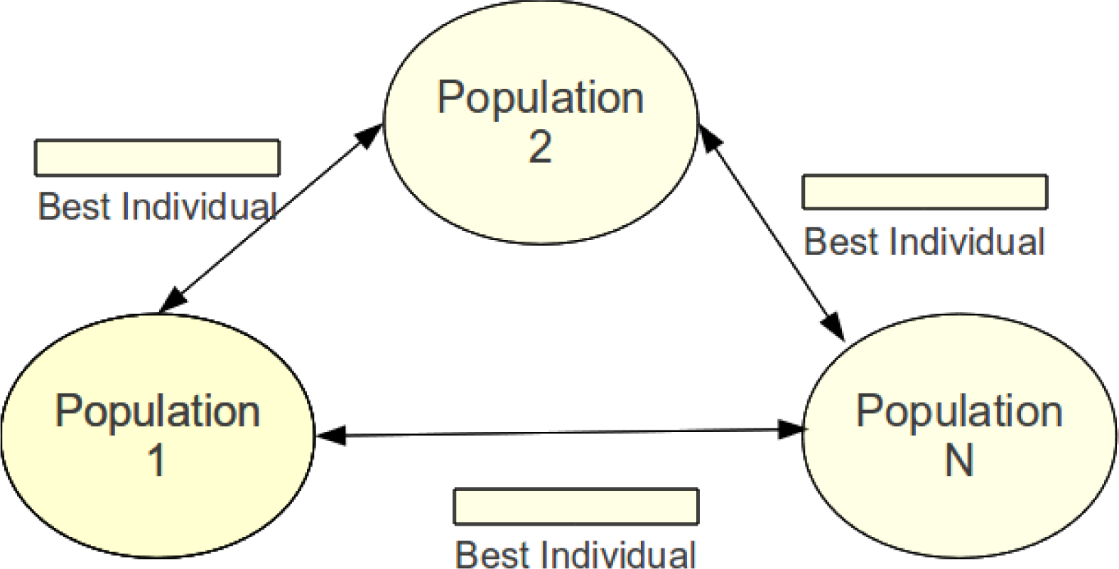
The details on how the algorithm performs the selection of the individuals selected to be migrated and the ones to be replaced is analyzed in detail in Section 4.3. Regarding the migration topology, all the islands communicate with each other in a collective manner, as is depicted in Figure 1.
3.2.2. Population Distribution in the Cluster
Since the available architecture is a heterogeneous grid of computers, it is obvious that the time to complete a generation during the run will be different on each computer [35]. As the distributed populations perform a collective communication broadcasting to individuals, the global performance of the algorithm would be injured if the fastest machines had to wait for the slower ones, wasting computing resources. In order to ameliorate this fact, the decision of setting different population sizes has been taken. Slower or overloaded machines will process less individuals, allowing these processes to require a shorter time to complete a generation. Therefore, during the collective communications, the waiting time for the synchronization will be reduced. Obviously, this approach is the same as increasing the predefined population size in the more powerful machines.
The question that arises from this policy is: how much should the size of the population be decreased/increased? The answer can be obtained empirically by measuring the time for one generation on each machine and obtaining the fraction between the fastest/slowest and the other time measurements. For example, if the time of Machine1 is double that of Machine2, the population size for Machine1 should be half (or the population size for Machine2 should be doubled).
Therefore, a communication step must be performed at the beginning of the algorithms: the root process (rank 0) is the reference, so each process with its corresponding GPU performs the evaluation of the same individual (i.e., all variables selected) and waits for the message from the root process, indicating how much it took to perform the evaluation. Then, each process computes the number of individuals as:
3.2.3. Optimizing the Computation of the Population Fitness
The implementation presented by [12] had to be adapted in order to use several GPUs within the same node. To do so, several functions from the NVIDIAlibrary have to be called, as is described in [36], to set the desired GPU by each process. For each time the KNN function is called, the whole reference dataset has to be copied to the GPU memory to compute the distances. Therefore, during the evaluation of the whole population, this process has to be repeated as many times as the number of individuals with the possibility of creating an overhead time that could be avoided, since a process will not use other GPUs than the one selected and the reference dataset is the same. The implementation of the function was modified, so that the complete population was given to the mex-function, which computes the KNN neighbors. Thus, the kernels, when computing the distances just have to accumulate or not accumulate a distance in a certain dimension depending on the value of the gene in the chromosome.
However, the implementation splits the queries to fit in the GPU memory, and this depends in the dimension of the dataset, performing a “memcopy” from the host to the device for each split. Therefore, the higher the dimension of the problem is, the longer it will take to compute the distances.
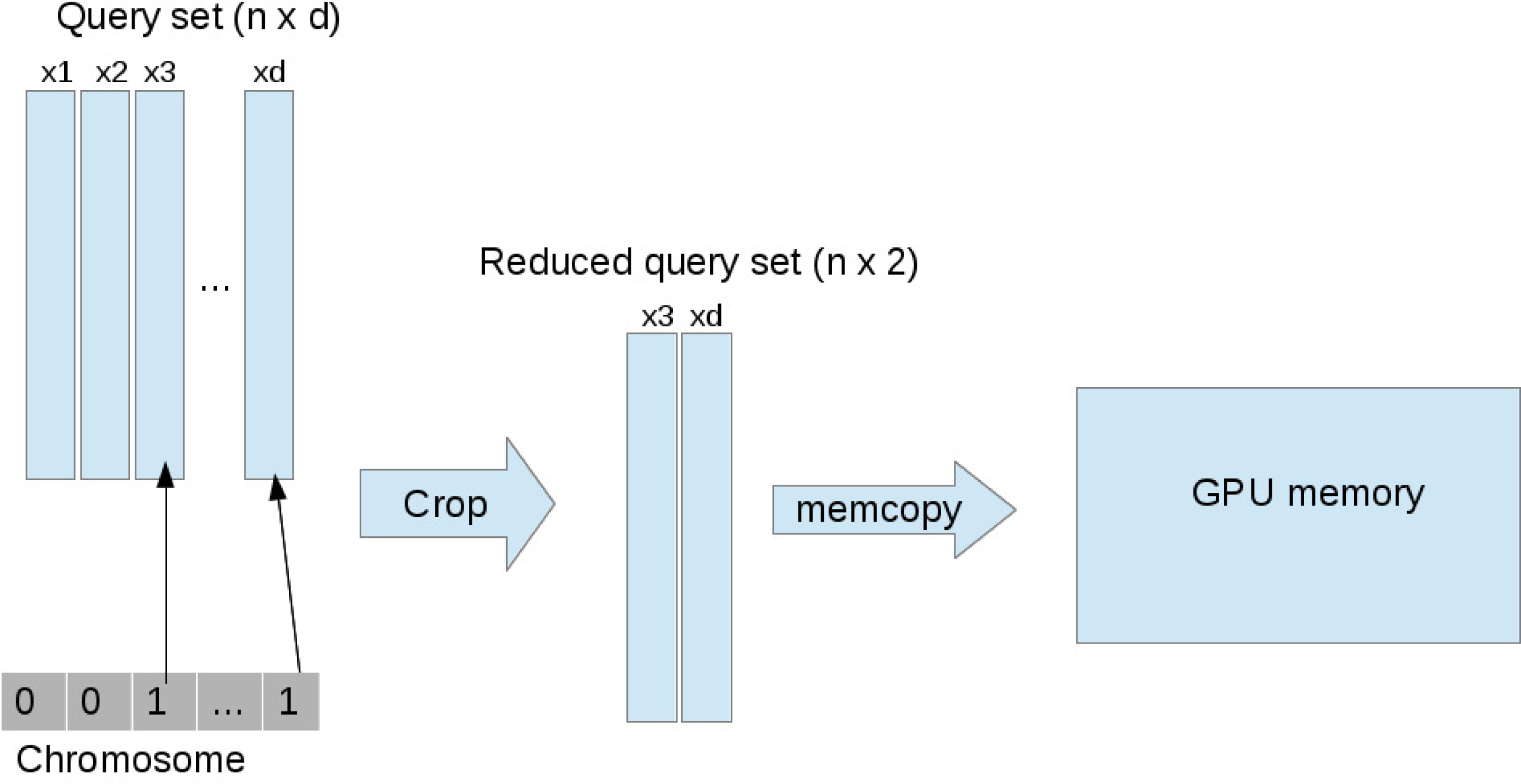
In this paper, this computation has been optimized, as the dimension of the dataset defined by each chromosome is different. For example, a chromosome that encodes a selection of just two variables does not need the other d − 2 variables. Therefore, the function distance computation function is called as many times as there are individuals, but cropping the dimensionality of the input vectors on each call to match the variable selection encoded on each chromosome. This process is depicted in Figure 2 with a chromosome that encodes a solution with two variables.
This cropping is easily performed in MATLAB, due to its efficient matrix operations. Therefore, the computation of the fitness for individuals with a low number of variables becomes much faster, as the KNN function does not have to split the query to iterate through all the dimensions of the dataset.
This reduction in time is much higher than the one obtained by reducing the number of calls to select the GPU and to perform the copy of the reference set to the GPU memory.
4. Experiments
This section shows the performance of the proposed algorithm when compared to previous approaches using small and large datasets. Afterwards, an analysis of the migration policy chosen is made.
4.1. Cluster Architecture
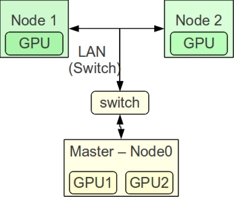
The cluster that was configured had the components described below that were interconnected, as Figure 3 shows.
- (1)
One master node with two GPUs:
Model name : (26) Intel(R) Core(TM) i7 CPU 930 @ 2.80 GHz—cache size: 8192 KB
CPU cores: 4; siblings: 8
Graphics processor: GeForce GTS 450—CUDA cores: 192
Memory: 1024 MB; memory interface: 128-bit
Bus Type: PCI Express x16 Gen1 - PCI-E Max link speed: 2500
- (2)
Two Local network node with one GPU:
Model name: (23) Intel(R) Core(TM)2 Quad CPU Q9550 @ 2.83 GHz—cache size: 6144 KB
CPU cores: 4; siblings: 4
Graphics processor: GeForce 9800 GTX — CUDA cores: 128
Memory: 512 MB; memory interface: 256-bit
Bus type: PCIExpress x16 Gen2; PCI-E max link speed: 5000
Model name: (15) Intel(R) Core(TM)2 Quad CPU Q6600 @ 2.40 GHz—cache size: 4096 KB
cpu cores: 4; siblings: 4
Graphics processor: GeForce 8400 GS—CUDA cores: 16
Memory: 512 MB; memory interface: 64-bit
Bus type: PCIExpress x16; PCI-E max link speed: not available
4.2. Comparison with Previous Approaches
This section will analyze the performance and behavior of the proposed algorithm. First, small datasets are compared with a previous work; afterwards, the algorithm is applied to a large real-world dataset.
4.2.1. Small Datasets
The algorithm is compared with the approach presented in [37], which is a previous parallel version of the algorithm implemented in a regular cluster. For the sake of a fair comparison, the stop criteria will be the same: execution time. In [37], the time limit is set to 600 s, based on studies and recommendations from the industry arguing that that is the maximum time that an operator is willing to wait to see a solution.
The same population sizes were used (50,100 and 150), and the datasets processed were: (1) The Tecator dataset [38]: The Tecator dataset aims at performing the task of predicting the fat content of a meat sample on the basis of its near-infrared absorbance spectrum. The dataset contains 215 useful instances for interpolation problems, with 100 input channels and 3 outputs, although only one is going to be used (fat content). (2) The Anthrokids modified dataset [39]:This dataset consists of several measures to predict a child’s weight. It has 1019 instances and 55 variables.
The results are shown in Table 1. As the table reflects, the performance of the proposed algorithm is not impressive in comparison with the previous algorithm. In fact, it does not outperform the previous approach. However, it is remarkable that the difference between the solutions is not too big, and in some cases, the new algorithm outperforms the previous one, demonstrating that the proposed approach is a good algorithm. The reason because the previous algorithm obtains, in general, better solutions for these datasets is because the GA is able to generate more populations, due to the pre-calculation of the distance matrix, as it was described in Section 2.
4.2.2. Large Datasets
The analysis of the previous results might discourage the use of GPUs instead of using a pre-calculation of the distances; however, when the dataset starts becoming a little bit bigger, this second approach is not possible any more. The reason is because the application runs out of memory, so to use a cluster of GPUs, it is not a matter of performance in time or quality results, it is a matter of being able to provide a solution.
As an example, part of the dataset provided by the Spanish Institute of Statistics (Instituto Nacional de Estadística (INE)) that contains data about marital dissolutions in Spain is used. Several problems arise from this data, and one of them is predicting the dissolution process length, which is translated into the regression problem.
The data to be used consists of 19,967 input samples of 20 variables, which is divided into training (of 15,385) test (4568) sets. The size of the training set is too big to pre-calculate the distance matrix used in previous approaches [37].
The proposed approach is executed during 600 s using the same configuration of the previous section (detailed in Section 3.1), being able to finish only one generation, with 50 individuals providing a DT value of 0.001642 using 9 variables. Due to the high memory requirements, one of the computers with the oldest GPU model was delaying the other two, because of the synchronization step in the migration. Therefore, the experiments are repeated only with two nodes instead of three. The performance increases significantly, allowing the algorithm to evolve a mean of 7.6 generations, obtaining a DT value of 0.001589 using only 4 variables.
To test the validity of the selection provided, a model (a radial basis function neural network with 15 neurons) is designed using the methodology proposed in [40] without local search optimization. The experiments are done using all the variables and using the ones selected by the algorithm, obtaining the results shown in Tables 2 and 3. The approximation errors provided by the neural networks prove how critical the necessity of performing variable selection before modeling a real world problem is. The network maintains a good generalization capability, as the differences between the test error and the training error are small.
4.3. Comparison Between Different Migration Policies
Another experiment carried out consists of a comparison of several approaches regarding how the communication between the islands is performed. In order to isolate as much as possible the effect of the migration parameters, the seeds of the random function used on each run is the same, so that the unique element that could modify the results is the migration step. The setting for the experiments is:
Send policy:
Send best (SB): selects the best individual of the current population;
Send random (SR): selects a random individual of the current population.
Acceptance policy:
Always accept (AA): always includes the incoming individuals to the population;
Accept if different (AiD): includes the individuals if they fulfill a predefined criterion.
Replacement policies:
Replace worst (RW): substitutes the worst individual by the incoming one.
Communication topology:
fully connected (send to all, receive from all).
Communication frequency:
synchronous fixed rate each 5 generations.
Regarding the send policy, the two selected options are considered, as are the most popular in the literature. The acceptance policy consists of always accepting the incoming individuals or only accepting them if they are different from the best individual in the population. In the implementation, an individual i⃗ = i1,i2, ..., id with ik ∈ 0, 1 is considered different from another individual if the Hamming distance between them is not higher than d/2.
As the tackled problem requires huge computational effort, only the worst individual replacement policy is chosen with the aim of converging to a good solution fast. Other approaches could consider other replacement policies.
4.3.1. Diversity of the Population
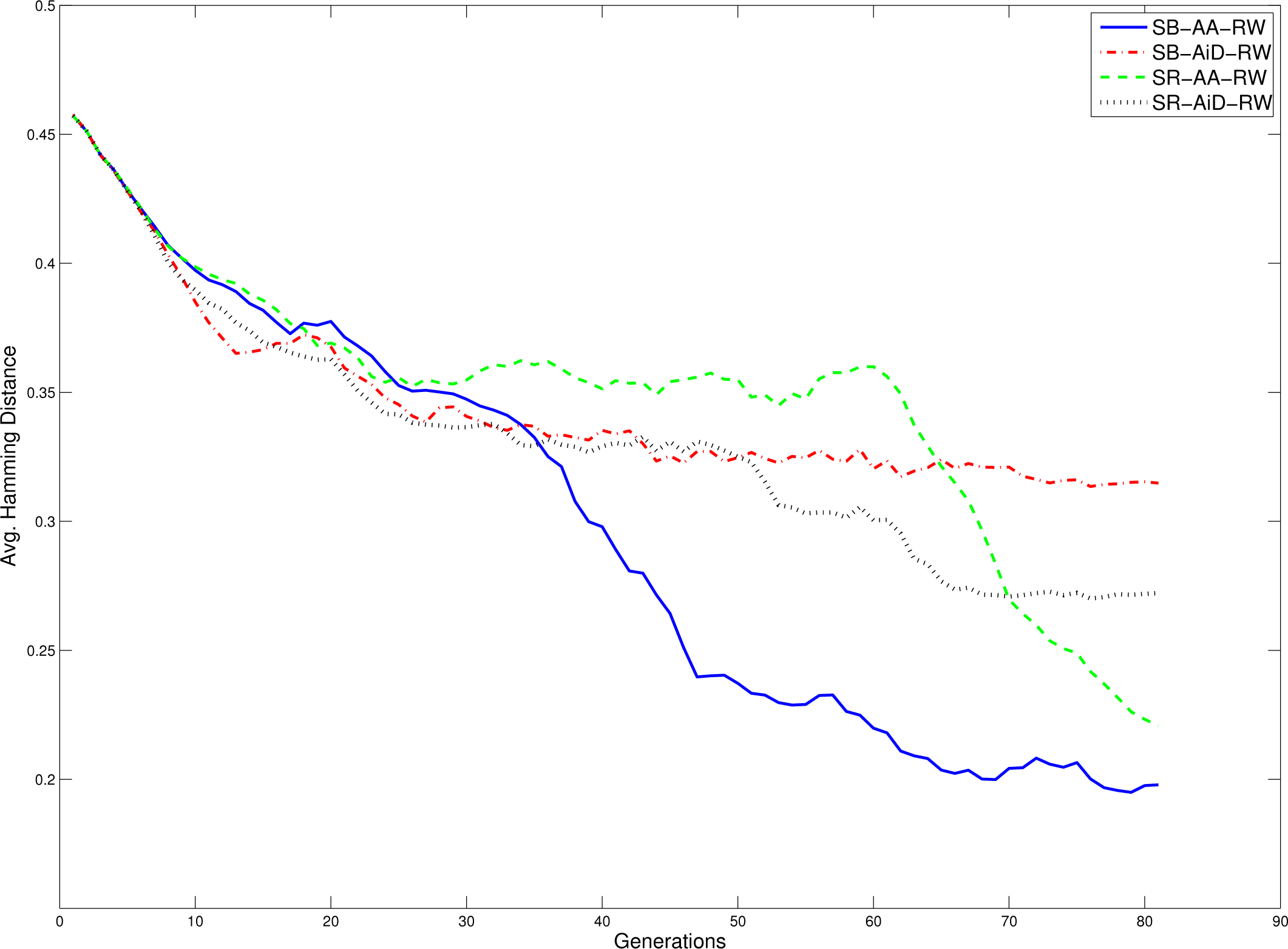
The value of the average Hamming distance between each pair of chromosomes is chosen to be the metric that determines the diversity of the population. For each run, the evolution of this parameter is recorded and, then, the average of the evolutions is computed; these values are graphically depicted in Figure 4. It is easy to see how the population maintains diversity when the conditional acceptance criterion is applied, and the configuration, SB-AA-RW, is the one that has less diversity in the population, confirming previous results.
4.3.2. Accuracy and Robustness
The reduction of the diversity by not using a conditional acceptance criterion could seem a disadvantage; however, as Table 4 shows, it is totally the opposite case, because it allows the algorithm to exploit the less divergent individuals more and to achieve better performance. This table also shows that the use of the conditional criterion does not affect the final result at all.
5. Conclusions
In this paper, we present a new algorithm that takes advantage of new high performance computing technologies. The main novelty is the use of a cluster, where the nodes have graphical processing units to compute the fitness function efficiently; this is a cluster of a cluster of GPUs. Another important contribution is the analysis of several migration policies, showing their influence on population diversity and result robustness. The performance of the algorithm for small datasets is acceptable when compared with previous methods, plus it is able to provide good results in a reasonable time. Even when the size of the dataset becomes too large, the proposed algorithm is able to provide a good solution, in contrast to the previous approach, which is not able to provide any.
Acknowledgments
This work was supported in part by the Consejería de Innovación, Ciencia y Empresa of the Spanish Junta de Andalucía, under Project TIC2906 and in part by the Spanish Ministry of Science and Innovation under Project SAF2010-20558.
Author Contributions
A. Guillén and L.J. Herrera have lead the ellaboration of the paper through all the stages. The rest of the authors have cooperated in the writting and revision of the paper.
Conflict of Interest
The authors declare no conflict of interest.
References
- Bellman, R. Adaptive Control Processes—A Guided Tour; Princeton University Press: Princeton, NJ, USA, 1961. [Google Scholar]
- Herrera, L.; Pomares, H.; Rojas, I.; Verleysen, M.; Guillén, A. Effective Input Variable Selection for Function Approximation. In Artificial Neural Networks—ICANN 2006, Proceedings of 16th International Conference, Athens, Greece, 10–14 September 2006; Part I. pp. 41–50.
- Liitiäinen, E.; Corona, F.; Lendasse, A. On the curse of dimensionality in supervised learning of smooth regression functions. Neural Process. Lett 2011, 34, 133–154. [Google Scholar]
- Shannon, C.E. A mathematical theory of communication. Bell Syst. Tech. J 1948, 27, 379–423. [Google Scholar]
- Pi, H.; Peterson, C. Finding the embedding dimension and variable dependencies in time series. Neural Comput 1994, 6, 509–520. [Google Scholar]
- Eirola, E.; Liitiäinen, E.; Lendasse, A.; Corona, F.; Verleysen, M. Using the Delta Test for Variable Selection. Proceedings of the ESANN 2008, European Symposium on Artificial Neural Networks, Bruges, Belgium, 23–25 April 2008; pp. 25–30.
- Eirola, E. Variable Selection with the Delta Test in Theory and Practice, Master’s Thesis, Helsinki University of Technology, Espoo, Finland. 2009.
- Liébana-Cabanillas, F.J.; Nogueras, R.; Herrera, L.J.; Guillén, A. Analysing user trust in electronic banking using data mining methods. Expert Syst. Appl 2013, 40, 5439–5447. [Google Scholar]
- Del Moral, R.G.; Guillén, A.; Herrera, L.J.; Cañas, A.; Rojas, I. Parametric and Non-Parametric Feature Selection for Kidney Transplants. Proceedings of The International Work-Conference on Artificial Neural Networks (IWANN), Tenerife, Spain, 12–14 June 2013; pp. 72–79.
- Liitiäinen, E.; Verleysen, M.; Corona, F.; Lendasse, A. Residual variance estimation in machine learning. Neurocomputing 2009, 72, 3692–3703. [Google Scholar]
- Jones, A.J. New tools in non-linear modeling and prediction. Comput. Manag. Sci 2004, 1, 109–149. [Google Scholar]
- Garcia, V.; Debreuve, E.; Barlaud, M. Fast k Nearest Neighbor Search Using GPU. Proceedings of the CVPR Workshop on Computer Vision on GPU, Anchorage, AK, USA, 23–28 June 2008.
- Source code for computing KNN using GPU. Available online: http://www.i3s.unice.fr/~creative/KNN/ (accessed on 13 October 2013).
- David, M. Mount and Sunil Arya ANN: A Library for Approximate Nearest Neighbor Searching. Available online: http://www.cs.umd.edu/mount/ANN/ (accessed on 13 October 2013).
- Obaid, O.I.; Ahmad, M.; Mostafa, S.A.; Mohammed, M.A. Comparing performance of genetic algorithm with varying crossover in solving examination timetabling problem. J. Emerg. Trends Comput. Inf. Sci 2012, 3, 1427–1434. [Google Scholar]
- Goldberg, D.E. Genetic and evolutionary algorithms come of age. Commun. ACM 1994, 37, 113–119. [Google Scholar]
- Jong, K.A.D. Evolutionary Computation—A Unified Approach; MIT Press: Cambridge, MA, USA, 2006. [Google Scholar]
- Wang, L.; Kazmierski, T. VHDL-AMS Based Genetic Optimization of a Fuzzy Logic Controller for Automotive Active Suspension Systems. Proceedings of the 2005 IEEE International Behavioral Modeling and Simulation Workshop, San Jose, CA, USA, 22–23 September 2005; pp. 124–127.
- Zhang, J.; Li, S.; Shen, S. Extracting Minimum Unsatisfiable Cores with a Greedy Genetic Algorithm. In AI 2006: Advances in Artificial Intelligence, Proceedings of 19th Australian Joint Conference on Artificial Intelligence, Hobart, Australia, 4–8 December 2006; pp. 847–856.
- Maximum wait time for group policy scripts. Available online: http://technet.microsoft.com/enus/library/cc940027.aspx (accessed on 1 December 2013).
- Minimum acceptable timeout value. Available online: https://developer.apple.com/library/ios/DOCUMENTATION/UIKit/Reference/UIApplicationClass/Reference/Reference.html (accessed on 1 December 2013).
- Maximum time an item in the search/bind cache remains valid. Available online: http://httpd.apache.org/docs/current/mod/mod_ldap.html (accessed on 1 December 2013).
- Alba, E.; Tomassini, M. Parallelism and evolutionary algorithms. IEEE Trans. Evol. Comput 2002, 6, 443–462. [Google Scholar]
- Guillén, A.; Rojas, I.; González, J.; Pomares, H.; Herrera, L.; Paechter, B. Boosting the Performance of a Multiobjective Algorithm to Design RBFNNs through Parallelization. In Adaptive and Natural Computing Algorithms, Proceedings of 8th International Conference, Warsaw, Poland, 11–14 April 2007; pp. 85–92.
- Guillén, A.; Pomares, H.; González, J.; Rojas, I.; Valenzuela, O.; Prieto, B. Parallel multiobjective memetic RBFNNs design and feature selection for function approximation problems. Neurocomputing 2009, 72, 3541–3555. [Google Scholar]
- Guillén, A.; Rojas, I.; González, J.; Pomares, H.; Herrera, L.; Paechter, B. Improving the Performance of Multi-Objective Genetic Algorithm for Function Approximation through Parallel Islands Specialisation. In AI 2006: Advances in Artificial Intelligence, Proceedings of 19th Australian Joint Conference on Artificial Intelligence, Hobart, Australia, 4–8 December 2006; pp. 1127–1132.
- Cantú-Paz, E. Efficient and Accurate Parallel Genetic Algorithms; Kluwer Academic Publishers: Norwell, MA, USA, 2000. [Google Scholar]
- Herrera, F.; Lozano, M. Gradual distributed real-coded genetic algorithms. IEEE Trans. Evol. Comput 2000, 4, 43–63. [Google Scholar]
- Chiwiacowsky, L.; de Velho, H.; Preto, A.; Stephany, S. Identifying Initial Conduction in Heat Conduction Transfer by a Genetic Algorithm: A Parallel Approach. Proceedings of the XXIV iberian Latin-American Congress on Computacional Methods in Engineering, Ouro Preto, Brazil, 29–31 October. 2003; pp. 180–195.
- Alba, E.; Troya, J.M. Influence of the migration policy in parallel distributed GAs with structured and panmictic populations. Appl. Intell 2000, 12, 163–181. [Google Scholar]
- Cantú-Paz, E. Migration Policies and Takeover Times in Parallel Genetic Algorithms. Proceedings of Genetic and Evolutionary Computation Conference, Orlando, FL, USA, 13–17 July 1999.
- Araujo, L.; Guervós, J.J.M. Diversity through multiculturality: Assessing migrant choice policies in an island model. IEEE Trans. Evol. Comput 2011, 15, 456–469. [Google Scholar]
- García-Sánchez, P.; Eiben, A.E.; Haasdijk, E.; Weel, B.; Guervós, J.J.M. Testing Diversity-Enhancing Migration Policies for Hybrid On-Line Evolution of Robot Controllers. Proceedings of the EvoApplications, Málaga, Spain, 11–13 April 2012; pp. 52–62.
- Miki, T.H.M.; Negami, M. Distributed Genetic Algorithms with Randomized Migration Rate. Proceedings of the IEEE Conference Systems, Man and Cybernetics, Tokyo, Japan, 12–15 October 1999; pp. 689–694.
- Alba, E.; Nebro, A.J.; Troya, J.M. Heterogeneous computing and parallel genetic algorithms. J. Parallel Distrib. Comput 2002, 62, 1362–1385. [Google Scholar]
- Guillén, A.; Arenas, M.G.; Herrera, L.; Pomares, H.; Rojas, I. GPU Cluster with MATLAB. Proceedings of the The 2011 International Conference on Parallel and Distributed Processing Techniques and Applications, Las Vegas, NV, USA, 18–21 July 2011; pp. 379–384.
- Guillén, A.; Sovilj, D.; Lendasse, A.; Mateo, F.; Rojas, I. Minimising the delta test for variable selection in regression problems. Int. J. High Perform. Syst. Archit 2008, 1, 269–281. [Google Scholar]
- StatLib: Data, Software and News from the Statistics Community. Available online: http://lib.stat.cmu.edu/datasets/tecator (accessed on 8 February 2014).
- Environmental and Industrial Machine Learning Group. Anthropometric study of US Children Carried Out in 1977. Available online: http://research.ics.tkk.fi/eiml/datasets.shtml (accessed on 8 February 2014).
- Guillén, A.; González, J.; Rojas, I.; Pomares, H.; Herrera, L.; Valenzuela, O.; Prieto, A. Improving clustering technique for functional approximation problem using fuzzy logic: ICFA algorithm. Neurocomputing 2007. [Google Scholar] [CrossRef]


| Dataset | Population | Measurement | seq. | parallel (np = 2) | parallel (np = 4) | pGPU (np = 4, nGPU = 4) |
|---|---|---|---|---|---|---|
| Anthrokids | 50 | Mean (DT) | 0.01278 (11.5 ×10⁻⁴) | 0.01269 (14.2 ×10⁻⁴) | 0.01204 (12.6 ×10⁻⁴) | 0.01587 (8.1 ×10⁻³) |
| 100 | Mean (DT) | 0.01351 (11.6 ×10⁻⁴) | 0.01266 (86.4 ×10⁻⁴) | 0.01202 (17.4 ×10⁻⁴) | 0.014553 (5.6 ×10⁻⁴) | |
| 150 | Mean (DT) | 0.01475 (12.1 ×10⁻⁴) | 0.01318 (11.2 ×10⁻⁴) | 0.01148 (9.9 ×10⁻⁴) | 0.01556 (12 ×10−4) | |
| Tecator | 50 | Mean (DT) | 0.13158 (7.9 ×10⁻⁴) | 0.14297 (7.7 ×10⁻³) | 0.13976 (7.8 ×10⁻³) | 0.123803 (3.7 ×10⁻³) |
| 100 | Mean (DT) | 0.13321 (3.1 ×10⁻³) | 0.13587 (2.4 ×10⁻³) | 0.13914 (8.6 ×10⁻³) | 0.132501 (3 ×10⁻³) | |
| 150 | Mean (DT) | 0.13146 (8.5 ×10⁻⁴) | 0.1345 (2.4 ×10⁻³) | 0.13522 (6.9 ×10⁻³) | 0.13197 (9.9 ×10⁻⁴) |
| Running Time | DT value (std) | # variables | # generations (std) |
|---|---|---|---|
| 600 s (3 nodes, 4 GPUs) | 0.001629 (2 ×10⁻⁴) | 9 | 1 (0) |
| 600 s (2 nodes, 3 GPUs) | 0.001592 (1 ×10⁻⁴) | 4 | 7.6 (0.5) |
| Train Error | Test Error | |
|---|---|---|
| with variable selection | 0.4846 | 0.5017 |
| without variable selection | 1.3086 | 1.3197 |
| Migration policy | DT value |
|---|---|
| SB-AA-RW | 1.668 ×10⁻³ (8.8 ×10⁻⁵) |
| SB-AiD-RW | 1.763 ×10⁻³ (1.1 ×10⁻⁴) |
| SR-AA-RW | 1.721 ×10⁻³ (1.3 ×10⁻⁴) |
| SR-AiD-RW | 1.721 ×10⁻³ (1.3 ×10⁻⁴) |
© 2014 by the authors; licensee MDPI, Basel, Switzerland This article is an open access article distributed under the terms and conditions of the Creative Commons Attribution license (http://creativecommons.org/licenses/by/3.0/).
Share and Cite
Guillén, A.; García Arenas, M.I.; Van Heeswijk, M.; Sovilj, D.; Lendasse, A.; Herrera, L.J.; Pomares, H.; Rojas, I. Fast Feature Selection in a GPU Cluster Using the Delta Test. Entropy 2014, 16, 854-869. https://doi.org/10.3390/e16020854
Guillén A, García Arenas MI, Van Heeswijk M, Sovilj D, Lendasse A, Herrera LJ, Pomares H, Rojas I. Fast Feature Selection in a GPU Cluster Using the Delta Test. Entropy. 2014; 16(2):854-869. https://doi.org/10.3390/e16020854
Chicago/Turabian StyleGuillén, Alberto, M. Isabel García Arenas, Mark Van Heeswijk, Dusan Sovilj, Amaury Lendasse, Luis Javier Herrera, Héctor Pomares, and Ignacio Rojas. 2014. "Fast Feature Selection in a GPU Cluster Using the Delta Test" Entropy 16, no. 2: 854-869. https://doi.org/10.3390/e16020854