On the Clausius-Duhem Inequality and Maximum Entropy Production in a Simple Radiating System

Abstract
: A black planet irradiated by a sun serves as the archetype for a simple radiating two-layer system admitting of a continuum of steady states under steadfast insolation. Steady entropy production rates may be calculated for different opacities of one of the layers, explicitly so for the radiative interactions, and indirectly for all the material irreversibilities involved in maintaining thermal uniformity in each layer. The second law of thermodynamics is laid down in two versions, one of which is the well-known Clausius-Duhem inequality, the other being a modern version known as the entropy inequality. By maximizing the material entropy production rate, a state may be selected that always fulfills the Clausius-Duhem inequality. Some formally possible steady states, while violating the latter, still obey the entropy inequality. In terms of Earth’s climate, global entropy production rates exhibit extrema for any “greenhouse effect”. However, and only insofar as the model be accepted as representative of Earth’s climate, the extrema will not be found to agree with observed (effective) temperatures assignable to both the atmosphere and surface. This notwithstanding, the overall entropy production for the present greenhouse effect on Earth is very close to the maximum entropy production rate of a uniformly warm steady state at the planet’s effective temperature. For an Earth with a weak(er) greenhouse effect the statement is no longer true.1. Introduction
In theories of thermomechanical behavior of a material continuum, conservation laws are on the whole not sufficient to constrain the constitutive equations that relate dependent fields. Further principles are called for in restricting possible relationships. Among the former, the second law of thermodynamics, particularly in the guise of the Clausius-Duhem inequality, plays a prominent role in thermomechanical theories [1,2]. Extremum principles may also be used as constraints, one of which, of more recent vintage, is but a hypothesis, the so-called maximum entropy production “principle” [3,4].
The Clausius-Duhem inequality is an entropy imbalance that defines an entropy production rate, a genuine creation of entropy, so it cannot be negative whenever irreversible processes take place within the system to which it is applied. It is this rate that is laid down in any investigation purporting to evince its maximum in some natural processes. In thermomechanics, admissible thermomechanical processes are defined as those solutions of the balance equations that also obey the Clausius-Duhem inequality. A notable feature of the latter is that it expressly accounts for radiation sources of energy and hence also of entropy. In typical presentations of a formal character, heating by radiation is regarded as arbitrarily prescribable, at least for the purposes of the constitutive theory [2,5,6]. Constitutive equations are derived in such a way that there is never a chance for the solutions of the balance equations to violate the Clausius-Duhem inequality. Such solutions are then said to be thermodynamically compatible. On the other hand, if the constitutive equations of a particular system are already known, the expectation is that the solutions of the balance equations ought to be thermodynamically compatible, whatever the radiation sources involved.
In the following exposition, instead of solving an energy balance equation to determine a material temperature field when the constitutive equations are known, we shall prescribe a thermal field, assuming that a specific temperature distribution can be maintained in a steady state by energy sources unidentified, in keeping with the spirit of Coleman and Noll’s paradigm [2]. We then calculate the radiation sources that follow from the temperature field and, by so doing, will be in a position to determine, if only indirectly, the rate of entropy production of the model.
2. The Clausius-Duhem Inequality
In thermomechanics of continua, a typical form of the energy balance reads [7]:
u denoting the specific internal energy, ρ the density of the material continuum, ɛ an internal source of energy, while Jq is typically a conductive heat flux; r is introduced to account for sources of energy due to radiation only. Astarita and Marrucci [7] highlight the role of r as “a quantity which—in principle—can be assigned at will: one may radiate as much energy as desired by controlling the temperature of the external radiation source, hence independently of the state of the material considered”.
When considering the entropy balance of the material continuum, the (volumetric) energy exchange r enters the balance as an entropy supply r/T [1,5,6,8]:
s stands for the specific entropy of matter, −Jq · N typically means the heat inflow through the system’s boundary whose field of outward normal vectors is N, while the density σm denotes the local rate of entropy production of all irreversible processes taking place in the material continuum occupying the volume dV. The entropy balance Equation (2) of a body is oblivious of the presence, in the same volume V, of any electromagnetic waves and their associated thermodynamical properties. The only coupling between radiation and matter is represented by energy supplied at the rate r. Radiant energy travelling (reversibly) across ∂V, changing thereby the entropy within the volume V, is not accounted for. Alongside the assumption Pm ≡ ∫V σmdV ≥ 0, relation (2) is known as the Clausius-Duhem inequality in thermomechanical theories, all of which take it for granted that the second law of thermodynamics requires the left-hand side of Equation (2) to be positive semidefinite [1,2,6].
In this essay, two plane-parallel layers of radiating matter, not in thermal equilibrium with each other, will serve as the prototype of a planet orbiting in a vacuum. The outer boundary of a planet is taken to be a surface where the density of the atmosphere can be neglected, with the consequent vanishing of the material fluxes through it. By further confining the analysis of the system to the steady-state version of Equation (2), we are left with the balance
Rate r can have in principle either sign, corresponding to emission or absorption of radiation. Because the Clausius-Duhem inequality exacts Pm to be positive definite, in a steady state r would have to be constitutively constrained [3]. On the other hand, we may conceive, as rational thermodynamicists ask us to do, arbitrary radiative energy sources r, among which some could only be balanced by an overall negative entropy production rate Pm, thus denying the unconditional validity of the Clausius-Duhem inequality. That a model of radiating matter may indeed be framed with such a property is one aim of the following lines. One way of avoiding the negative rates that arise in such a model—it may be revealed at this point—is by choosing only states with entropy supply rates close to or at their maximum values. A better resource is to treat the radiation field as part of the system and then extend the Clausius-Duhem inequality accordingly. We shall discuss both these means below.
3. The Model Defined
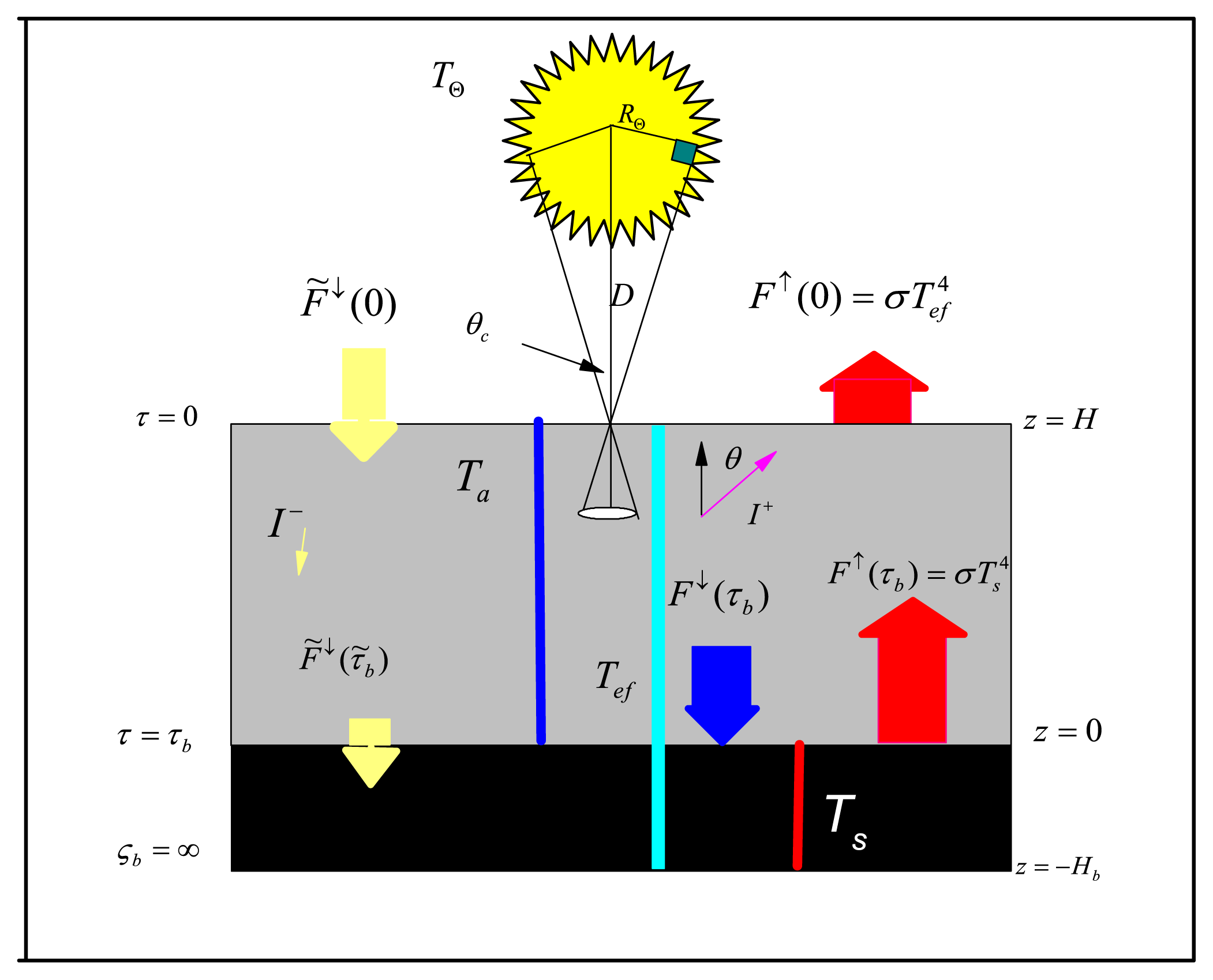
The model is based on the global energetics of a black planet subject to irradiation by a sun. Consider two contiguous horizontal layers of matter in vacuo, one on top of the other (a shallow atmosphere resting on a surface layer), irradiated by a hot external source (the sun) located at some distance aloft and, usually, at some average zenith angle θ⊚, see Figure 1. (For ease of drawing, θ⊚ has been taken to be zero, but in subsequent numerical calculations we shall use μ⊚ ≡ cos θ⊚ = 1/4, a value that enables us to take into account the fact that the emitting surface of a spherical, rotating planet is four times the area insolated by the sun.) The lower layer will be assumed to behave thermally as a blackbody, with no net exchanges of energy through its lowermost boundary. Overlying this black layer, and in contact with it, an atmosphere verges into the surrounding vacuum. This atmosphere we assume to be composed of what is known as semigray matter in astrophysics [10], meaning that the absorption coefficient of the atmosphere does not depend, except for an intermediate jump in its value, on the frequency of the electromagnetic waves involved in the energetic interactions between the radiation sources and the material layers. The layer is thus characterized by two absorption coefficients, one relating to the “shortwave” (solar) radiation of the hot source, and the other to the thermal (infrared) radiation of the relatively cold layers. To sanction such a spectral separation, the radiation of the exterior source has to be much hotter than the proper radiation of the cooler layers. For some further discussion of this model, I refer the reader to [9].
The source is assumed to remain forever at the fixed temperature T⊚. The temperatures Ta and Ts of the upper and lower layers, respectively, are allowed to take on different values, in accordance with the upper layer’s infrared opacity, as we shall see soon. The temperature “field” thus consists of two uniformly warm layers, with a temperature jump at the surface of contact between them. Their steady temperatures are to be maintained even, by material processes we need not know explicitly. All we ask of them is that they be somehow realizable, or at least imaginable for the purposes of our exemplary illustration. The temperatures obey local energy balances of the type of Equation (1), with suitable energy sources we will not specify, but with an energy supply by radiation that we shall be able to calculate explicitly from the given temperature distribution. If such a distribution turns out to satisfy the balance equations as well as the Clausius-Duhem inequality, by definition it constitutes a thermodynamic process [2]. The model, as is the case for Earth on average, stays continually in an overall steady-state, in which radiative fluxes of energy enter and leave the whole system at the same rate through the outward boundary, where the density of matter, ρ, vanishes together with the optical depth. Optical depth, τ, will be our variable of choice as the model’s spatial variable, following astrophysical practice. It is related to geometric distance, z, measured across the layers, by , with H representing the geometric thickness of the layer in question, and is gauged from a reference level for which z = 0. In Figure 1 it is seen that the reference level for the upper layer is sea level (the interface between both layers), while the optical depth of the lower layer, denoted by ς to preempt any confusion later on, refers to z = −Hb, with h being distance from that bottom: . k is the specific absorption coefficient already alluded to. The optical depth of the whole layer, a measure of the layer’s opacity, is just the value of τ at the reference level, τ (0) ≡ τb (or ςb = ∞ at h = 0). It reflects both the amount of absorbing matter in the layer and its specific capacity to absorb radiation. Since we deal with two different radiation regimes (two values of k), we distinguish symbols by using them either as just introduced, when they relate to the thermal regime, or by placing a tilde whenever the quantities refer to the shortwave domain. Thus, e.g., τ̃ or τ̃b refer to optical depth with respect to the (hot) shortwave radiation of the source. A further simplification is to assume a uniformly constant ratio between the absorption coefficients [10]: k̃/k = ε, with ε = 0 describing a wholly transparent upper layer to solar radiation.
As the infrared opacity (τb) of the upper layer will serve as a control parameter of the model (representing varying strengths of the greenhouse effect on a planet due to variable amounts of greenhouse gases), the layer’s uniform temperature and hence its emission is to be adjusted so as to maintain the energy balance of the system. This balance will be referred to a unit of area, as will also all the following total entropy production rates (like Pm). The (hot) radiative energy flux density arriving at the outer boundary of the model from the external source we will denote by F̃↓(0), while the (cold) radiation flux density leaving the system through the same boundary will be written as F↑(0). The model’s steady-state energy balance can then be expressed simply as F̃↓(0) = F↑(0). A measure of the model’s unvarying overall thermal level is its effective temperature, Tef, defined by , σ being the Stefan-Boltzmann constant. It defines the temperature a blackbody would have to be at in order to emit exactly the given energy flux density, F↑(0). Because we allow the two model layers to take on different if uniform temperatures, Ta and Ts, neither agrees with Tef, unless we happen to be dealing with one of the limiting cases: (1) Ta = Ts; (2) the upper layer is entirely transparent (τ̃b = τb = 0), so it cannot modify the radiation emitted by the lower layer, entailing Ts = Tef; or (3) the upper layer is thermally opaque (τb → ∞), in which case the lower layer cannot contribute to the radiation emitted into vacuum, so necessarily Ta = Tef. These limits follow from , together with the solution of the radiative transfer equation for the upwelling thermal radiation, resulting in the following relation between the three temperatures so far introduced (cf. Equation (9) at τ = 0, after integrations furnishing the flux density):
Here, E3(τb) is the exponential integral of order 3, the n-th order being defined as . It is a function of the upper layer’s infrared opacity. For a thermally transparent layer (no greenhouse gases), we have 2E3(0) = 1; for a thermally black layer, E3(∞) = 0, and Equation (4) is rendered simply as Ta = Tef.
The basic quantity in the phenomenological theory of radiation transport is the radiance, Iν [10,11]. Besides frequency ν, it is a function of position, time and direction. The model’s horizontal uniformity implies that the steady-state radiances will be functions of only the optical depth τ and an angular coordinate that fixes the direction of propagation of a ray. It is common to use the direction cosine μ ≡ cos θ ∈ [−1, 1], where θ ∈ [0, π] denotes the polar angle of a ray with respect to the outward normal unit vector. We thus write the steady monochromatic radiance as Iν(τ, μ). It represents the radiant energy flowing, in a unit of time, through an element of area oriented at an angle θ, within an element of solid angle around the propagation direction, and encompassing an infinitesimal interval of frequencies ν (or, equivalently, of wavelengths λ). We obtain the quantity of interest, i.e., the energy supply, r = −dF/dτ, as the divergence of the frequency-integrated radiative flux density, , defined as the first directional moment of the radiance in μ-space. The net energy gain we shall write as F = F↓−F↑, aswe need to distinguish downwelling and upwelling energy flux densities, defined in our model configuration by and , respectively. (Symbols devoid of the index ν are to be understood as quantities that have been integrated over all possible frequencies of electromagnetic waves, with the implication that the slight modifications due to contributions in the shortwave or longwave tails thereby encompassed are negligible). Likewise, we need to distinguish the flux densities of the two broadband spectral domains discussed above. F̃ and F denote the shortwave and thermal radiative flux densities, respectively, as already introduced in the global energy balance above. It must be noted, however, that F̃ is a function of τ̃ = ετ. Deriving this function with respect to infrared optical depth leads to r̃(τ) = −dF̃/dτ = −d F̃/dτ̃ = r̃(τ̃).
The radiances Iν are determined by solving the equation of radiative transfer [11], which in our optical space with scattering excluded becomes [10,12]:
Jν(μ, τ ) describes, in thermodynamical terms, a net nonequilibrium flux of energy between a ray of direction θ and a volume element of matter radiating isotropically at local temperature T(τ ). The change dIν of radiance is due to absorption and emission of radiation of the same frequency. Bν, the source of monochromatic radiance issuing from matter in local thermodynamic equilibrium, is given by Bν(τ) =
 [T(τ )], where
is Planck’s function, the spectral distribution of which we write as
(T) =
[T(τ )], where
is Planck’s function, the spectral distribution of which we write as
(T) =
 /(ehν/kT −1), with the shorthand
in which the constants have their customary meanings: h is Planck’s constant, k Boltzmann’s, and c0 represents the speed of light through empty space. Due to different boundary conditions, in solving Equation (5) we must treat the radiance fields separately. We mark quantities associated with downwelling radiances (for which μ < 0) with a minus sign, attaching a + to those corresponding to upwelling radiances (μ > 0), the arrows being reserved for corresponding vertical flux densities, as depicted in Figure 1.
/(ehν/kT −1), with the shorthand
in which the constants have their customary meanings: h is Planck’s constant, k Boltzmann’s, and c0 represents the speed of light through empty space. Due to different boundary conditions, in solving Equation (5) we must treat the radiance fields separately. We mark quantities associated with downwelling radiances (for which μ < 0) with a minus sign, attaching a + to those corresponding to upwelling radiances (μ > 0), the arrows being reserved for corresponding vertical flux densities, as depicted in Figure 1.
The energy supply to a material element due to the radiation field, r, can now be calculated by integrating the radiative transfer Equation (5) with respect to frequency and direction, whereby the time-independent directional derivative μdIν/dτ becomes the divergence of the flux density: (the prime indicating d/dτ). The energy supply in each of both spectral regimes may in turn be divided into two partial supplies, r+ and r−, owing to the interaction with either the upwelling radiance field or the downwelling radiation, respectively. Thus, r(τ) = r+(τ) + r−(τ ), with the definitions
We next turn to the evaluation of energy supplies in the two different spectral regimes.
3.1. Energy Supply from Shortwave Radiation
In choosing well-separated radiation regimes, the radiance incident from the (hot) external source is barely reinforced by emission at room temperatures, and consequently we can neglect in Equation (5) the source function Bν for shortwave radiation, so that . As the external spherical source is assumed placed afar (at distance D), the radiation impinging on the top of the upper layer (where τ̃ = τ = 0) is made up of rays confined within a cone of half-angle θc = cos−1 μc, a cone subtending the external source that we may picture inverted with its vertex at the top of the layer (cf. Figure 1). The solution of the radiative transfer Equation (5) for the downwelling monochromatic radiance is readily found to be , the boundary condition being for μ within a small solid angle around the zenith direction −μ⊚ (= −1 in Figure 1), and zero otherwise. With shortwave radiance thus available as a function of optical depth, we determine the energy supply Equation (6) to be
where the variable μ within the slender cone of incident radiances has been replaced by the axial direction cosine −μ⊚, so that the μ-integration may be reduced to the configuration of Figure 1, yielding 1 − μc, which is close to , an excellent approximation for the envisaged distances D >> R⊚, where R⊚ is the radius of the spherical source. The impinging shortwave irradiance, Q0, is the source’s emission , diluted by the factor (R⊚/D)2. As pointed out above, in terms of infrared optical depth τ, the energy supply Equation (7) is slightly modified to read:
3.2. Energy Supply from Infrared Radiation
To calculate the rates of infrared energy supply, we integrate the radiative transfer Equation (5) for different boundary conditions. Because temperature is uniform, the upper layer radiances are found to be
We note that only a negligible amount of infrared radiation enters a planet from space, hence . With these radiances the energy supplies Equation (6) are found to be and . The total energy supply to the atmosphere is the sum of both rates and the shortwave energy supply Equation (8),
For the lower layer with its infinite optical depth, we solve Equation (5) with the upper boundary condition , obtaining for the radiances within the layer and . This gives r+(ς) = 0 and . Also, as is apparent, r̃−(σ̃) = Q0e−τ̃b/μ⊚e−σ̃/μ⊚, so that, as for the upper layer, r̃−(ς) = εsr̃−(σ̃). Hence,
In what sense are the supplies (11) and (12) arbitrary? Well, we may vary D, R⊚, τb, τ̃b (ε), and the temperatures T⊚, Ts or Ta. Even fixing the parameters of the external source, we may vary the independent model parameters, always heeding the condition (4). If we further fix the optical depths of the upper layer, by Equation (4) either Ts or Ta remains arbitrary. Once Ts or Ta is fastened, the remaining temperature is no longer free, and we have a certain thermodynamic process (a putative solution of the balance equations) which is attended by a steady, unspecified, material net flux density through the interface at z = 0, which we denote as Fm. Different pairs of temperatures are of course attended by correspondingly adjusted fluxes Fm. So, leaving Ts at our discretion, we have a model to calculate indirectly entropy production rates and fluxes Fm as a function of the blackbody temperature of the surface layer. We go on to show this.
3.3. Material Entropy Production in the Steady State
We proceed to calculate the integrated supply of entropy from the right-hand side of Equation (3), in the optical space of our layers. Towards that end, we split the integration domain and first calculate the entropy supply of the upper layer, , followed by that of the lower layer, (more easily solved by bearing in mind the relation between supplies and flux divergences, e.g., d F̃↓/dσ̃ = −r̃−(σ̃)), eventually adding them up to get an expression that allows us to determine (if only indirectly) the steady rate Pm. We find
From their definitions we have F̃↓(τ̃b) = F̃↓(0)e−τ̃b/μ⊚ and . In global (radiative) equilibrium, F̃↓(0) = Q0μ⊚ = F↑(0), so that by taking into account Equation (4), Equation (13) can be rewritten as a simple bilinear product of a flux and a temperature difference:
We note that in our posited steady state the total net radiation flux density, F̃↓(τ̃b) + F↓(τb) − F↑(τb), is balanced by the (implicit) net material flux density between the layers, Fm. We thus have an expression delivering the steady entropy production rates in terms of both optical depths and the surface temperature Ts. By a slight abuse of notation, I write the right-hand side of Equation (14) as Pm(τ̃b, τb, Ts).
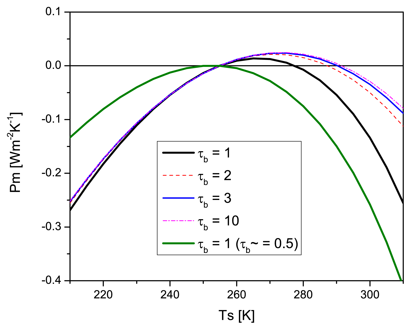
Figure 2 shows the rates Pm(τ̃b, τb, Ts) as a function of the surface temperature Ts, for four different values of the thermal optical depths and two values of τ̃b; in the visible domain the optical depth is chosen to be rather small, τ̃b = 0.084, a particular value corresponding to a rather transparent atmosphere [9]; the higher value of τ̃b = 0.5 reflects a rather polluted atmosphere (olive curve in Figure 2); τb = 1 may be thought of as the value associated with a moderate greenhouse, while τb = 3 already approaches a thermally opaque atmosphere, reflecting a strong greenhouse effect.
In evaluating the formulas illustrated in the figures the following values have been used: For the temperature of the external source we take the sun’s effective temperature, T⊚ = 5780 K; by removing our layers to a distance of roughly 1.195 astronomical units from our sun, and by choosing an average value for μ⊚ = 0.25 (appropriate to Earth as a swiftly rotating planet), the irradiation at the outer boundary amounts to the average absorbed power of Earth, or nearly 240 Wm−2. The resulting effective temperature is calculated to be Tef = 254.86 K.
Because Pm < 0 is forbidden by the Clausius-Duhem inequality, we conclude that the latter places a “constitutive” constraint on the net flux density at the interface, enforcing F̃↓(τ̃b) + F↓(τb) > F↑(τb), which translates into the statement that in a steady state the material energy fluxes Fm must be directed from the hotter lower layer to the colder upper one. This intuitively reasonable inference, albeit not inescapable as we shall discuss below, holds true for an interval (possibly reducing to a point, cf. the olive curve in Figure 2) of surface temperatures around that value of Ts for which the material entropy production rate is a maximum. Thus, by defining a “Clausius-Duhem interval” around the surface temperature of maximal radiative entropy supply rate, the validity of the Clausius-Duhem inequality is ensured. However, as will be shown shortly, by accounting for the irreversibility of radiative processes in the second law of thermodynamics, a less strict interpretation is allowed of, inasmuch as the entropy produced in the act of absorption and emission of radiation more than outweighs our model’s inferred (negative) material entropy production rates. We turn to consider this aspect next.
4. Entropy Production Due to Radiative Exchange of Energy
The exchange of energy by absorption and emission is a primary process in a planet’s energy budget. A summary of this aspect is all we are going to offer here. More details can be found in [9].
A homogeneous monochromatic ray of light or heat is, from a phenomenological standpoint, necessarily endowed with entropy. This is due to the fact that the natural electromagnetic waves it is composed of are subject to random fluctuations in phase, amplitude and direction [13]. The radiance Iν introduced above is an average over a spell long enough from the microscopic viewpoint but short-lived for the radiance to be ascertainable at a certain moment of time t. Iν is the main quantity to calculate the energy fluxes due to radiation. As to entropy fluxes, the corresponding entity is the monochromatic entropy radiance, Lν, a function of the monochromatic energy radiance Iν alone. It is defined by Planck’s well-known entropy formula [13],
where . The energy radiance Iν can also be expressed through Planck’s law as a temperature [13], , known in astrophysics as the monochromatic brightness temperature [12]. The monochromatic entropy radiance obeys the relation dLν/dIν = 1/Tν, first postulated to be valid out of thermodynamic equilibrium by Planck [13]; it may be interpreted as the Gibbs equation of the subsystem “beam of radiation” [14].
By virtue of this Gibbs-Planck relation we may set up, starting from Equation (5), a transfer equation for entropy radiance [15]. The result is an equation similar to Equation (5), with Iν replaced by Lν, and Bν(τ ) by Qν(τ, μ) = ν [Bν(τ )] +lν(τ, μ), the source of entropy radiance. In the latter, ν [Bν(τ )] is the isotropic part, while lν(τ, μ) ≡ lν [Bν(τ ), Iν(τ, μ)] is an anisotropic contribution that can be written as [16]:
In close correspondence to the previous definitions regarding radiant energy, we define the upwelling and downwelling flux densities of radiant entropy, , and , yielding as net gain of radiant entropy . Integrating the entropy radiance transfer equation with respect to frequency and directions yields , where σ* (τ ) represents the radiant entropy source at optical depth τ; as with radiant energy, we distinguish upgoing from downwelling entropy fluxes, and corresponding radiant entropy sources , expressible as
the total local source density of entropy radiation being . For the downwelling and upwelling fields we have the separate equations for entropy flux densities, and .
If in Equation (15) we insert the energy radiance of blackbody radiation at temperature T, i.e.,
(T), integration with respect to frequency yields
and a further integration with respect to direction leads to
. A neat proof that this relation is constitutively required by the second law of thermodynamics has been provided by [17].
Before proceeding, we flesh out the Clausius-Duhem inequality so as to encompass the radiation field as a thermodynamic system in its own right.
4.1. The Entropy Inequality for the Combined System of Matter and Radiation
It is known that in thermodynamic theories of linear constitutive equations, irreversible processes can be written as bilinear expressions in “fluxes” and “thermodynamic forces” (or “affinities”), the former being considered as the response to the latter. Phenomenologically, the interaction of a radiation field with (a continuum of) matter is no exception. Whenever a monochromatic ray of radiation, traveling in a specified direction through locally absorbing and emitting matter, is not in equilibrium with it, energy and entropy are transferred from one subsystem to the other across a temperature lapse, by virtue of which additional entropy is produced at a certain rate (as no macroscopic work is done). Entropy also grows when radiation energy is merely scattered about (as in conservative scattering), but we willfully have been ignoring this process. Exchange of energy (in a unit volume) is possible if the temperature of matter and the (brightness) temperature of the monochromatic ray differ. The entropy produced thereby may be given the classic bilinear form JνXν [14,18–20], where the thermodynamic flux is Jν (= Iν − Bν), while the difference of reciprocal temperatures, , is construed as the “driving force” of the irreversible exchange of energy. Since the radiation field consists of a spectrum of waves with different wavelengths, traveling from and into all directions at a point in space, the rate of local entropy production is the result of summing JνXν over all possible frequencies and directions, , and σr(x) ≥ 0 holds true always, the equality being effective only when the flux Jν vanishes together with the driving force Xν, so it indeed constitutes an entropy production rate in the very sense of the classical linear theory of irreversible thermodynamics. It reflects the fact that the radiative exchange in question is an irreversible process. A further integration of σr over a unit-area column of the optically active matter will then give the entropy production rate, Pr, of the composite system.
When considering the entropy balance of the entire system, consisting of matter as one subsystem, together with the coextensive fields of rays as further subsystems, the entropy supply in Equation (2) joins the source term of the entropy balance of the electromagnetic subsystem, Equation (17), to yield an expression [14,19–21] that resembles the general entropy inequality [5,22,23]:
where sr is the entropy density of the radiation field, and where the entropy flux density of the composite system now includes a contribution that is not of the classical constitutive form “heat over temperature” [22,23]: Js = (Jq/T ) − Φ*, the entropy flux density Φ* within the radiation continuum being defined exactly as the energy flux density, but with entropy radiance Lν replacing Iν. We need not deal with the contributions to the material entropy flux density Js, which more generally also comprehends exchanges of matter, nor discuss any of the various material production densities adding up to σm, as they are dispensable for our present purposes. All we shall need is the explicit radiation entropy production density in optical space, i.e., σr(τ) = r(τ )T−1(τ ) − σ* (τ ), in the simple setting of our model.
When considering the stationary balance of the total entropy of our model, Equation (18) shortens to
with the understanding that Pst = Pm + Pr, and Pr = ∫ σrdτ. Note that and, as we have not allowed for reflection of shortwave radiation, . The stationary global entropy production, Pst, is the sum of two global entropy production rates of different kinds: one owing to processes in the matter continuum, Pm, and the other due to the interaction between matter and the radiation fields, Pr. We stress our standpoint that the second law strictly enforces Pst ≥ 0, not Pm ≥ 0.
Setting aside the derivation of the rate of entropy production due to absorption and emission processes, for which I refer the reader to [9], let us here merely record the rate as it applies to our model:
The function η+(τb) is a rather involved integration arising from the anisotropic term, Equation (16); suffice it to say that it vanishes for τb = 0 and τb → ∞.
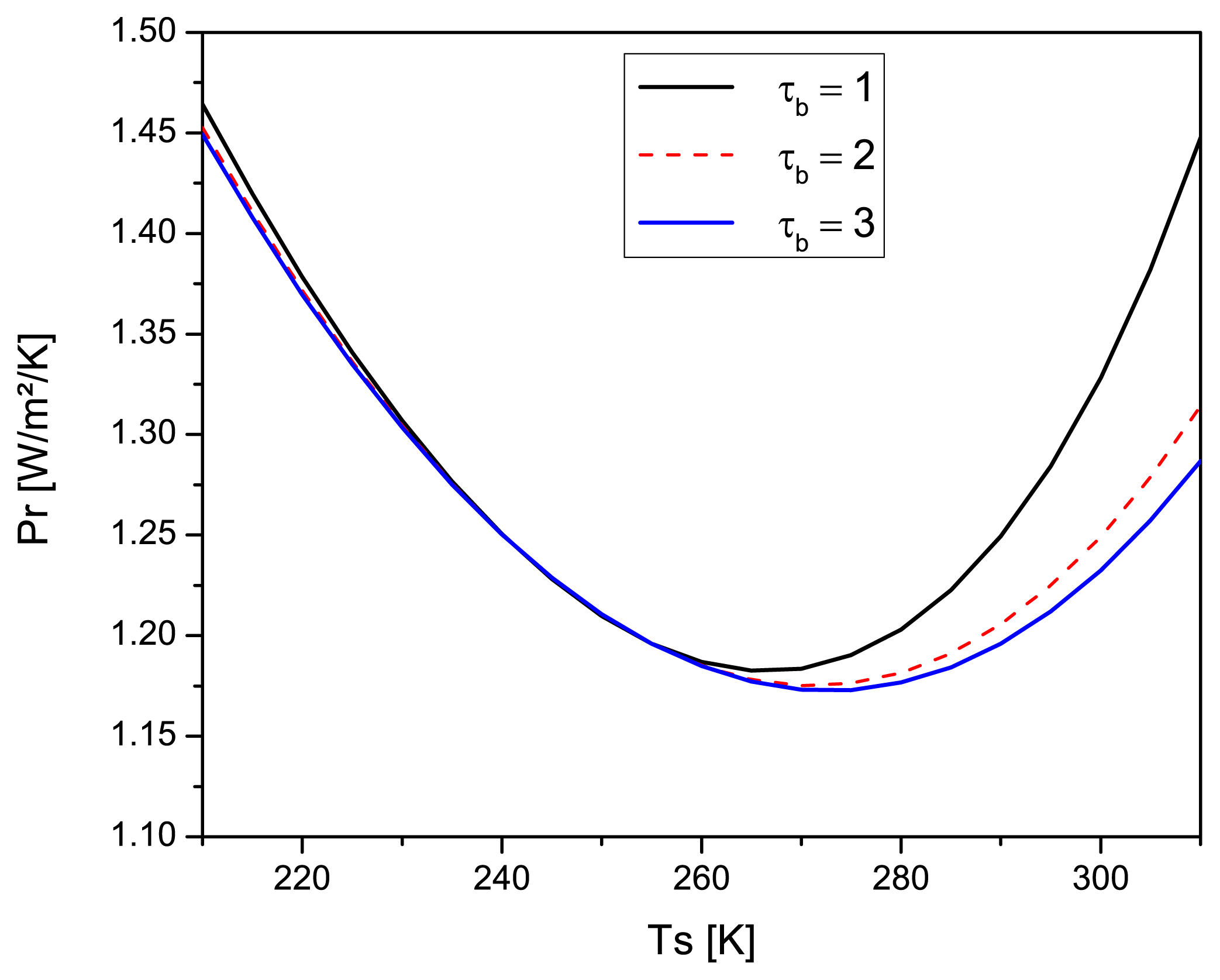
Figure 3 shows entropy production rates Pr(τ̃b = 0.084, τb, Ts), as a function of surface temperature and for three fixed values of the infrared optical depth. It can be seen that for each τb the rate achieves a minimum value, apparently at that surface temperature for which Equation (14) reaches a maximum at the matching fixed optical depth. An analytic proof of this numerical hint turns out to be rather cumbersome, due to the nonlinear function’s η+ dependence on Ts.
Finally, the total entropy production rate of the model in its steady state is obtained by summing Equations (13) and (20):
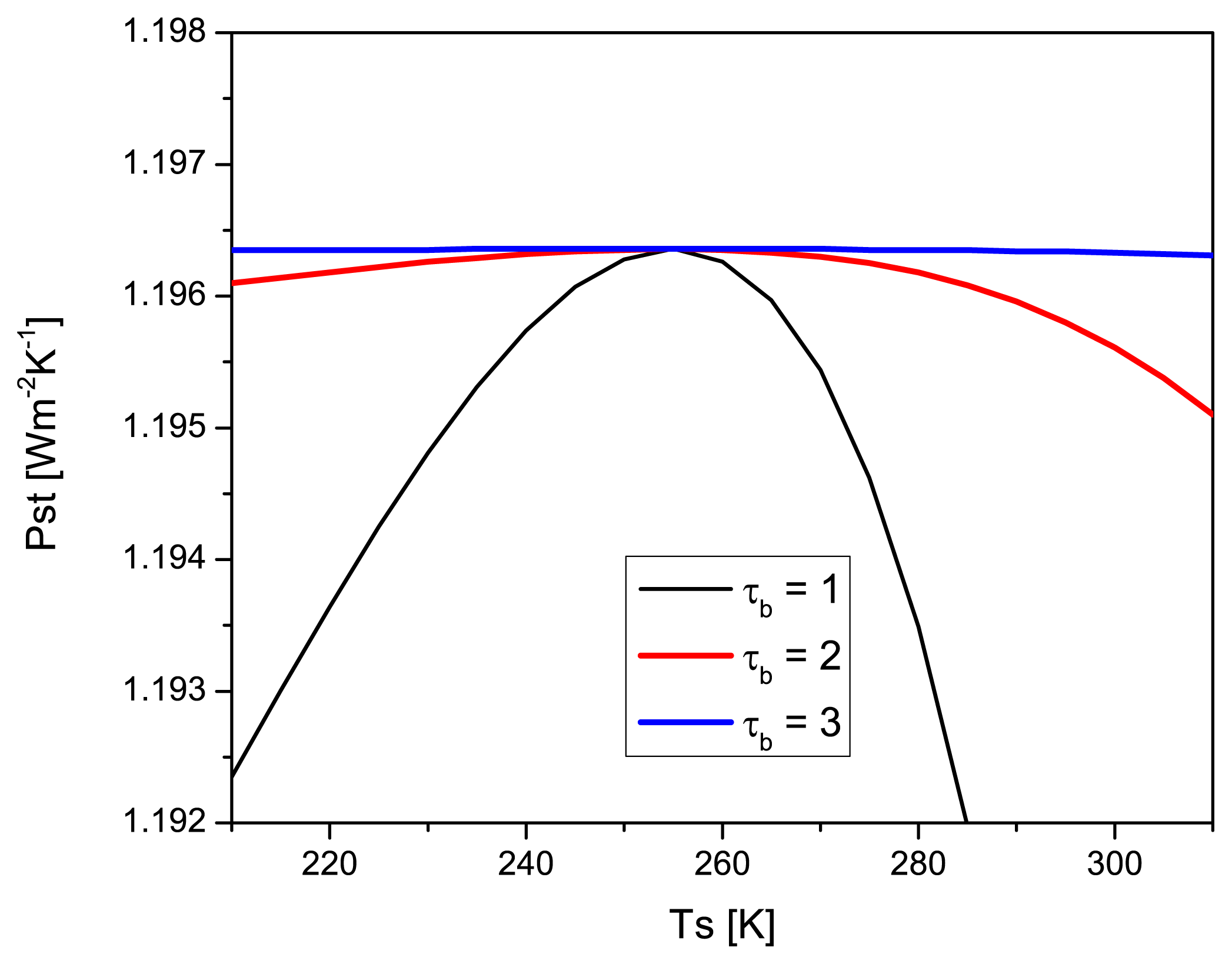
It is seen that it does not depend on τ̃b. Figure 4 shows this rate for three different greenhouse gas amounts (increasing with optical depth τb). The maxima coincide at the effective temperature Tef, i.e., when there is no temperature contrast between the upper and lower layers (cf. Equation (4)). A uniformly warm planet at its effective temperature maximizes its global entropy production rate, with the highest rate being given by (η+(τb) = 0 for Ta = Ts, cf. [9])
For a sufficiently opaque atmosphere in the infrared (τb ≳ 3), the rates for any temperature difference are nearly equal to the maximum rate, so we may conclude that a planet like Earth or Venus produces total entropy at nearly the maximum rate possible. Actually, both planets produce still more entropy, as we have not included the production rate due to scattering of the sun’s radiation, the calculation of which is rather thorny, involving as it does such a complex process as polarization [24]. The energy scattered back into space has been subtracted from the incoming amount in the formulation of the constraint (4), so the planet’s postulated manifold steady states are energetically comparable.
The rates in Figures 3 and 4 make it plain that by taking into account the entropy production due to radiative exchange of energy, there is no risk of violating the second law, even with an idealized model as ours which exhibits, outside the “Clausius-Duhem interval”, steady negative entropy production rates from undisclosed material processes.
5. Conclusions
The results presented above graphically lend themselves to discussion from different perspectives. In any event, the exercise is apt to teach us some noteworthy lessons.
By confining myself to the model’s abstract thermodynamics I wish to draw explicitly but three partly alternate conclusions:
- (1)
The model as defined is inadmissible and even impossible to realize, because for some (most) eligible surface temperatures Ts it would have to be attended by negative material entropy production rates. These, while they do not violate the second law, do violate the Clausius-Duhem inequality. Readers wishing to cling to the inequality as a universal restriction on constitutive equations have no choice but to reject the model’s thermal structure as unfeasible either in nature or the laboratory. They then could point to the Clausius-Duhem inequality for saving them the effort to find or create such a system.
- (2)
The model’s peculiar thermal structure is admissible to the extent that it satisfies the Clausius-Duhem inequality, which is the case for an interval of surface temperatures that are close to the temperature at which the model exhibits the maximum stationary material entropy production rate. For some values of optical depths, the temperature interval may vanish, and the resulting temperature uniformity leads to a vanishing material entropy production rate.
- (3)
If by one means or another the model could be realized, within the range of arbitrary temperature differences Ts−Ta permitted by the energy constraint, or at least be accepted as a valid idealization of a natural or laboratory system, qualms regarding the violation of the Clausius-Duhem inequality can be serenely set aside, for the latter would not be an effective constraint to constitutive equations. The model in fact does not violate the second law of thermodynamics.
The second conclusion I should like to interpret in different terms. The model presented enabled us to calculate explicitly both the term involving the radiative entropy supply in the Clausius-Duhem inequality and the total entropy production rates in the more general entropy inequality. Calculated figures proved the former inequality to be inconsistent with some steady-state temperature configurations. If we are to espouse the Clausius-Duhem inequality as the expression of the second law of thermodynamics for general continua, we cannot but dismiss the model for temperatures that are (indirectly) associated with negative material production rates Pm, which was shown to be the case if these are not close to the maximum rate. For certain parameter values this highest rate is only realized by thermal uniformity, Ta = Ts = Tef, and only radiative processes could then be held responsible for maintaining that steady state, without the aid of any (irreversible) material processes. But note that a uniform temperature is generally not the rigorous solution of the semi-gray radiation problem [25].
This interpretation is not compelling, however. Neither the Clausius-Duhem inequality nor the principle of maximum entropy production are universally acclaimed as being beyond controversy. Of those who object to the “MEP” principle, I cite only the recent paper [26], in which the authors need not appeal to arguments beyond the phenomenological theory of the present essay. And while the Clausius-Duhem inequality is indeed looked upon by many as the continuum-mechanical expression of the second law, occasionally doubts have been, and continue to be, raised concerning its construction. Müller [27] states that there are “awkward points about rational thermodynamics, the most obvious one being that, for the exploitation of the Clausius-Duhem inequality, it needs arbitrarily adjustable supplies ... r(x, t) in the field equations”. Müller’s shifting view on this issue may be judged against the footnote on p. 165 of his earlier grand book [29], where he explicitly rejected objections of this kind. Our model shows that indeed r can be adjusted, at least to some extent, so his objection is not as severe as it might seem at first. Málek & Rajagopal [28] express concern about the practice of eliminating r in the process of deriving constitutive equations, because then “one cannot take into account the different responses which materials have with respect to radiant heating”. They note that the use of the Clausius-Duhem inequality “to obtain restrictions would lead to the undesirable result that the radiant heating ought to be exactly that which leads to the balance of energy”. This is certainly a valid stricture. We have taken a slightly different stance, for we postulate unknown energy sources so as to keep up a presumed thermal uniformity in both layers, our sole wish having been to ascertain whether such a particular temperature distribution obeys the Clausius-Duhem inequality. Faced with the fact that the latter is not borne out for some parameter values of the model, we nonetheless need not dismiss it altogether as inadmissible or impossible, for we were able to see, by reviewing older work that duly allowed us to take into account the radiative contribution to the entropy production rate, that the second law of thermodynamics is never at stake.
Leaning as we do toward the third conclusion, we close this essay by intimating that whenever radiation has an import for thermomechanical material processes, the irreversible character of the radiative heating and cooling ought to be accounted for in an expression of the second law of thermodynamics. The incorporation of radiation into the latter we have shown to be in conformity with the entropy inequality of recently generalized continuum thermodynamics.
On the other hand, the maximum entropy principle, if effective, would militate in favor of the widespread disregard of the thermodynamics of the radiation field, which is viewed merely as an external source of energy in applications of the second law of thermodynamics to a continuum.
List of Some Symbols
| F̃↓(τ̃) | downward shortwave energy flux density (from hot exterior source) at shortwave optical depth τ̃ corresponding to height z |
| F̃↓(0) | incident flux density at the top of atmosphere (where density of absorbing matter is negligible) (= Q0μ⊚) |
| F↓(τ) | downward longwave energy flux density (from atmosphere) at infrared optical depth τ corresponding to height z |
| F↑(τ) | upward longwave energy flux density (from surface and atmosphere) at infrared optical depth τ corresponding to height z |
| F↑(0) | outgoing longwave radiation (at the outer boundary of atmosphere) where density of emitting matter is negligible) |
| F | = F↓−F↑, net radiative energy flux density (gain) |
downward shortwave entropy flux density (from hot exterior source) at top of the atmosphere | |
outgoing infrared entropy flux density at top of atmosphere | |
| Φ* | , net radiative entropy flux density (gain) |
monochr. energy radiance at depth τ and for μ > 0 | |
monochr. energy radiance at depth τ and for μ < 0 | |
monochr. entropy radiance at depth τ and for μ > 0 | |
monochr. entropy radiance at depth τ and for μ < 0 | |
| μ⊚ | = cos θ⊚, θ⊚ zenith angle of average position of sun |
| Pm | entropy production rate of the model (per unit of area except in Equation (3)) due to irreversible processes in matter |
| Pr | entropy production rate of the model (per unit of area) due to irreversible interaction of radiation with matter |
| Pst | total steady-state entropy production of the model (Pst = Pm +Pr) |
| Q0 | = F̃↓(0)/μ⊚ = 1367 Wm−2, solar constant of the model |
| r | energy supply rate to matter due to radiative interaction |
| r± | same as r but restricted to electromagnetic waves traveling inward (−) or outwardly (+) of the model layers |
| r̃ | same as r but referring only to solar (shortwave) radiation |
| ra, rs | same as r, with subindices a and s denoting rates in the atmosphere and surface, respectively |
| Ta | temperature of upper layer (atmosphere) |
| Ts | temperature of lower layer (surface) |
| Tef | effective temperature (overall thermal level of the planet) |
| T⊚ | temperature of exterior source (sun) |
entropy sources associated with entropy radiances of rays for which | |
| ς | optical depth of surface layer, , h = Hb+z |
| τ | infrared optical depth ( ), z altitude above z = 0 |
| τ̃ | shortwave optical depth ( ) |
| θ(μ) | zenith angle of a ray, cf. Figure 1; μ ≡ cos θ |
| ε, εs | ε = τ̃/τ, εs = σ̃/ς |
Acknowledgments
The author thanks Thomas Frisius for constant spurring to carry on with this topic, and also to Robert Niven for prevailing on me to contribute to his special issue on MEP in spite of very adverse circumstances. Finally, I should be liable to the charge of ingratitude, should I fail to mention my debt to the German Science Foundation (DFG) for its support of the Cluster of Excellence 177 Climate System Analysis and Prediction (CliSAP), where this work was brought to fruition.
Conflicts of Interest
The author declares there are no conflicts of interest.
References
- Truesdell, C.A.; Toupin, R.A. The Classical Field Theories. In Encyclopedia of Physics; Flügge, S., Ed.; Springer-Verlag: Berlin, Germany, 1960; Volume III/1, pp. 226–793. [Google Scholar]
- Coleman, B.; Noll, W. The thermodynamics of elastic materials with heat conduction and viscosity. Arch. Rational Mech. Anal 1963, 13, 167–178. [Google Scholar]
- Paltridge, G.W. Stumbling into the MEP racket: An historical perspective. In Non-equilibrium Thermodynamics and the Production of Entropy; Kleidon, A., Lorenz, R.D., Eds.; Springer-Verlag: Berlin, Germany, 2005. [Google Scholar]
- Dyke, J.; Kleidon, A. The maximum entropy production prnciple: Its theoretical foundations and applications to the Earth system. Entropy 2010, 12, 613–630. [Google Scholar]
- Liu, I-S. Continuum Mechanics; Springer-Verlag: Berlin, Germany, 2002. [Google Scholar]
- Gurtin, M.E.; Fried, E.; Anand, L. The Mechanics and Thermodynamics of Continua; Cambridge University Press: Cambridge, UK, 2010. [Google Scholar]
- Astarita, G.; Marrucci, G. Principles of Non-Newtonian Fluid Mechanics; McGraw-Hill: London, UK, 1974. [Google Scholar]
- Hutter, K.; Jöhnk, K. Continuum Methods of Physical Modeling; Springer-Verlag: Berlin, Germany, 2004. [Google Scholar]
- Pelkowski, J. On entropy production by radiative processes in a conceptual climate model. Meteorol. Z 2012, 21, 439–457. [Google Scholar]
- Goody, R.M.; Yung, Y.L. Atmospheric Radiation. Theoretical Basis; Oxford University Press: New York, NY, USA, 1989. [Google Scholar]
- Chandrasekhar, S. Radiative Transfer; Clarendon Press: Oxford, UK, 1950. [Google Scholar]
- Foukal, P. Solar Astrophysics; John Wiley & Sons, Inc: New York, NY, USA, 1990. [Google Scholar]
- Planck, M. Theorie der Wärmestrahlung; J.A. Barth: Leipzig, Germany, 1906. [Google Scholar]
- Callies, U.; Herbert, F. Radiative processes and nonequilibrium thermodynamics. J. Appl. Math. Phys 1988, 39, 242–266. [Google Scholar]
- Wildt, R. Radiative transfer and thermodynamics. Astrophys. J 1956, 123, 107–116. [Google Scholar]
- Pelkowski, J. Towards an accurate estimate of the entropy production due to radiative processes: Results with a gray atmosphere model. Meteorol. Atmos. Phys 1994, 53, 1–17. [Google Scholar]
- Feistel, R. Entropy flux and entropy production of stationary black-body radiation. J. Non-Equilib. Thermodyn 2011, 36, 131–139. [Google Scholar]
- Schatzman, E. Les plasmas en astrophysique. La théorie des gaz neutres et ionisés École d’été de physique théorique, Les Houches (tiré à part: Hermann, Paris). 1959. (In French). [Google Scholar]
- Essex, C. Radiation and the irreversible thermodynamics of climate. J. Atmos. Sci 1984, 41, 1985–1991. [Google Scholar]
- Pelkowski, J. Entropy production in a radiating layer near equilibrium: Assaying its variational properties. J. Non-Equilib. Thermodyn 1997, 22, 48–73. [Google Scholar]
- Weiss, W. The balance of entropy on earth. Cont. Mech. Thermodyn 1996, 8, 37–51. [Google Scholar]
- Müller, I.; Ruggeri, T. Rational Extended Thermodynamics, 2nd ed; Springer Tracts in Natural Philosophy; Springer-Verlag: New York, NY, USA, 1998; Volume 37. [Google Scholar]
- Wilmanski, K. Continuum Thermodynamics, Part I, Foundations; World Scientific Publishing Co: Singapore, 2008. [Google Scholar]
- Callies, U. Entropy production by atmospheric scattering of light. Beitr. Phys. Atmos 1989, 62, 212–226. [Google Scholar]
- Pelkowski, J.; Chevallier, L.; Rutily, B.; Titaud, O. Exact results in modeling planetary atmospheres—III. The general theory applied to the Earth’s semi-gray atmosphere. J. Quant. Spectrosc. Rad. Transfer 2008, 109, 43–51. [Google Scholar]
- Nicolis, C.; Nicolis, G. Stability, complexity and the maximum dissipation conjecture. Q. J. R. Meteorol. Soc 2010, 136, 1161–1169. [Google Scholar]
- Müller, I. Entropy in Nonequilibrium. In Entropy; Greven, A., Keller, G., Warnecke, G., Eds.; Princeton University Press: Princeton, NJ, USA, 2003; Volume Chapter 5. [Google Scholar]
- Málek, J.; Rajagopal, K.R. Mathematical Properties of the Solutions to the Equations Governing the Flow of Fluids with Pressure and Shear Rate Dependent Viscosities. In Handbook of Mathematical Fluid Dynamics; Elsevier: Amsterdam, The Netherlands, 2007; Volume 4, Chapter 7. [Google Scholar]
- Müller, I. Thermodynamics; Pitman: London, UK, 1985. [Google Scholar]


© 2014 by the authors; licensee MDPI, Basel, Switzerland This article is an open access article distributed under the terms and conditions of the Creative Commons Attribution license (http://creativecommons.org/licenses/by/3.0/).
Share and Cite
Pelkowski, J. On the Clausius-Duhem Inequality and Maximum Entropy Production in a Simple Radiating System. Entropy 2014, 16, 2291-2308. https://doi.org/10.3390/e16042291
Pelkowski J. On the Clausius-Duhem Inequality and Maximum Entropy Production in a Simple Radiating System. Entropy. 2014; 16(4):2291-2308. https://doi.org/10.3390/e16042291
Chicago/Turabian StylePelkowski, Joachim. 2014. "On the Clausius-Duhem Inequality and Maximum Entropy Production in a Simple Radiating System" Entropy 16, no. 4: 2291-2308. https://doi.org/10.3390/e16042291