Computational Information Geometry in Statistics: Theory and Practice

Abstract

A broad view of the nature and potential of computational information geometry in statistics is offered. This new area suitably extends the manifold-based approach of classical information geometry to a simplicial setting, in order to obtain an operational universal model space. Additional underlying theory and illustrative real examples are presented. In the infinite-dimensional case, challenges inherent in this ambitious overall agenda are highlighted and promising new methodologies indicated.

1. Introduction

The application of geometry to statistical theory and practice has seen a number of different approaches developed. One of the most important can be defined as starting with Efron’s seminal paper [1] on statistical curvature and subsequent landmark references, including the book by Kass and Vos [2]. This approach, a major part of which has been called information geometry, continues today, a primary focus being invariant higher-order asymptotic expansions obtained through the use of differential geometry. A somewhat representative example of the type of result it generates is taken from [2], where the notation is defined:

Example 1 The bias correction of a first-order efficient estimator, $\widehat{\beta }$, is defined by:

$$b^a(\beta )=-\frac{1}{2n}{g}^{a{a}^{\prime }}\left\{g^{bc}{\Gamma }_{a^{\prime }bc}^{(-1)}+g^{\kappa \mathrm{\lambda }}{h}_{\kappa \mathrm{\lambda }{a}^{\prime }}^{(-1)}\right\},$$

and has the property that if$\widehat{\beta }*:=\widehat{\beta }-b(\beta )$ then:

$$E_{\beta }(\widehat{\beta }*-\beta )=O(n^{-3/2}).$$

The strengths usually claimed of such a result are that, for a worker fluent in the language of information geometry, it is explicit, insightful as to the underlying structure and of clear utility in statistical practice. We agree entirely However, the overwhelming evidence of the literature is that, while the benefits of such inferential improvements are widely acknowledged in principle, in practice, the overhead of first becoming fluent in information geometry prevents their routine use. As a result, a great number of powerful results of practical importance lay severely underused, locked away behind notational and conceptual bars.

This paper proposes that this problem can be addressed computationally by the development of what we call computational information geometry. This gives a mathematical and numerical computational framework in which the results of information geometry can be encoded as “black-box” numerical algorithms, allowing direct access to their power. Essentially, this works by exploiting the structural properties of information geometry, which are such that all formulae can be expressed in terms of four fundamental building blocks: defined and detailed in Amari [3], these are the +1 and −1 geometries, the way that these are connected via the Fisher information and the foundational duality theorem. Additionally, computational information geometry enables a range of methodologies and insights impossible without it; notably, those deriving from the operational, universal model space, which it affords; see, for example, [4–6].

The paper is structured as follows. Section 2 looks at the case of distributions on a finite number of categories where the extended multinomial family provides an exhaustive model underlying the corresponding information geometry. Since the aim is to produce a computational theory, a finite representation is the ultimate aim, making the results of this section of central importance. The paper also emphasises how the simplicial structures introduced here are foundational to a theory of computational information geometry. Being intrinsically constructive, a simplicial approach is useful both theoretically and computationally. Section 3 looks at how simplicial structures, defined for finite dimensions, can be extended to the infinite dimensional case.

2. Finite Discrete Case

2.1. Introduction

This section shows how the results of classical information geometry can be applied in a purely computational way. We emphasise that the framework developed here can be implemented in a purely algorithmic way, allowing direct access to a powerful information geometric theory of practical importance.

The key tool, as explained in [4], is the simplex:

$${\mathrm{\Delta }}^k:=\left\{\mathrm{\pi }={\left({\mathrm{\pi }}_0,{\mathrm{\pi }}_1,\dots ,{\mathrm{\pi }}_{\mathrm{k}}\right)}^{\top }:{\mathrm{\pi }}_{\mathrm{i}}\ge 0,{\displaystyle \sum _{\text{i}=0}^{\mathrm{k}}{\mathrm{\pi }}_{\mathrm{i}}=1}\right\},$$

(1)

with a label associated with each vertex. Here, k is chosen to be sufficiently large, so that any statistical model—by which we mean a sample space, a set of probability distributions and selected inference problem—can be embedded. The embedding is done in such a way that all the building blocks of information geometry (i.e., manifold, affine connections and metric tensor) can be numerically computed explicitly. Within such a simplex, we can embed a large class of regular exponential families; see [6] for details. This class includes exponential family random graph models, logistic regression, log-linear and other models for categorical data analysis. Furthermore, the multinomial family on k + 1 categories is naturally identified with the relative interior of this space, int(∆^k), while the extended family, Equation (1), is a union of distributions with different support sets.

This paper builds on the theory of information geometry following that introduced by [3] via the affine space construction introduced by [7] and extended by [8]. Since this paper concentrates on categorical random variables, the following definitions are appropriate. Consider a finite set of disjoint categories or bins $ℬ$ = {B_i}_iϵA. Any distribution over this finite set of categories is defined by a set, {π_i}_iϵa, which defines the corresponding probabilities. With “mix” connoting mixtures of distributions, we have:

Definition 1 The −1-affine space structure over distributions on $ℬ$ :={B_i}_i∈A is (X_mix, V_mix, +) where:

$$X_{mix}=\left\{{\left\{x_i\right\}}_{i\in A}|{\displaystyle \sum _{{}_{i\in A}}{x}_i=1}\right\},V_{mix}=\left\{{\left\{{\upsilon }_i\right\}}_{i\in A}|{\displaystyle \sum _{{}_{i\in A}}{\upsilon }_i=0}\right\}$$

and the addition operator, +, is the usual addition of sequences.

In Definition 1, the space of (discretised) distributions is a −1-convex subspace of the affine space, (X_mix, V_mix, +). A similar affine structure for the +1-geometry, once the support has been fixed, can be derived from the definitions in [7].

2.2. Examples

Examples 2 and 3 are used for illustration. The second of these is a moderately high dimensional family, where the way that the boundaries of the simplex are attached to the model is of great importance for the behaviour of the likelihood and of the maximum likelihood estimate. In general, working in a simplex, boundary effects mean that standard first order asymptotic results can fail, while the much more flexible higher order methods can be very effective. The other example is a continuous curved exponential family, where both higher order asymptotic sampling theory results and geometrically-based dimension reduction are described.

Example 2 The paper [9] models survival times for leukaemia patients. These times, recorded in days, start at the time of diagnosis, and there are 43 observations; see [10] for details. We further assume that the data is censored at a fixed value. It was observed that a censored exponential distribution gives a reasonable, but not exact, fit. As discussed in [11], this gives a one-dimensional curved exponential family inside a two-dimensional regular exponential family of the form:

$$\text{exp }\left[{\lambda }_{1}x+{\lambda }_{2}y-\log \left\{\frac{1}{{\lambda }_2}(e^{{\lambda }_{2}t}-1)+e^{{\lambda }_1+{\lambda }_{2}t}\right\}\right],$$

(2)

where y = min(z, t) and x = I(z ≥ t), and the embedding map is given by (λ₁(θ), λ₂₁θ)) = (−log θ, −θ).

As shown in [4], the loss due to discretisation can be made arbitrarily small for all information geometry objects. Thus, for example, using this computational approach, it is straightforward to compute the bias correction described in Example 1. Each of the terms in the asymptotic bias, i.e., the metric, g_ij, its inverse, g^ij, the Christoffel symbols, ${\Gamma }_{ijk}^{(-1)}$, and curvature term, h⁽⁻¹⁾, can be directly numerically coded as appropriate finite difference approximations to derivatives. Thus, “black-box” code can directly calculate the numerical value of the asymptotic bias, and this numerical value can then be used by those who are not familiar with information geometry. For example this calculation establishes the fact that, with this particular data set, the sample size is such that the bias is inferentially unimportant.

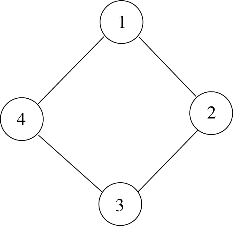
Example 3 The paper [12] discusses an undirected graphical model based on the cyclic graph of order four, shown in Figure 1, with binary random variables at each node. Without any constraints, there are 16 possible values for the graph, so model space can be thought of as a 15-dimensional simplex, including the relative boundary. However, the conditional independence relations encoded by the graph impose linear constraints in the natural parameters of the exponential family. Thus, the resultant model is a lower dimensional full exponential family and its closure.

As described in [12], the four cycle model is a seven dimensional exponential family, which is a +1-affine subspace of the +1-affine structure of the 15-dimensional simplex. The model can be written in the form:

$${\left(\frac{{\pi }_i\exp \left\{{\displaystyle {\sum }_{h=1}^8{\eta }_h{\upsilon }_{hi}}\right\}}{{\displaystyle {\sum }_{j=0}^{15}{\pi }_j\exp \left\{{\displaystyle {\sum }_{h=1}^8{\eta }_h{\upsilon }_{hj}}\right\}}}\right)}_{i=0}^{15}$$

(3)

for a given set of linearly independent vectors${\left\{{\upsilon }_h\right\}}_{h=1}^8$. The existence of the maximum likelihood estimate for η = (η_h) will depend on how the limit points of Model (3) meet the observed face of ∆¹⁵; that is, the span of the vertices (bins) having positive counts. Thus, a key computational task is to learn how a full exponential family, defined by a representation of the form of (3), is attached to boundary sub-simplices of the high-dimensional embedding simplex.

In order to visualise the geometric aspects of this problem, consider a lower dimensional version. Define a two-dimensional full exponential family by the vectors υ₁ = (1, 2, 3,4), υ₂ = (1, 4, 9, −1) and the uniform distribution base point, π_i, embedded in the three-dimensional simplex. The two-dimensional family is defined by the +1-affine space through (0.25, 0.25, 0.25, 0.25) spanned by the space of vectors of the form:

$$\alpha (1,2,3,4)+\beta (1,4,9,-1)=(\alpha +\beta ,2\alpha +4\beta ,3\alpha +9\beta ,4\alpha -\beta ).$$

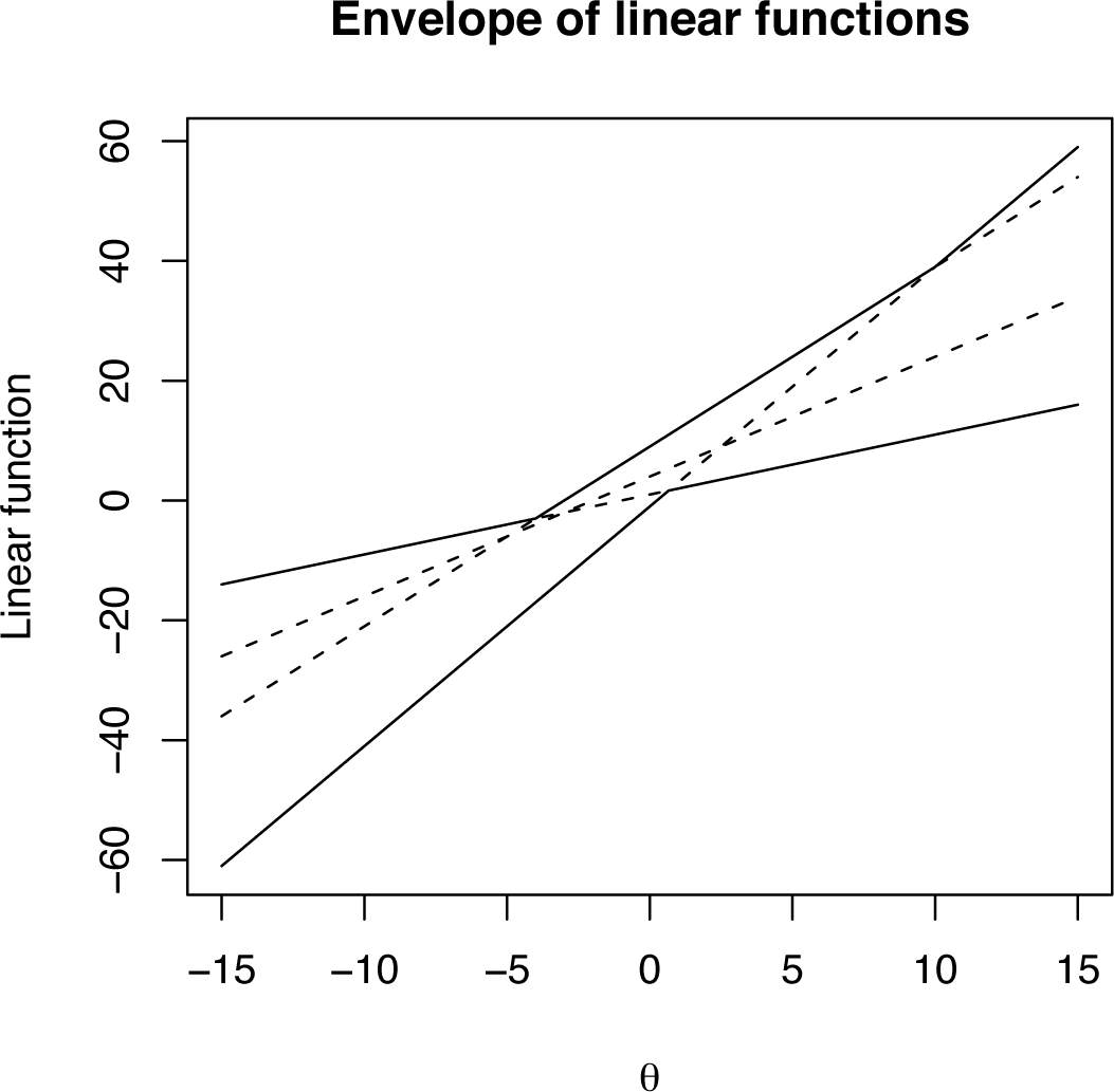
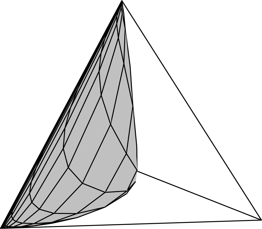
Consider directions from the origin obtained by writing α = θβ, giving, for each θ, a one-dimensional, full exponential family parameterized by β in the direction β(θ + 1, 2θ + 4, 3θ + 9, 4θ − 1). The aspect of this vector, which determines the connection to the boundary, is the rank order of its elements. For example, suppose the first component was the maximum and the last the minimum. Then, as β → ±∞, this one-dimensional family will be connected to the first and fourth vertex of the embedding four simplex, respectively. Note that changing the value of θ changes the rank structure, as illustrated in Figure 2. This plot shows the four element-wise linear functions of θ (dashed lines) and the salient overall feature of their rank order; that is, their upper and lower envelopes (solid lines). From this analysis of the envelopes of a set of linear functions, it can be seen that the function 2θ + 4 is redundant. The consequence of this is shown in Figure 3, which shows a direct computation of the two-dimensional family. It is clear that, indeed, only three of the four vertexes have been connected by the model.

In general, the problem of finding the limit points in full exponential families inside simplex models is a problem of finding redundant linear constraints. As shown in [13], this can be converted, via convex duality, into the problem of finding extremal points in a finite dimensional affine space. In the four-cycle model, this technique can construct all sub-simplices containing limit points of the four-cycle model. For example, it can be shown that all of the 16 vertices are part of the boundary. Once the boundary points have been identified as necessary and sufficient, conditions for the existence of the maximum likelihood in the +1-parameters can easily be found computationally [6].

2.3. Tensor Analysis and Numerical Stability

One of the most powerful set of results from classical information geometry is the way that geometrically-based tensor analysis is perfect for use in multi-dimensional higher order asymptotic analysis; see [14] or [15]. The tensorial formulation does, however, present a couple of problems in practice. For many, its very tight and efficient notational aspects can obscure rather than enlighten, while the resulting formulae tend to have a very large number of terms, making them rather cumbersome to work with explicitly. These are not problems at all for the computational approach described in this paper. Rather, the clarity of the tensorial approach is ideal for coding, where large numbers of additive terms, of course, are easy to deal with.

Two more fundamental issues, which the global geometric approach of this paper highlights, concern numerical stability. The ability to invert the Fisher information matrix is vital in most tensorial formulae, and so understanding its spectrum, discussed in Section 2.4, is vital. Secondly, numerical underflow and overflow near boundaries require careful analysis, and so, understanding the way that models are attached to the boundaries of the extended multinomial models is equally important. The four-cycle model, to which we now return, illustrates computational information geometry doing this effectively.

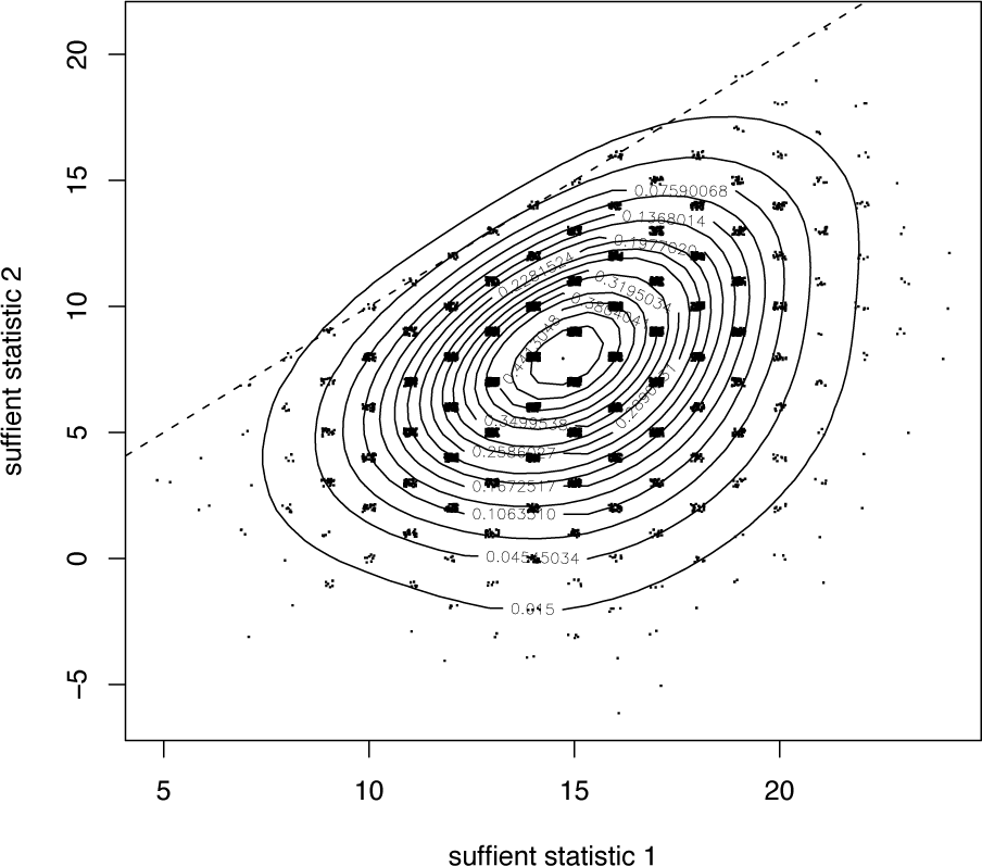
Example 4 The multivariate Edgeworth approximation to the sampling distribution of part of the sufficient statistic for the four-cycle model is shown in Figure 4. Using the techniques described above, a point near the boundary of the 15-simplex has been selected as the data generation process. For illustration, we focus on the marginal distribution of two components of the sufficient statistic, though any number could have been chosen. The boundary forces constraints on the range of the sufficient statistics, shown by the dashed line in the plot. The points, jittered for clarity, show the distribution computed by simulation. It is typical that such boundary constraints prevent standard first order methods from performing well, but the greater flexibility of higher order methods can be seen to work well here. As discussed above, methods, such as the multivariate Edgeworth expansion, can be strongly exploited in a computational framework, such as ours. Note, the discretization that can be observed in the figure is extensively discussed in [6].

2.4. Spectrum of Fisher Information

We focus now on the second numerical issue identified above. In any multinomial, the Fisher information matrix and its inverse are explicit. Indeed, the 0-geodesics and the corresponding geodesic distance are also explicit; see [2] or [3]. However, since the simplex glues together multinomial structures with different supports and the computational theory is in high dimensions, it is a fact that the Fisher information matrix can be arbitrarily close to being singular. It is therefore of central interest that the spectral decomposition of the Fisher information itself has a very nice structure, as shown below.

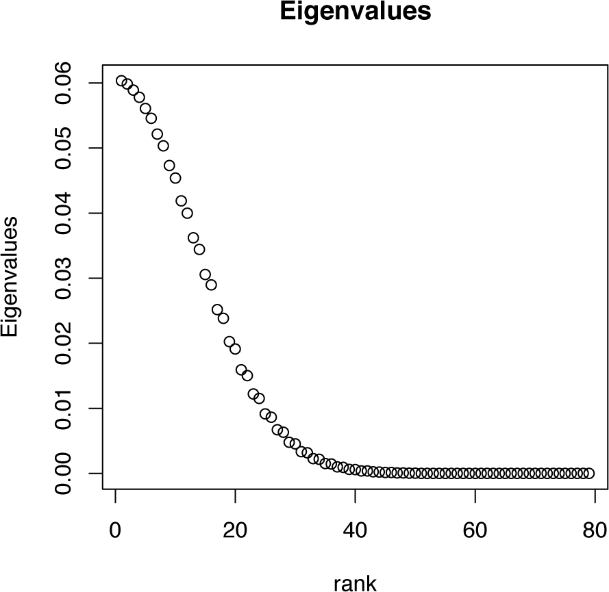
Example 5 Consider a multinomial distribution based on 81 equal width categories on [−5, 5], where the probability associated to a bin is proportional to that of the standard normal distribution for that bin. The Fisher information for this model is an 80 × 80 matrix, whose spectrum is shown in Figure 5. By inspection, it can be seen that there are exponentially small eigenvalues, so that while the matrix is positive definite, it is also arbitrarily close to being singular. Furthermore, it can be seen that the spectrum has the shape of a half-normal density function and that the eigenvalues seem to come in pairs. These facts are direct consequences of the general results below.

With π₋₀ denoting the vector of all bin probabilities, except π₀, we can write the Fisher information matrix (in the +1 form) as N times:

$$I(\pi ):=diag({\pi }_{-0})-{\pi }_{-0}{\pi }_{-0}^T.$$

This has an explicit spectral decomposition, which can be computed by using interlacing eigenvalue results (see for example [16], Chapter 4). In particular, if the diagonal matrices, diag(π₁, …, π_k) and $diag({\mathrm{\lambda }}_1{I}_{m_1}|\dots |{\mathrm{\lambda }}_g{I}_{m_g})$, agree up to a row-and-column permutation, where g > 1 and λ₁ >…> λ_g > 0, then I(π) has ordered spectrum:

$${\mathrm{\lambda }}_1>{\tilde{\mathrm{\lambda }}}_1>\dots >{\mathrm{\lambda }}_g>{\tilde{\mathrm{\lambda }}}_g\ge 0,$$

(4)

with ${\tilde{\lambda }}_g>0\iff {\pi }_0>0$, each λ_i having multiplicity m_i – 1, while each ${\tilde{\lambda }}_g$ is simple.

We give a complete account of the spectral decomposition (SpD) of i(π). There are four cases to consider, the last having the generic spectrum of (4). Without loss, after permutation, assume now π₁ ≥…≥ π_k. The four cases are:

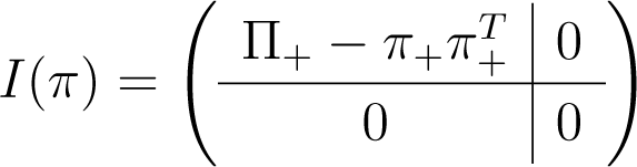
Case 1 For some l < k, the last k – l elements of π₋₀ vanish: the sub-case l = 0 ⇔ π₀ = 1 ⇔ i(π) = 0 is trivial. Otherwise, writing π₊ = (π₁,…, π_l)^t and Π₊ = diag(π₊), the SpD of:

follows at once from that of ${\Pi }_{+}-{\mathrm{\pi }}_{+}{\mathrm{\pi }}_{+}^T$, given below.

Case 2 k = 1: this case is trivial.

Case 3 k > 1, π = λ1_k, λ > 0: the SpD of I(π) is:

$$\mathrm{\lambda }{C}_k+\mathrm{\lambda }(1-k\mathrm{\lambda })J_k$$

where C_k = I_k – J_k and $J_k=k^{-1}{1}_k{1}_k^T$. Here, λ has multiplicity k – 1 and eigenspace [Span(1_k)]^⊥, while $\tilde{\lambda }:=\lambda (1-k\lambda )$ has multiplicity one and eigenspace Span(1_k). In particular, since 1 – π₀ = kλ, it follows that:

$$I(\mathrm{\pi })\text{ is singular}\iff {\mathrm{\pi }}_0=0.$$

Case 4 ${\mathrm{\pi }}_{-0}={\left({\mathrm{\lambda }}_1{1}_{m_1}^T|\dots |{\mathrm{\lambda }}_g{1}_{m_g}^T\right)}^T$, g > 1 and λ₁ >…> λ_g > 0:

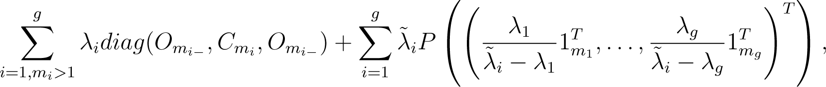
This is the generic case, having the spectrum of (4) above. Denoting by O_m the zero matrix of order m × m and by P(ν) the rank one orthogonal projector onto Span(ν), (ν ≠ 0), the SpD is:

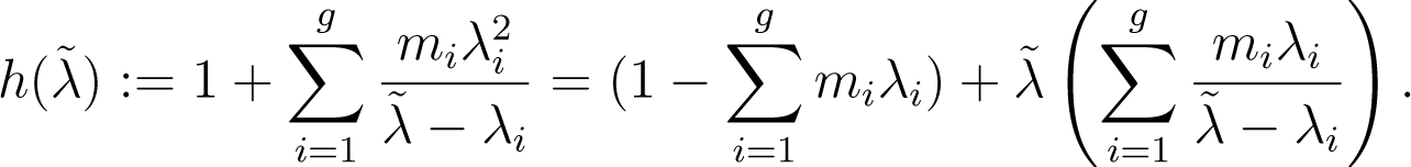
where: m_i− = ∑{m_j|j < i}, m_i+ = ∑{m_j|j > i} and the ${\tilde{\lambda }}_i$ are the zeros of:

In particular, $\{{\tilde{\lambda }}_i:i=1,\dots ,g\}$ are simple eigenvalues satisfying (4) while, whenever m_i > 1, λ_i, is also an eigenvalue having multiplicity m_i – 1. Further, expanding det(I(π)), we again find:

$$I(\mathrm{\pi })\text{ is singular}\iff {\mathrm{\pi }}_0=0,$$

so that ${\tilde{\lambda }}_g>0\iff {\pi }_0>0$, as claimed. Finally, we note that each ${\tilde{\lambda }}_i(i<g)$ is typically (much) closer to λ_i than to λ_i+1. For, considering the graph of x → 1/x, h ((λ_i + λ_i+1)/2 + δ(λ_i – λ_i+1)/2) (−1 < δ < +1) is well-approximated by:

$$1-\frac{2m_i{\mathrm{\lambda }}_i^2}{{\text{(λ}}_i-{\mathrm{\lambda }}_{i+1})(1-\delta )}+\frac{2m_{i+1}{\mathrm{\lambda }}_{i+1}^2}{{\text{(λ}}_i-{\mathrm{\lambda }}_{i+1})(1+\delta )}$$

whose unique zero δ_∗ over (−1, 1) is positive whenever, as will typically be the case, m_i = m_i+1 (both will usually be one), while (m_iλ_i + m_i+1λ_i+1) < 1/2. Indeed, a straightforward analysis shows that, for any mi and m_i+1, δ_∗ = 1 + O(λ_i) as λ_i → 0.

2.5. Total Positivity and Local Mixing

Mixture modelling is an exemplar of a major area of statistics in which computational information geometry enables distinctive methodological progress. The −1-convex hull of an exponential family is of great interest, mixture models being widely used in many areas of statistical science. In particular, they are explored further in [5]. Here, we simply state the main result, a simple consequence of the total positivity of exponential families [17], that, generically, convex hulls are of maximal dimension. In this result, “generic” means that the +1 tangent vector, which defines the exponential family as having components that are all distinct.

Theorem 1 The −1-convex hull of an open subset of a generic one-dimensional exponential family is of full dimension.

Proof 1 For any (π_i) ∈ ∆^k with each π_i > 0, θ₀ < … < θ_k and s₀ < … < s_k, let B = (π(θ₀),…, π(θ_k)) have general element:

$${\pi }_i({\theta }_j):={\pi }_i\exp [s_i{\theta }_j-\psi ({\theta }_j)].$$

Further, let$\tilde{B}=B-\pi ({\theta }_0)1_{k+1}^T$, whose general column is π(θ_j) – π(θ₀). Then, it suffices to show that$\tilde{B}$ has rank k. However, using [18] (p. 33), $Rank(\tilde{B})=Rank(B)-1$, so that:

$$Rank(\tilde{B})=k\iff B is nonsingular\iff B^{*}isnonsingular,$$

where B* = (exp[s_iθ_j]). It suffices, then, to recall [17] that K(x, y) = exp(xy) is strictly total positive (of order ∞), so that det B* > 0.

3. Infinite Dimensional Structure

This section will start to explore the question of whether the simplex structure, which describes the finite dimensional space of distributions, can extend to the infinite dimensional case. We examine some of the differences with the finite dimensional case, illustrating them with clear, commonly occurring examples.

3.1. Infinite Dimensional Information Geometry: A Review

In the previous sections, the underlying computational space is always finite dimensional. This section looks at issues related to an infinite dimensional extension of the theory in that paper. There is a great deal of literature concerning infinite dimensional statistical models. The discussion here concentrates on information geometric, parametrisation and boundary issues.

The information geometry theory of Amari [3] has a geometric foundation, where statistical models (typically full and curved exponential families) have a finite dimensional manifold structure. When considering the extension to infinite dimensional cases, Amari notes the problem of finding an “adequate topology” [3] (p. 93). There has to be very interesting work following up this topological challenge. By concentrating on distributions with a common support, the paper [19] uses the geometry of a Banach manifold, where local patches on the manifold are modelled by Banach spaces, via the concept of an Orlicz space. This gives a structure that is analogous to an infinite dimensional exponential family, with mean and natural parameters and including the ability to define mixed parametrisations. One drawback of this Banach structure, as pointed out in [20], is that the likelihood function with finite samples is not continuous on the manifold. Fukumizu uses a reproducing kernel Hilbert space structure rather than a Banach manifold, which is a stronger topology. There are strong connections between the approach taken in [20] and the material in Section 3.2, we note two issues here: (1) a focus on the finite nature of the data; and (2) using a Hilbert structure defined by a cumulant generating function. The approaches differ in that [20] uses a manifold approach rather than the simplicial complex as the fundamental geometric object. There is also other work that explicitly used infinite dimensional Hilbert spaces in statistics, a good reference being [21].

In this paper, in contrast to previous authors, a simplicial, rather than a manifold-based, approach is taken. This allows distributions with varying support, as well as closures of statistical families to be included in the geometry. Another difference in approach is the way in which geometric structures are induced by infinite dimensional affine spaces rather than by using an intrinsic geometry. This approach was introduced by [7] and extended by [8]. Spaces of distributions are convex subsets of the affine spaces, and their closure within the affine space is key to the geometry.

In exponential families, the −1-affine structure is often called the mean parametrisation, and using moments as parameters is one very important part of modelling. In the infinite dimensional case, the use of moments as a parameter system is related to the classical moment problem—when does there exist a (unique) distribution whose moments agree with a given sequence?—which has generated a vast literature in its own right; see [22–24]. In general terms, the existence of a solution to the moment problem is connected to positivity conditions on moment matrices. Such conditions have been used in connection to the infinite dimensional geometry of mixture models [25]. Uniqueness, however, is a much more subtle problem: sufficient conditions can be formulated in terms of the rate of growth of the moments [24]. Counter examples to general uniqueness results include the log-normal distribution [23].

The geometry of the Fisher information is also much more complex in general spaces of distributions than in exponential families. Simple mixture models, including two-component mixtures of exponential distributions [26], can have “infinite” expected Fisher information, which gives rise to non-standard inference issues. Similar results on infinitely small (and large) eigenvalues of covariance operators are also noted in [20]. Since the Fisher information is a covariance, the fact that it does not exist for certain distributions or that its spectrum can be unbounded above or arbitrarily close to zero is not a surprise. However, these observations do need to be taken into account when considering the information geometry of infinite dimensional spaces.

The rest of this section looks at the topology and geometry of the infinite dimensional simplex and gives some illustrative examples, which, in particular, show the need for specific Hilbert space structures, discussed in the final section.

3.2. Topology

For simplicity and concreteness, in this section, we will be looking at models for real valued random variables. In this paper, we restrict attention to the cases where the sample space is ℝ⁺ or ℝ and has been discretised to a countably infinite set of bins, B_i, with i ∈ ℕ or ℤ, respectively. In the finite case, the basic object is the standard simplex, ∆^k, with k + 1 bins. We generalise this to countable unions of such objects. Of these, one is of central importance, denoted by ∆_emp or simply ∆, because it is the smallest object that contains all possible empirical distributions.

Definition 2 For any finite subset of bins, indexed by $ℐ$ ⊂ ℕ or ℤ, denote

$${\mathrm{\Delta }}_I=\left\{\mathrm{x}={(x_i)}_{i\in I}:x_i\ge 0,{\displaystyle \sum _{i\in I}{x}_i=1}\right\}.$$

We take the union of all such sets ∪_|$ℐ$|<∞ Δ_$ℐ$, where |$ℐ$| denotes the number of elements of the index set. This can always be written as:

In what follows, it is important to note that for any given statistical inference problem, the sample size, n, is always finite, even if we frequently use asymptotic approximations, where n → ∞. Thus, the data, as represented by the empirical distribution, naturally lie in the space, ∆. However, many models, used in the given inference problem, will have support over all bins, so the models most naturally lie in the “boundary” constructed using the closures of the set. These objects are subsets of sequence spaces, and the corresponding topologies can be constructed from the Banach spaces, ℓ_p, p ∈ [1, ∞]. The following results follow directly from explicit calculations, where we note that in this section, since all terms are non-negative, convergence always means absolute convergence. In particular, arbitrary rearrangements of series do not affect the existence of limits or their values.

Example 6 Consider the sequence of “uniform distributions”${\mathrm{x}}^{(n)}=\left(\frac{1}{n},\dots ,\frac{1}{n},0,\dots \right)$ as elements of ∆. This has an ℓ_p limit of the zero sequence for p ∈ (1, ∞].

Proposition 1 The ℓ_p extreme points of ∆, for p ∈ (1, ∞], are the zero sequence and the sequences, δ_i (i ∈ ℤ), with one as the i – th element and zero elsewhere.

For p ∈ [1, ∞], let ${\overline{\mathrm{\Delta }}}_p\subset {\ell }_p$ denote the ℓ_p closure of ∆.

Theorem 2 (a)${\overline{\mathrm{\Delta }}}_1=\left\{\mathrm{x}={(x_i)}_{i\in \mathbb{Z}}:x_i\ge 0,{\displaystyle {\sum }_{i\in I}{x}_i=1}\right\}.$

(b)${\overline{\mathrm{\Delta }}}_{\infty }=\left\{\mathrm{x}={(x_i)}_{i\in \mathbb{Z}}:x_i\ge 0,{\displaystyle {\sum }_{i\in I}{x}_i\le 1}\right\}.$

(c) For$p\in (1,\infty ),{\overline{\mathrm{\Delta }}}_p={\overline{\mathrm{\Delta }}}_{\infty }=\left\{\mathrm{x}={(x_i)}_{i\in \mathbb{Z}}:x_i\ge 0,{\displaystyle {\sum }_{i\in I}{x}_i\le 1}\right\}.$

Proof 2 (a) It is immediate that$\left\{\mathrm{x}={(x_i)}_{i\in \mathbb{Z}}:x_i\ge 0,{\displaystyle {\sum }_{i\in \mathbb{Z}}{x}_i=1}\right\}\subseteq {\overline{\mathrm{\Delta }}}_1$. Conversely, if$\overline{x}$ is a limit point, then all its elements must be non-negative. Finally, if${\displaystyle {\sum }_{i=1}^{\infty }{\overline{x}}_i}$ is not bounded above by one, then there exists N, such that${\displaystyle {\sum }_{i=1}^N{\overline{x}}_i}>1+\in$ for some ∈ > 0. Hence, ${\displaystyle {\sum }_{i=1}^{\infty }|{\overline{x}}_i-x_i^{(n)}|}\ge {\displaystyle {\sum }_{i=1}^N|{\overline{x}}_i-x_i^{(n)}|}\ge {\displaystyle {\sum }_{i=1}^N{\overline{x}}_i-}{\displaystyle {\sum }_{i=1}^N{x}_i^{(n)}>\in }$ for all n, which contradicts convergence. If${\displaystyle {\sum }_{i=1}^{\infty }{\overline{x}}_i}<1-\in$, then${\displaystyle {\sum }_{i=1}^{\infty }|{\overline{x}}_i-x_i^{(n)}|}\ge {\displaystyle {\sum }_{i=1}^{\infty }{x}_i^{(n)}-}{\displaystyle {\sum }_{i=1}^{\infty }{\overline{x}}_i>\in }$, which again contradicts convergence.

(b) It is again immediate that$\{\mathrm{x}={(x_i)}_{i\in \mathbb{Z}}:x_i\ge 0,{\displaystyle {\sum }_{i\in \mathbb{Z}}{x}_i=1}\}\subseteq {\overline{\mathrm{\Delta }}}_{\infty }$. However, by Example 6, the zero sequence is also in${\overline{\mathrm{\Delta }}}_{\infty }$, so that$\{\mathrm{x}={(x_i)}_{i\in \mathbb{Z}}:x_i\ge 0,{\displaystyle {\sum }_{i\in \mathbb{Z}}{x}_i\le 1}\}\subseteq {\overline{\mathrm{\Delta }}}_{\infty }$.

Conversely, by contradiction, it is easy to see that all elements of the closure must have non-negative elements. Finally, for any$\overline{x}\in {\overline{\mathrm{\Delta }}}_{\infty }$, if${\displaystyle {\sum }_{i=1}^{\infty }{\overline{x}}_i}$ is not bounded above by one, there exists N, such that${\displaystyle {\sum }_{i=1}^N{\overline{x}}_i>1+\in }$ for some ∈ > 0. For any sequence of points, x⁽ⁿ⁾ in ∆, we have that${\displaystyle {\sum }_{i=1}^N{x}_i^{(n)}\le 1}$, so that, for i = 1, …, N, the maximum value of$|x_i^{(n)}-{\overline{x}}_i|>\in /N$. Hence, for all sequences, x⁽ⁿ⁾, we have${\Vert x^{(n)}-\overline{x}\Vert }_{\infty }>\in /N$, which contradicts$\overline{x}$ being in the closure.

(c) This follows essentially the same argument as (b) by noting in the case where${\displaystyle {\sum }_{i=1}^{\infty }{\overline{x}}_i}$ is not bounded above by one, we have:

$${\Vert x^{(n)}-\overline{x}\Vert }_p^p\ge {\displaystyle \sum _{i=1}^N|{\overline{x}}_i-x_i^{(n)}{|}^p\ge N\underset{i=1,\dots N}{{\displaystyle max}}|x_i^{(n)}-{\overline{x}}_i{|}^p>N^{1-p}{\in }^p}$$

for any sequences, x⁽ⁿ⁾, which contradicts x being in the closure.

It is immediate that the spaces, ∆ and ${\overline{\mathrm{\Delta }}}_1$, are convex subsets of ℓ₁ and that ${\overline{\mathrm{\Delta }}}_{\infty }$ is a convex set in ℓ_∞.

3.3. Geometry

In the same way as for the finite case, the −1-geometry can be defined using an affine space structure using the following definition.

Definition 3 Let $ℐ$ be a countable index set which is a subset of ℤ. The −1-affine space structure over distributions is (X_mix, V_mix, +), where:

$$X_{mix}=\{\text{x}=(x_i)|{\displaystyle \sum }_{ℐ}{x}_i=1,{\displaystyle \sum }_{ℐ}\left|x_i\right|<\infty ,\},V_{mix}=\{\text{v}={\upsilon }_i|{\displaystyle \sum }_{ℐ}{\upsilon }_i=0,{\displaystyle \sum }_{ℐ}|{\upsilon }_i|<\infty ,\},$$

and x + v = (x_i + v_i).

In order to define the +1-geometric structure, we also follow the approach used in the finite case. Initially, to understand the +1- structure, consider the case where all distributions have a common support, i.e., assume π_i > 0 for all i. We follow here the approach of [7].

Definition 4 Consider the set of non-negative measures on ℕ or ℤ and the equivalence relation defined by:

$$\left\{a_i\right\}\sim \left\{b_i\right\}\iff \exists \mathrm{\lambda }>0s.t.\forall i{a}_i=\mathrm{\lambda }{b}_i.$$

The equivalences classes of this are the points in the +1 geometry.

These points can be further partitioned into sets with the same support, i.e., supp(< a >) = {i:a_i > 0}, where this is clearly well-defined.

On sets of +1-points with the same support, we can define the +1-geometry in the same way as in the finite case. With “exp” connoting an exponential family distribution, we have:

Definition 5 For a given index set, $ℐ$, define X_exp to be all +1-points whose support equals $ℐ$, and define the vector space V_exp = {υ_i, i ∈ $ℐ$} with the operation, ⊕, defined by:

$$<x_i>\oplus {\upsilon }_i=\langle x_i\exp ({\upsilon }_i)\rangle ,$$

is an affine space. The +1-affine structure is then defined by (X_exp, V_exp, ⊕).

Theorem 3 If a and b lie in ∆ (or${\overline{\mathrm{\Delta }}}_1$) and have the same support, then$C(\rho )={\displaystyle \sum (a_i^{\rho }{b}_i^{(1-\rho )})<\infty }$ for ρ ∈ [0,1]. Hence, $\frac{a_i^{\rho }{b}_i^{(1-\rho )}}{C(\rho )}\in \mathrm{\Delta }(or{\overline{\mathrm{\Delta }}}_1)$.

Proof 3 Since a, b are absolutely convergent, the sequence, max(a_i, b_i), is also. Since we have:

$$0\le min(a_i,b_i)\le a_i^{\rho }{b}_i^{1-\rho }\le max(a_i,b_i)$$

it follows that C(ρ) < ∞, and we have the result.

This result shows that sets in ${\overline{\mathrm{\Delta }}}_1$ with the same support are +1-convex, just as the faces in the finite case are.

3.4. Examples

In order to get a sense of how the +1-geometry works, let us consider a few illustrative examples.

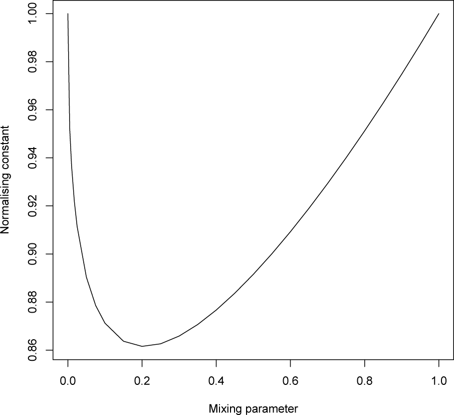
Example 7 If we denote the discretised standard normal density by a and the discretised Cauchy density by b and consider the path:

$$\frac{a_i^{\rho }{b}_i^{(1-\rho )}}{C(\rho )},$$

the normalising constant is shown in Figure 6. We see that at ρ = 0 (the Cauchy distribution), we have that the derivative of the normalising constant (i.e., the mean of the sufficient statistic) is tending to infinity. At the other end (ρ = 1), the model can be extended in the sense that the distribution exists for values greater than one.

Thus, in this example, the path joining the two distributions is an extended, rather than natural, exponential family, since we have to include the boundary point where the mean is unbounded.

Example 8 Let us return to Example 2, but now without the censoring. Thus, now, there is a countably infinite set of bins, and so, we can investigate its embedding in the infinite simplex. As discussed in [4], we shall discretise the continuous distribution by computing the probabilities associated to bins [c_i, c_i+1], i = 1, 2,….

For the exponential model, Exp(θ), the bin probabilities are simply:

$${\pi }_i(\theta )=\exp (-\theta c_i)-\exp (-\theta c_{i+1}).$$

Using this, the model will lie in the infinite simplex on the positive half line with the index set I = ℕ.

First, consider the case where we have a uniform choice of discretisation, where c_n = n × ϵ for some fixed, ϵ > 0. In this case, the bin probabilities can be written as an exponential family:

$${\pi }_n(\theta )=\exp [-\theta \in n+\log (1-e^{-\theta \in })]$$

for θ > 0. This gives a +1-geodesic though {π_i(θ₀)} in the direction {ϵ × n} of the form:

$${\pi }_n({\theta }_0)\exp \left[-\mathrm{\lambda }\in n+\log \left(\frac{1-e^{-(\lambda +{\theta }_0)\in }}{1-e^{-{\theta }_{0\in }}}\right)\right]$$

(5)

for λ > −θ₀. In the case where λ → −θ₀, the limiting distribution is the zero measure in${\overline{\mathrm{\Delta }}}_{\infty }$, and at the other extreme, where λ → ∞, the limiting distribution is the atomic distribution in the first bin, a distribution with a different support than π_i(θ₀). However, unlike the finite case, there is no guarantee that, for a given “direction”, {t_i}, there exists a + 1-geodesic starting at {π_i(θ₀)}, since we require the convergence of the normalising constant:

$${\displaystyle \sum _{i=0}^{\infty }{\pi }_i({\theta }_0)\exp }(\mathrm{\lambda }{t}_i)<\infty$$

From this example, we see that the limit points of exponential families can lie in the space, ${\overline{\mathrm{\Delta }}}_{\infty }$, but not in ${\overline{\mathrm{\Delta }}}_1$. The next example shows that limits do not have to exist at all.

Example 9 Consider the family whose bin probabilities, ${\pi }_i\in {\overline{\Delta }}_{\infty }$, are proportional to a discretised standard normal with bins of constant width. The exponential family, which is proportional to π_i exp(θi), does not have an ℓ_∞ limit, as it is discretised normal with mean θ. The natural parameter space here is (−∞, ∞).

The last illustrative example is from [26] and shows that even for simple models, the Fisher information for the parameters of interest need not be finite.

Example 10 Let us consider a simple example of a two-component mixture of (discretised) exponential distributions:

$$(1-\rho ){\mathrm{\pi }}_i({\theta }_0+\mathrm{\lambda })+\rho {\mathrm{\pi }}_i({\theta }_0)$$

(6)

the tangent vector in the ρ-direction is:

$${\mathrm{\pi }}_i({\theta }_0)-{\mathrm{\pi }}_i({\theta }_0+\mathrm{\lambda })={\mathrm{\pi }}_i({\theta }_0)(1-e^{-\mathrm{\lambda }\in n}C)$$

for a positive constant, C. The corresponding squared length, with respect to the Fisher information, is:

$${\displaystyle \sum _{n=0}^{\infty }\frac{{(1-e^{-\mathrm{\lambda }\in n}C)}^2}{{\mathrm{\pi }}_i({\theta }_0)}.}$$

As an example, consider θ₀ = 1; then, this term will be infinite for λ ≤ −0.5.

3.5. Hilbert Space Structures

Following these examples, we can consider the Hilbert space structure of exponential families inside the infinite simplex with the following results.

Definition 6 Define the functions, S(·), by$S(\{{\upsilon }_i\},\mathrm{\pi })={\sup }_{\theta }\left\{\theta \right|{\displaystyle {\sum }_{\mathrm{ℐ}}{\mathrm{\pi }}_i\exp (\theta {\upsilon }_i)<\infty }\}$, the function being set to ∞ when the set is unbounded. Furthermore, define for a given$\left\{{\mathrm{\pi }}_i\right\}\in {\overline{\mathrm{\Delta }}}_{\infty }$, the set:

$$V(\mathrm{\pi })=\left\{\right\{{\upsilon }_i\left\}\right|S(\{{\upsilon }_i\},\mathrm{\pi }>0\},\text{ and }{V}^c(\mathrm{\pi })=\left\{\right\{{\upsilon }_i\left\}\right|\pm \left\{{\upsilon }_i\right\}\in V(\mathrm{\pi })\}.$$

The spaces, V^c(π), correspond to the directions in which the +1-geodesic and, so, the corresponding exponential families are well-defined and have particularly “nice” geometric structures.

Theorem 4 For π, define a Hilbert space by:

$$H(\mathrm{\pi }):=\left\{\left\{{\upsilon }_i\right\}|{\displaystyle \sum {\upsilon }_i^2{\mathrm{\pi }}_i<\infty }\right\}$$

with inner product:

$${\langle \left\{{\upsilon }_i\right\},\left\{w_i\right\}\rangle }_{\mathrm{\pi }}={\displaystyle \sum {\upsilon }_i{w}_i{\mathrm{\pi }}_i,}$$

and corresponding norm ∥ · ∥_π. Under these conditions:

(i)

V^c(π) is a subspace of H (π), and

(ii)

the set V (π) is a convex cone.

Proof 4 (i) First, if {v_i} ∈ V^c(π), then by definition, the moment generating function:

$${\displaystyle \sum \exp (\theta {\upsilon }_i){\mathrm{\pi }}_i,}$$

is finite for θ in an open set containing θ = 0. Hence, have both:

$${\displaystyle \sum {\upsilon }_i{\mathrm{\pi }}_i<\infty ,\text{ and }}{\displaystyle \sum {\upsilon }_i^2{\mathrm{\pi }}_i<\infty .}$$

Thus, {v_i} ∈ H (π). The fact that it is a subspace follows from (ii) below.

(ii) It is immediate that V (π) is a cone.

Convexity follows from the Cauchy-Schwartz inequality, since for all$\left\{{\upsilon }_i\right\},\left\{{\upsilon }_i^{*}\right\}\in V(\mathrm{\pi })$ and λ ∈ [0, 1], it follows that:

and, so, is finite for a strictly positive value of θ, hence$\left\{\mathrm{\lambda }{\upsilon }_i+(1-\mathrm{\lambda }){\upsilon }_i^{*}\right\}\in V(\pi )$.

Hence, this result illustrates the point above regarding the existence of “nice” geometric structure in the sense of Amari’s information geometry developed for finite dimensional exponential families. Infinite dimensional families have a richer structure; for example, they include the possibility of having an infinite Fisher information; see Examples 7 and 10.

References

- Efron, B. Defining the curvature of a statistical problem (with applications to second order efficiency). Ann. Stat 1975, 3, 1189–1242. [Google Scholar]
- Kass, R.E.; Vos, P.W. Geometrical Foundations of Asymptotic Inference; John Wiley & Sons: London, UK, 1997. [Google Scholar]
- Amari, S.-I. Differential-Geometrical Methods in Statistics; Lecture Notes in Statistics; Springer-Verlag Inc.: New York, NY, USA, 1985; Volume 28. [Google Scholar]
- Anaya-Izquierdo, K.; Critchley, F.; Marriott, P.; Vos, P. Computational Information Geometry: Foundations. In Geometric Science of Information; Nielsen, F., Barbaresco, F., Eds.; Lecture Notes in Computer Science; Springer: Berlin/Heidelberg, Germany, 2013; Volume 8085, pp. 311–318. [Google Scholar]
- Anaya-Izquierdo, K.; Critchley, F.; Marriott, P.; Vos, P. Computational Information Geometry: Mixture Modelling. In Geometric Science of Information; Nielsen, F., Barbaresco, F., Eds.; Lecture Notes in Computer Science; Springer: Berlin/Heidelberg, Germany, 2013; Volume 8085, pp. 319–326. [Google Scholar]
- Anaya-Izquierdo, K.; Critchley, F.; Marriott, P. When are first order asymptotics adequate? A diagnostic. Stat 2014, 3, 17–22. [Google Scholar]
- Murray, M.K.; Rice, J.W. Differential Geometry and Statistics; Chapman & Hall: London, UK, 1993. [Google Scholar]
- Marriott, P. On the local geometry of mixture models. Biometrika 2002, 89, 95–97. [Google Scholar]
- Hand, D.J.; Daly, F.; Lunn, A.D.; McConway, K.J.; Ostrowski, E. A Handbook of Small Data Sets; Chapman and Hall: London, UK, 1994. [Google Scholar]
- Bryson, M.C.; Siddiqui, M.M. Survival times: Some criteria for aging. J. Am. Stat. Assoc 1969, 64, 1472–1483. [Google Scholar]
- Marriott, P.; West, S. On the geometry of censored models. Calcutta Stat. Assoc. Bull 2002, 52, 567–576. [Google Scholar]
- Geiger, D.; Heckerman, D.; King, H.; Meek, C. Stratified exponential families: Graphical models and model selection. Ann. Stat 2001, 29, 505–529. [Google Scholar]
- Edelsbrunner, H. Algorithms in Combinatorial Geometry; Springer-Verlag: NewYork, NY, USA, 1987. [Google Scholar]
- Barndorff-Nielsen, O.E.; Cox, D.R. Asymptotic Techniques for Use in Statistics; Chapman & Hall: London, UK, 1989. [Google Scholar]
- McCullagh, P. Tensor Methods in Statistics; Chapman & Hall: London, UK, 1987. [Google Scholar]
- Horn, R.A.; Johnson, C.R. Matrix Analysis; Cambridge Universtiy Press; Cambridge, UK, 1985. [Google Scholar]
- Karlin, S. Total Positivity; Stanford University Press: Stanford, CA, USA, 1968; Volume I. [Google Scholar]
- Householder, A.S. The Theory of Matrices in Numerical Analysis; Dover Publications: Dover, DE, USA, 1975. [Google Scholar]
- Pistone, G.; Rogantin, M.P. The exponential statistical manifold: Mean parameters, orthogonality and space transformations. Bernoulli 1999, 5, 571–760. [Google Scholar]
- Fukumizu, K. Infinite dimensional exponential families by reproducing kernel Hilbert spaces, Proceedings of the 2nd International Symposium on Information Geometry and its Applications, Tokyo, Japan, 12–16 December 2005.
- Small, C.G.; McLeish, D.L. Hilbert Space Methods in Probability and Statistical Inference; John Wiley & Sons: London, UK, 1994. [Google Scholar]
- Akhiezer, N.I. The Classical Moment Problem; Hafner: New York, NY, USA, 1965. [Google Scholar]
- Stoyanov, J.M. Counter Examples in Probability; John Wiley & Sons: London, UK, 1987. [Google Scholar]
- Gut, A. On the moment problem. Bernoulli 2002, 8, 407–421. [Google Scholar]
- Lindsay, B.G. Moment matrices: Applications in mixtures. Ann. Stat 1989, 17, 722–740. [Google Scholar]
- Li, P.; Chen, J.; Marriott, P. Non-finite Fisher information and homogeneity: An EM approach. Biometrika 2009, 96, 411–426. [Google Scholar]
© 2014 by the authors; licensee MDPI, Basel, Switzerland This article is an open access article distributed under the terms and conditions of the Creative Commons Attribution license (http://creativecommons.org/licenses/by/3.0/).
Share and Cite
Critchley, F.; Marriott, P. Computational Information Geometry in Statistics: Theory and Practice. Entropy 2014, 16, 2454-2471. https://doi.org/10.3390/e16052454
Critchley F, Marriott P. Computational Information Geometry in Statistics: Theory and Practice. Entropy. 2014; 16(5):2454-2471. https://doi.org/10.3390/e16052454
Chicago/Turabian StyleCritchley, Frank, and Paul Marriott. 2014. "Computational Information Geometry in Statistics: Theory and Practice" Entropy 16, no. 5: 2454-2471. https://doi.org/10.3390/e16052454