Three Methods for Estimating the Entropy Parameter M Based on a Decreasing Number of Velocity Measurements in a River Cross-Section


Abstract
: The theoretical development and practical application of three new methods for estimating the entropy parameter M used within the framework of the entropy method proposed by Chiu in the 1980s as a valid alternative to the velocity-area method for measuring the discharge in a river is here illustrated. The first method is based on reproducing the cumulative velocity distribution function associated with a flood event and requires measurements regarding the entire cross-section, whereas, in the second and third method, the estimate of M is based on reproducing the cross-sectional mean velocity Ū by following two different procedures. Both of them rely on the entropy parameter M alone and look for that value of M that brings two different estimates of Ū, obtained by using two different M-dependent-approaches, as close as possible. From an operational viewpoint, the acquisition of velocity data becomes increasingly simplified going from the first to the third approach, which uses only one surface velocity measurement. The procedures proposed are applied in a case study based on the Ponte Nuovo hydrometric station on the Tiber River in central Italy.1. Introduction
River discharge estimation plays a fundamental role in a number of different areas: it is essential for planning a rational and responsible use of water resources, ensuring that they are correctly and adequately managed, controlling flood events and mitigating hydraulic risk.
In common practice, the velocity-area method is one of the most widely used discharge measurement techniques: it requires knowledge of the cross-section geometry and current-meter measurements at different depths along a sufficient number of verticals located within the flow area. As the size of the hydrometric cross-section considered increases, sampling becomes more time-consuming and costly, and though the velocity-area method is considered particularly reliable, it may be difficult in practice, both because it entails measuring velocities in the lower portion of the cross sectional area, and because of the danger operators are exposed to as a result of the high pull on the cableway during exceptional flood events.
A valid alternative to the velocity-area method is the entropy method [1]: it is founded on the principle of entropy maximization [2] and has been used in different fields of research, including geomorphology [3,4] and hydrology [5–8], to derive the probability density function of a specific random variable. In the particular case of flow through a river cross-section, this approach has been applied by Chiu [1,9] to identify the corresponding (probability) distribution of flow velocity and from which a linear relationship between the mean velocity and the maximum velocity umax in a river cross-section is derived [1,10–12], i.e., Ū=f(umax,M). This relationship is characterized by a dimensionless parameter M (often called entropy parameter), which does not vary with the level of velocity (or discharge); it thus represents a typical constant of a generic cross-section of a channel/river, being a function of the geometric characteristics of the latter, the morphological features of the bed and the slope of the channel/river and it is time invariant as shown by [1,13–16].
If one knows the value of this parameter and the cross-sectional maximum velocity, the cross-sectional mean velocity can be estimated, and if one knows the cross-section geometry, the discharge is estimated as a consequence.
From a practical viewpoint, the maximum point velocity is a parameter that can be easily determined during an event, as it generally manifests itself in the upper portion of the flow area, where velocity points can be sampled even when water levels rise considerably [1,17]. The parameter M, on the other hand, is estimated by linear regression performed on a substantial set of pairs of values umax-Ū, which are obtained by means of the velocity-area method.
Although the entropy method offers the advantage of being simple to apply once the cross-sectional maximum velocity and parameter M are known, there still remains the problem of having to rely on the velocity-area method—and hence on numerous current-meter field measurements taken during flood events—in order to estimate this parameter.
Finally, it is important to point out that although, as earlier observed, the cross-sectional maximum velocity is a parameter that is simple to measure during an event, as it generally manifests itself in the upper portion of the flow area, the possibility of indirectly deriving umax from the maximum velocity recorded on the surface would not only drastically reduce measurement times, but would eliminate the problems tied to monitoring with traditional techniques and instruments, such as current meters. In fact, the recent development of sensor technology has made it possible to perform “no-contact” surface velocity measurements using radar sensors, which enable monitoring that is not conditioned by the entity of flooding. In the case of portable sensors, “rapid” measurements can be obtained, so that a number of hydrometric sites can be monitored during the same flood event. Such an operation would be unfeasible using conventional gauging techniques. In this regard, Costa et al. [18] demonstrated the monitoring potential of “no contact” radar sensors directly installed on a bridge or mounted on an arm connected to a pole positioned on the riverside [19]. Moreover, the application of remote sensing and satellite information to study the range of surface velocities in a river has drawn a great deal of interest in recent years [20–22].
Based on that, it is clear that an advantage may be gained (a) by rendering the estimation of the parameter M independent of the velocity-area method and (b) linking the measurement of the maximum velocity in a cross-section to that of the maximum surface velocity.
In this paper the theoretical development and practical application of three new methods for estimating the entropy parameter M is described. From an operational standpoint, the acquisition of velocity data is progressively simplified, as the methods require, respectively, measurements throughout the entire cross-section, surface velocities alone and maximum surface velocity alone. Whereas in the first method the maximum velocity umax is derived from measurements regarding the entire cross-section, in the second and third methods the cross-sectional maximum velocity is computed through specific entropic relationships as a function of the maximum surface velocity. In short, the approaches described here enable us to estimate the entropy parameter M and to estimate discharge based on the relationship Ū=f(umax,M), using only surface velocity measurements.
The proposed procedures are applied in a case study regarding the Ponte Nuovo hydrometric station on the Tiber River in central Italy, for which current-meter measurements taken during 55 flood events in the period 1982–2007 are available.
The main notions of the entropy method on which the proposed methods are based are illustrated first. Then the three methods for estimating M, explaining, accordingly, how cross-sectional maximum velocity is linked to maximum surface velocity are described. Thereafter, results obtained from their application are presented and discussed and, finally, conclusions are drawn out.
2. The Entropy Method
Chiu [1,9,11], and later Chiu and Murray [14], Chiu and Said [15], Chiu and Tung [17], formulated a probabilistic model, based on maximizing the entropy in a river cross-section; it links the velocity u in a generic point with the corresponding value of the cumulative probability distribution F(u):
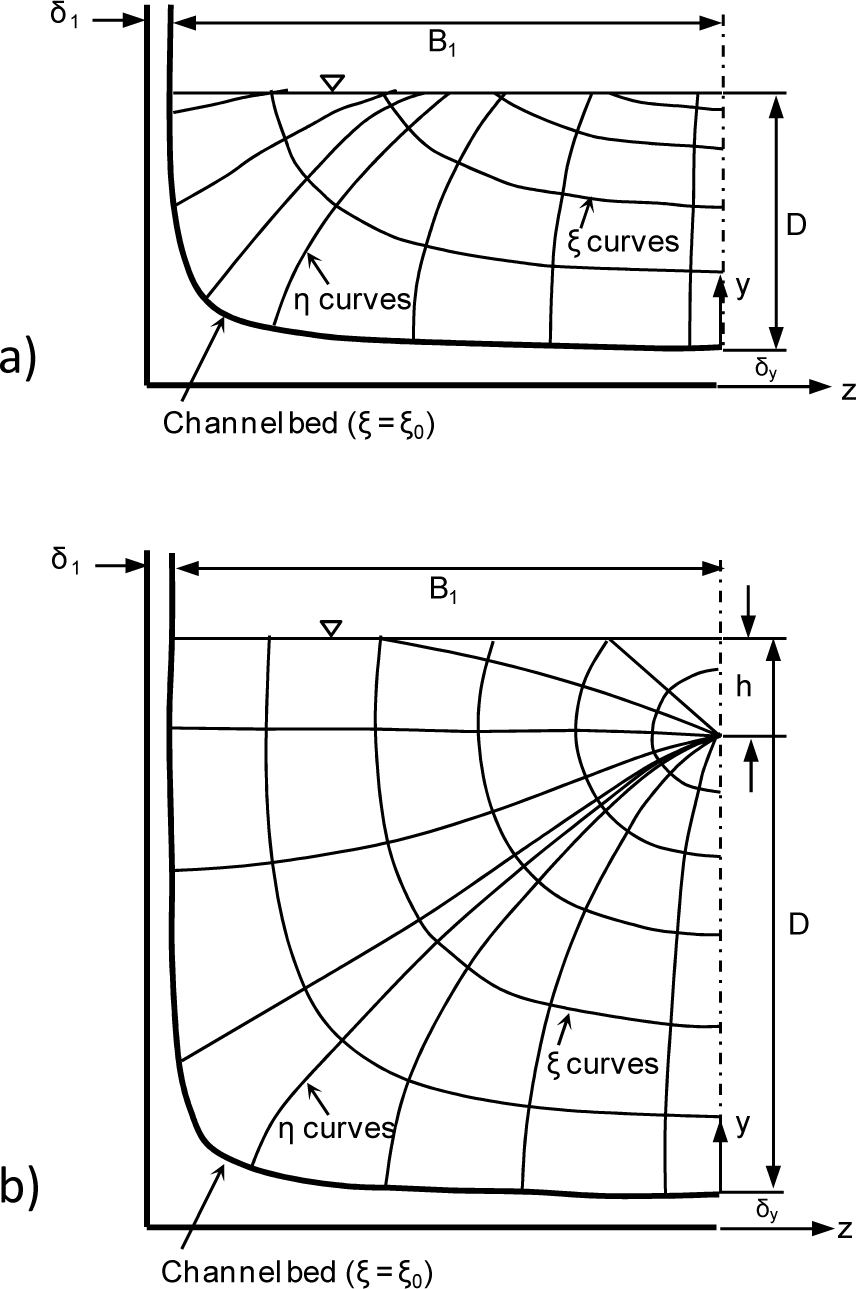
where umax is the cross-sectional maximum point velocity and M is a parameter. In particular, F(u) can be read as the fraction of flow area in which the velocity remains less than or equal to u and is thus quickly and easily identifiable once the isovelocity curves are known. These curves can be plotted using the curvilinear coordinate ξ, expressed as follows by Chiu and Lin [23] and Chiu and Chiou [24] in order to represent different velocity trends in the cross-section:
where Y and Z depend in turn on real spatial coordinates y (vertical) and z (horizontal) according to the relationships shown below:
where D represents the maximum depth in the cross-section and h the depth at which the maximum velocity occurs (h ≥ 0 if below the water surface, h < 0 if above it). The vertical where umax occurs is called the y-axis and D and h are also determined here. The parameters βi, Bi and δi (where i = 1, 2) are respectively the exponent, top width and shift of the zero plane (lateral), which are applied to the left (i = 1) and right (i = 2) of the y-axis. δy is the shift of the zero plane from the bottom (Figure 1).
Based on the curvilinear coordinate ξ, therefore, Chiu [1] proposes expressing the cumulative probability distribution F(u) in the following manner:
where ξmax is the value of ξ in the point where the maximum velocity u = umax, occurs, and ξ0 is the value of ξ in the point (or points) where the velocity u = 0.
By substituting, in the following order, Equation (3) into Equation (2), Equation (2) into Equation (4) and Equation (4) into Equation (1) one obtains an equation that describes the two-dimensional distribution of the velocity within the cross-section:
It is important to highlight that Equation (5) enables us to describe the spatial distribution of the velocity in a generic flow area, albeit at the cost of having to define no fewer than 7 parameters.
In the simplifying assumption that δy is small enough to be considered negligible (δy ≅ 0), ξ0 = 0 when u = 0 and ξmax = 1 for the velocity u = umax and, assuming z = 0, that is, positioned on the vertical y-axis passing through the point where the cross-sectional maximum velocity occurs, Equation (5) is reduced to the following form:
Equation (6) thus has validity on the y-axis, but different authors [25–28] have shown that it is reasonable in practical applications to extend this profile to the generic vertical of a cross-section without having to rely on Equation (5) for the assigned z.
Given the relative simplicity of Equation (6), it is also easy to express the corresponding mean velocity ūi on the i-th vertical:
where uDi is the surface velocity on the i-th vertical and I(M,hi/Di) takes on the following expression:
Finally, again starting from Equation (6), it is possible to put the maximum velocity umax that occurs on the y-axis (and, based on what was observed previously, on the generic vertical as well) in relation with the corresponding surface velocity uD, simply by setting y = D:
The entropy parameter M always appears in the above equations. For a generic river cross-section, an estimate of M is usually derived from the following equation presented by Chiu and Said [15], which puts the maximum velocity umax (observed on the y-axis) in relation with the cross-sectional mean velocity Ū:
where:
Equation (10) has been experimentally validated by several authors [12,25,29–31] using data pairs consisting of Ū and umax, which are distributed around a straight line passing through the origin.
From Equation (10), it is also evident that an estimate of the cross-sectional mean velocity can be obtained immediately once the maximum velocity umax and parameter M are known. It follows that the discharge in the cross-section can be easily estimated by multiplying Ū by the flow area A. It is precisely this aspect which makes Equation (10) a valid alternative to the velocity-area method for estimating discharge, as the only measurement that needs to be made is of the maximum velocity umax, which usually occurs in the upper middle part of the cross-section. In contrast, in the scientific literature, as noted above in the introduction, the parameter M is always estimated from the pairs Ū and umax, where Ū, in particular, is in turn deduced using the velocity-area method, which notoriously entails measuring the point velocity at different depths along a series of verticals whose number will depend on the cross-section size. In short, though Equation (10) is easy to use during the application phase, its parameterization (tied to the estimate of the parameter M) requires the use of the velocity-area method and hence complex, costly measurements that are also dangerous during a flood event. In the following section three alternative methods for estimating the parameter M are presented, which are progressively less cumbersome in terms of velocity data acquisition.
3. Estimation of the Parameter M
Three different methods for estimating the entropy parameter M are proposed. Method 1 requires current-meter measurements for the entire cross-section, while Methods 2 and 3 rely, respectively, on surface velocity measurements alone and the maximum surface velocity alone. The latter methods can thus also be easily applied when “no-contact” measuring techniques are adopted.
3.1. Method 1
Method 1 for estimating the parameter M is based on the equation that links the velocity u to its cumulative probability distribution F(u) within the generic cross-section, as expressed by Equation (1):
The idea underlying Method 1 is the following. Let us suppose that the geometric characteristics of the cross-section, umax and F(u) with variations in u, are known in relation to an assigned flow condition or flood event. In this case, measurements are performed in the same way as when using the velocity-area method and based on these measurements, one can both estimate the maximum velocity umax and trace the isolines of equal velocity with suitable methods of graphic regularization. Given the intrinsic significance of F(u) (percentage of flow area in which the velocity is less than or equal to an assigned value), the function F(u) is actually reconstructed point by point from these isolines. Using this information it is sufficient to choose the value of M which minimizes the deviation between the function F(u) provided by Equation (12) and the one reconstructed point by point from the velocity isolines.
Obviously, this reasoning can be applied with reference either to a single event in which measurements are taken, or a large number of events; in the latter case it will be possible to identify a parameter M enabling Equation (12) to best reproduce the many experimental F(u)s.
It is worth highlighting that, with this method, the characterization of F(u) is independent of the definition of the seven parameters presented in the previous section (see Equations (2)–(4)). However, the number of velocity measurements is the same as required for the application of the velocity-area method. Methods 2 and 3 described in the sections below require a much smaller number of velocity measurements, all of them on the surface.
3.2. Method 2
The application of Method 2 requires knowledge of the cross-section geometry and surface velocity measurements related to one or (preferably) more flow conditions.
The general idea underlying Method 2 is that one can estimate the cross-sectional mean velocity Ū by following two different procedures, both of which solely depend on the entropy parameter M. In this context it is clear that the most appropriate value of the parameter M is the one that renders the two estimates of Ū as close as possible, if not equal. Indeed, it is worth noting that both the procedures, are based on concepts and equations developed within the framework of the entropic method and are well established in the scientific literature. Their reliability has been shown in several papers (e.g., [1,13–16,25,28,31] and thus, it is reasonable that the two procedures provide very similar (if not equal) mean velocity estimations when the most appropriate estimate of the parameter M is used.
In the operational phase, therefore, a preliminary tentative value is fixed for M and then procedures 1 and 2 are carried out as described below.
Procedure 1
The highest of the surface velocity measurements is identified and interpreted as uD relative to the y-axis. Then umax is estimated based on Equation (9) and Φ(M) via Equation (11) by using the tentative value fixed for M. Finally, Ū is estimated by means of Equation (10); it will hereinafter be indicated as Ū1.
Procedure 2
The surface velocities are each interpreted as the surface velocity on the i-th vertical, i.e., uDi, and then transformed into mean velocities via Equation (7) by using the initial tentative value fixed for M. For this purpose, the ratio hi/Di needs to be fixed and this is done using methods described further below.
Once the mean velocities on the different verticals are known, it is possible to estimate the discharge by applying the well known mean section method [32]:
where bi is the distance from an initial datum point to the i-th vertical and Di represents the depth along the i-th vertical. Finally, the cross-sectional mean velocity Ū2 is estimated as a ratio between discharge and flow area.
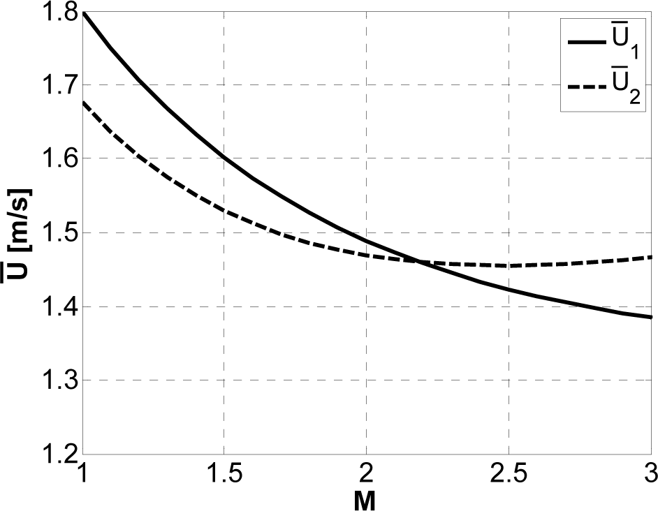
The parameter M sought is the one that makes Ū1 ≅ Ū2. More precisely, in the case of a single flood event, the optimal value of M is the value at which the two aforesaid cross-sectional mean velocities coincide as shown for example in Figure 2; if, on the other hand, one considers N events or flow conditions together, the estimate of the parameter M is performed by minimizing the objective function OF defined as the sum of relative errors between the two mean velocities of the N events:
This OF was selected among several objective functions since it allows to properly take into considerations both large, medium and small flood events and the corresponding mean flow velocity errors.
Before concluding, it is important to describe how to quantify the ratio between hi (depth of the point where the maximum velocity of the i-th vertical occurs) and Di (water depth on that vertical) for each vertical, including the y-axis itself. Based on information drawn from the scientific literature, there are two possible approaches:
Approach A—the hi/Di ratio is expressed as a function of M according to the relationship provided by Chiu and Tung [17], i.e.,:
This relationship was proposed in reference to the y-axis and its validity has been ascertained only for large rivers. For the application of Method 2, it is assumed that the validity of this equation can also be extended to the generic vertical.Approach B—the hi/Di ratio is assumed to be constant across all verticals and independent of M, as proposed by Alessandrini et al. [28]. The actual value of this ratio can be deduced on the basis of a series of observations relating to a number of events and a number of verticals [26].
3.3. Method 3
Method 3 is a variant of Method 2, but can be carried out even more rapidly thanks to the fact that the sampling is narrowed to the maximum surface velocity uD which typically is located near the middle of the channel ([33,34]) and thus it can be sampled by carrying out very few measurements in that portion of the channel; as in Method 2, the hydrometric cross-section geometry is assumed to be known.
Similarly to what is seen for the case of Method 2, the mean velocities Ū1 and Ū2 are calculated by following two distinct procedures. The one for calculating Ū1 is the same as in Method 2, since the available velocity uD is interpreted as belonging to the y-axis, whereas the procedure for calculating Ū2 differs in the initial step: in fact, considering that multiple surface velocity measurements are not available, but only the maximum one, their distribution is surmised by relying on particular analytic functions that depend on the only available measurement. Indeed, based on field data it is shown in several papers that the surface velocities can be properly approximated through functions such as a parabola or an ellipse. Moramarco et al. [27,35] justified the validity of these equations for fitting the surface velocities through the Chezy’s formula. Specifically, in this study the following functions are used: (a) parabolic function type 1: two parabolas are drawn, the vertex of both coinciding with the only point of measurement and passing through the left and right banks; (b) parabolic function type 2: two parabolas are drawn, with their vertices on the banks and each passing through the point of measurement of the maximum velocity; (c) elliptic function: two branches of an ellipse are drawn, both passing through the point of measurement of the maximum velocity and through the banks; (d) cubic function: two cubic parabolas are drawn, with their vertex on the banks and both passing through the only available point of measurement. With specific reference to the parabolic functions it is worth noting that both type 1 and 2 ensure that the maximum velocity provided by the parabolic function coincides with the point of measurement of the maximum velocity. Indeed, a third type of parabolic function there could exist, i.e., one parabola passing through the three points, the two banks and the measured maximum velocity point, but in such a case the vertex of the parabola, and thus maximum velocity provided by the parabola itself, would not coincides with the measured maximum velocity if the point of measurement of the maximum velocity is not located exactly in the middle between the two banks, and thus this this type of parabola was not considered in the numerical application.
The surface velocities uDi calculated for hypothetical verticals (no longer observed ones, as in Method 2) are converted into mean velocities along these (calculation) verticals using Equation (7). From this point onward, the procedure for calculating Ū2 follows the same steps as described for Method 2.
4. Case Study
The three proposed methods for estimating the entropy parameter M were applied and verified using data relating to the Ponte Nuovo gauging station located along the Tiber River (central Italy). The basin closed at Ponte Nuovo drains an area of about 4,135 km2 and is equipped with a cableway that enables velocity measurements to be performed using a current meter on different verticals and at different depths. The station is also equipped with a level gauge and, since 2000, an ultrasonic flowmeter which provides continuous discharge recordings for a broad range of flow conditions.
The dataset used consists of N = 55 flood events recorded between December 1982 and May 2007; the number of measurement verticals sampled for each event ranges between 7 and 14, depending on the entity of flooding, and at least 4 point velocity measurements were performed for each vertical.
Table 1 shows the ranges of the number of verticals nv, the number nmis of point velocity measurements made and the main hydraulic parameters—discharge Q, water depth D on the y-axis, cross-sectional mean velocity Ū, cross-sectional maximum velocity umax and depth h at which the maximum velocity occurs—for the N = 55 events. In particular, the discharge Q was calculated on the basis of point velocity measurements using a variant of the mean-section method (see Equation (13)), and the cross-sectional mean velocity Ū was obtained by dividing this discharge value by the flow area; finally, the maximum sampled velocity umax is interpreted as the maximum cross-sectional velocity umax for the event considered [1].
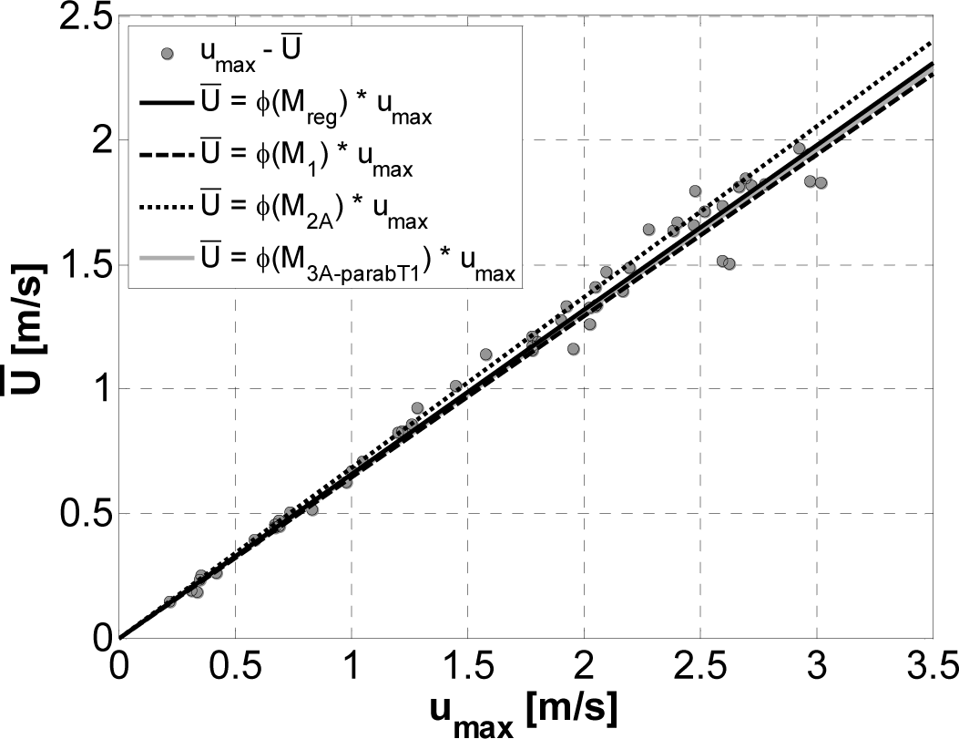
As can be seen from Table 1, the 55 events considered are characterized by a broad range of discharge values, from 5.76 to 541.58 m3/s, with corresponding mean velocities ranging between 0.15 and 1.97 m/s and maximum velocities between 0.22 and 3.00 m/s. It is moreover interesting to observe that umax occurred on the surface (h = 0) in 35 out of the total 55 flood events considered, and in 9 of the remaining 20, the maximum cross-sectional velocity occurred in any case less than 36 cm below the free surface. In general, therefore, the maximum velocity almost always occurs on or in proximity to the surface. On the basis of the 55 pairs of umax-Ū values, finally, the existence of a direct proportionality between the two above-mentioned velocities (see Equation (10) and Figure 3) was verified, and the value of Φ(M) estimated by means of a least-squares linear regression, which gave a result of 0.66, corresponding (Equation (11) to a value of M equal to 2.06. By looking at Figure 3 it is also worth noting that all the pairs of umax-Ū values pertaining to 55 flood events occurred over a very long time lapse, from 1982 to 2007 (25 years, see also Table 1) are all well approximated by the entropic linear relationship featuring a single/constant M value, thus confirming that this parameter can be assumed time invariant. The Φ(M) = 0.66 and M = 2.06 values were taken as reference values for the purpose of comparing the corresponding values given by the three new methods proposed.
5. Analysis and Discussion of the Results
5.1. Analysis and Discussion of the Results of Method 1
In the case of Method 1 (see Section 3.1) the value of the entropy parameter M was determined considering all of the N = 55 events together, so that for each event the cumulative probability distribution of the velocity F(u) of Equation (12) would best reproduce the experimental functions F(u) obtained after the isovelocity curves had been plotted. For this purpose the “fmincon” function provided in the Matlab™ optimization toolbox was used so as to minimize the sum of squared deviations between the F(u) of Equation (12) and the experimental ones. The value of M obtained was 1.87, close to the reference value of 2.06 obtained with the linear regression of umax-Ū. The difference is further reduced if one considers Φ(M), which takes on a value of 0.65 versus the reference value of 0.66 (see also Figure 3). This is very encouraging, since what counts for the making the step from umax to Ū (and thus for the discharge estimate) is precisely the function Φ(M) which is not very sensitive to M, thus producing a robust estimate of the mean flow velocity (see Equation (10)).
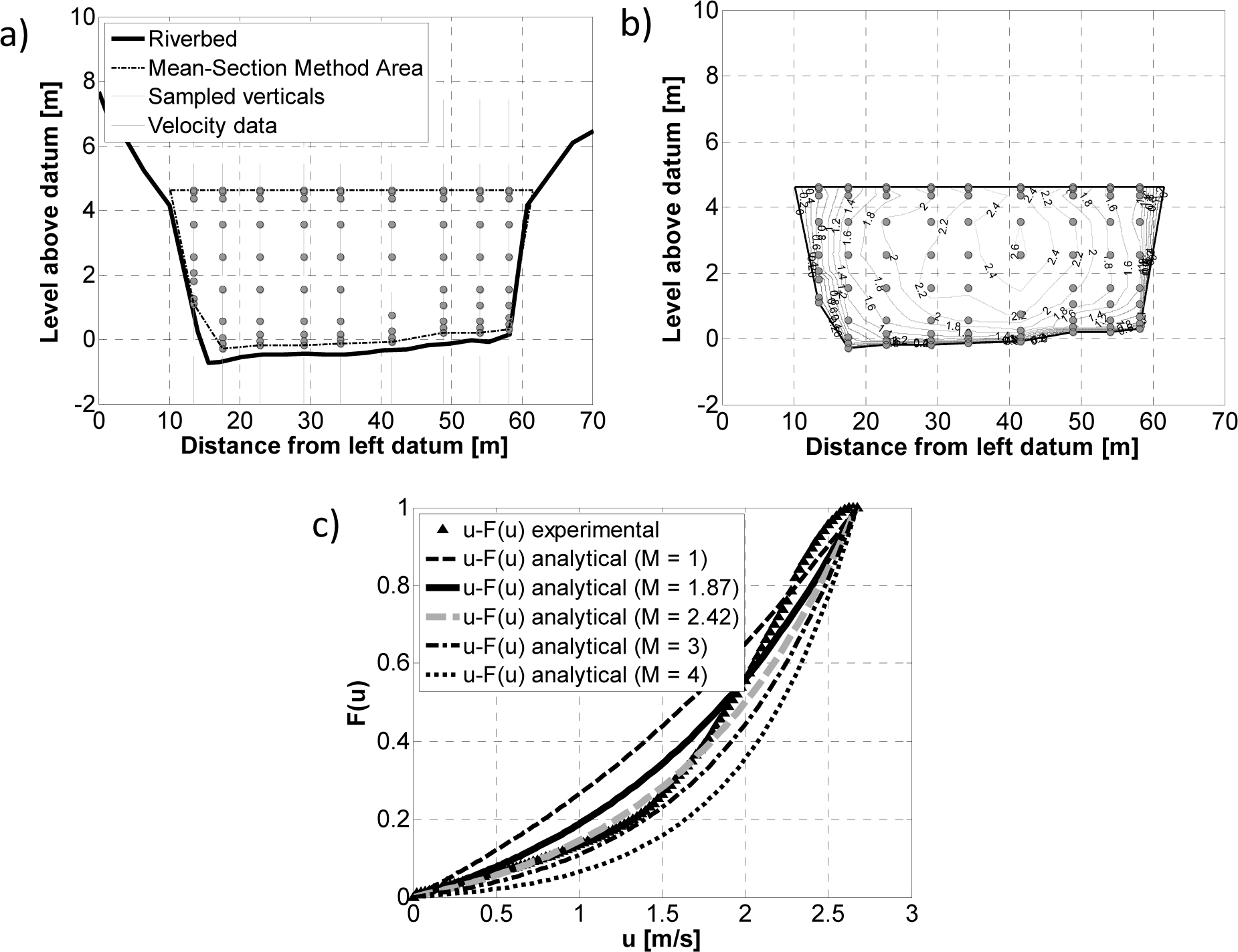
The isovelocity curves for each event, necessary for calculating the experimental distributions F(u), were plotted using the point velocity measurements over different verticals at different depths; this was done by performing a two-dimensional linear interpolation and joining the points with an equal velocity from u = 0 to u = umax, considering very small steps of 0.025 m/s. On the basis of these curves, the experimental function F(u) was obtained by calculating the fraction of flow area in which the velocity is less than or equal to a value u, with u = 0, 0.025, 0.05, …, umax. Figure 4 illustrates, by way of example, the different steps of Method 1 for the flood event of April 20, 2004: in particular, it shows the measurements made during the event (Figure 4a), the isovelocity curves obtained as a result of the two-dimensional interpolation (Figure 4b, in which the curves are displayed with ∆u = 0.2 m/s) and the experimental probability distribution function F(u) obtained (c). This distribution is also compared with the one provided by Equation (12) for different values of M (M = 1, 3, 4), including both the value M =1.87 obtained from the calibration over N = 55 events, and the value M = 2.42 which best reproduces the experimental function F(u) of the single event of 20 April 2004. Incidentally, the maximum velocity umax of Equation (12) was assumed to be equal to the highest of the velocities measured in the event considered (see Table 1).
As can be observed for this event, as well as for many of the other 54 events, there is a point in the experimental function where the curvature changes; the curve of Equation (12), by its very nature, does not show it, irrespective of the value of M, and it may be noted that the convexity increases with increases in the value of this parameter. In any case, the value M = 1.87, which best reproduces the experimental functions of all N = 55 events, also in specific reference to the single event represented here, results in a cumulative probability function, given by Equation (12), which is a good approximation of the experimental one.
Before concluding, it is worth considering a further point. As already said, Method 1 relies on velocity measurements made on different verticals at different depths and therefore, in particular, measurements taken on a vertical that can be assumed as representative of the y-axis. Focusing on this latter information, it is easy to understand that by using Equation (6) (where at this point the pairs u-y, umax, h and D are known) it is possible to develop a method for estimating the entropy parameter M that would consist in selecting the value providing the best fit to the observed velocity profile. This method for estimating M would have an advantage over Method 1 discussed above in that it would require a smaller number of measurements: indeed, the latter would be concentrated on the y-axis alone. This method was not included, however, among those proposed, as its application led to unsatisfactory results. In fact, the values of M obtained using this potential method were always much larger than the reference value. The reason for this is that if a single vertical (the y-axis) is considered, the information about the spatial distribution of velocity in the flow area is lost, which concerns the entire cross-section and which the parameter M itself refers to (in this regard, see Equation (1)). In other words, M is a cross-sectional parameter and seeking to estimate it on the basis of information concentrated on only one vertical would signify going against its very meaning. Precisely for this reason, the three methods presented and discussed here, despite involving a progressively smaller number of measurements, are all structured on a cross-sectional basis, taking into account, therefore, the entire spatial distribution of the velocity in the flow area.
5.2. Analysis and Discussion of the Results of Method 2
With Method 2 the value of the entropy parameter M was determined considering the N = 55 events together and minimizing the objective function of Equation (14). The estimation was repeated using both approaches to quantify the hi/Di ratio, A and B.
In particular, in the case of A, where the hi/Di ratio is a function of the entropy parameter, a value of M = 2.43 is obtained, and a consequent value of the function Φ(M) = 0.69.
In the case of B, on the other hand, hi/Di was assigned a fixed constant value of 0.20, which resulted from the averaging of the verticals of all N = 55 events; such a low mean value is understandable considering that, as previously observed, the maximum point velocity occurred on the surface in the majority of events (see Table 1) and the same behavior was also observed in the verticals adjacent to the y-axis. The resulting value of the entropy parameter M was 1.91, leading to a value of the function Φ(M) = 0.65.
In the case of A the value of M = 2.43 is slightly overestimated compared to the reference value (M = 2.06), but it results nonetheless in an extremely small percentage error in the value of the function Φ(M), less than 5% (Φ(M) = 0.69 vs. Φ(M) = 0.66 see also Figure 3); in the case of B, on the other hand, the values of M = 1.91 and Φ(M) = 0.65 are substantially equivalent to the reference ones obtained through linear regression. In any case, it is important to remember that the relationship of Equation (15) was originally defined with specific reference to the y-axis and derived on the basis of a vast set of both laboratory and field data collected during different flood events and for different regimes. In particular, this relationship provides a value of hi/Di that is close to 0.6 for considerably low values of M (M = 1), whereas the ratio approaches zero when the values of M are very high (M = 5.6). Remembering that at the Ponte Nuovo gauging station the maximum velocity on the y-axis and in a large part of the other verticals often occurred on the surface, having hi/Di ratios close to 0 it is comprehensible why the relationship of Equation (15) results in a (slight) overestimate of M.
5.3. Analysis and Discussion of the Results of Method 3
Method 3 is nearly identical to Method 2; the only substantial difference lies in the fact that in the former only the maximum surface velocity is considered to be available. Hence our reliance on particular geometric functions to derive other surface velocities associated with hypothetical verticals.
In this case as well, the entropy parameter M was estimated considering the N = 55 events together and using both approaches A and B to quantify the hi/Di ratio.
Table 2 shows the values of M and Φ(M) obtained using each of the 4 geometric functions considered and for both methods of quantifying the hi/Di ratio.
One can observe that, irrespective of how the hi/Di ratio is derived, M varies markedly, from 1.5 to 4, but the function Φ(M) shows more limited variability: in fact, depending on the geometric function used, the values of Φ(M) remain between 0.60 and 0.77, in the vicinity of the reference value 0.66 obtained through regression, and corresponding to a percentage error of about 10%–15%.
In both cases A and B, the parabolic function type 2 (two parabolas with vertices on the banks and passing through the point of measurement of the maximum velocity) and the elliptic one provide the lowest and highest values of M, respectively: this is in agreement with the definition often found in the literature, where the entropy parameter is understood as a “measure of the uniformity of the velocity distribution in a cross-section” [1] since, for any given event, the parabolic function type 2 is the one that most accentuates the variability in the velocity in the central area, whereas the velocity values provided by the elliptic curve tend to be more uniform in the central area of flow.
Summing up, Method 3 has the undoubted advantage of requiring only one velocity measurement, but on the other hand it entails using a particular geometric function in order to characterize the pattern of surface velocities: the choice of this function will influence the accuracy of the estimate of M and, to a lesser extent, Φ(M), so preliminary surface measurements should be performed to identify the optimal function. In the specific case considered in this study, the parabolic function type 1 proved to be the most suitable for characterizing the surface velocity distribution; this is in agreement with the results obtained in previous studies [25], and enables us to achieve a very accurate estimate of Φ(M) (see Figure 3).
6. Discussion and Conclusions
Three methods are proposed for estimating the entropy parameter M in a river cross-section. These methods represent a valid alternative to the standard approach based on the linear regression of a considerable number of pairs of values umax-Ū, which are in turn estimated using the velocity-area method.
The three methods differ not only in their approach, but also (and above all) in the amount of information/data required for their application, which progressively decreases going from Method 1 to Method 3.
The proposed methods underwent validation on the basis of numerous field velocity measurements taken at the Ponte Nuovo gauging station on the Tiber River during flood events occurring between 1982 and 2007. The robustness of all 3 methods was confirmed, though the accuracy of the estimate of the entropy parameter M falls slightly as the amount of information/field measurements used to estimate it decreases.
In fact, Method 1, in which the estimate of M is based on reproducing the cumulative velocity distribution function associated with a flood event, provides values of M and Φ(M) that are nearly identical to the reference values; however, it requires costly sampling of velocities across the entire hydrometric cross-section, from the surface to the bottom. Though this method offers the advantage of rendering F(u) independent of the determination of the seven parameters characterizing the two-dimensional velocity distribution based on the curvilinear coordinate ξ (see Equations (2)–(4)), in terms of sampling it is equally as cumbersome as the velocity-area method.
In Methods 2 and 3, in contrast, the estimate of M is based on reproducing the cross-sectional mean velocity Ū by following two different procedures, both of which rely on the entropy parameter M (alone), and looking for the value of M that brings the two estimates of Ū as close together as possible. Neither method requires any velocity measurements below the surface, and this enables a significant reduction in the times and costs of gauging campaigns. In particular, while Method 2 entails measuring the surface velocity across the entire top width, Method 3 reduces sampling to a measurement of the maximum surface velocity alone. It is also important to observe that in both cases the maximum cross-sectional velocity is estimated on the basis of the maximum surface velocity and relying on the entropic velocity profile.
Both Method 2 and Method 3 provide, on the whole, a good estimate of the entropy parameter M and—most importantly—values of Φ(M) that are close to the reference values, though in the case of Method 3, the accuracy depends on which geometric function is used to approximate the surface velocity distribution. In practice, by using methods that require less data to estimate the entropy parameter, the accuracy of the estimation of M slightly decreases and, particularly in the case of Method 3, the accuracy is affected by the choice of the geometric function used to characterize the pattern of surface velocities. However, it is shown that a less accurate estimate of M hardly affects the Φ(M) estimate, and with specific reference to Method 3, the accuracy obtained by using the parabolic function type 1, already indicated in previous studies as the most suitable for characterizing the surface velocity distribution, is very good.
Finally, a clear advantage can be derived from using the latter two methods to monitor river discharge, considering that no-contact radar sensors and/or satellite data are now available for the measurement of surface velocities, which both reduces the times and costs of taking measurements and ensures the maximum safety of personnel.
Acknowledgments
The authors wish to thank Umbria Region, Department of Environment, Planning and Infrastructure, for providing Tiber River basin data.
Author Contributions
Each of the authors contributed to the design, analysis, and writing of the study.
Conflicts of Interest
The authors declare no conflict of interest.
References
- Chiu, C.L. Entropy and 2-D velocity in open channels. J. Hydraul. Eng 1988, 114, 738–756. [Google Scholar]
- Jaynes, E.T. Information theory and statistical mechanics. I. Phys. Rev 1957, 106, 620–630. [Google Scholar]
- Leopold, L.B.; Langbein, W.B. The Concept of Entropy in Landscape Evolution; Government Printing Office: Washington, DC, USA, 1962; pp. 1–20. [Google Scholar]
- Davy, B.W.; Davies, T.R.H. Entropy concepts in fluvial geomorphology: A reevaluation. Water Resour. Res 1979, 15, 103–106. [Google Scholar]
- Sonuga, J.O. Principal of maximum entropy in hydrologic frequency analysis. J. Hydrol 1972, 17, 177–191. [Google Scholar]
- Jowitt, P.W. The extreme-value type-I distribution and the principle of maximum entropy. J. Hydrol 1979, 42, 23–38. [Google Scholar]
- Singh, V.P.; Marini, G.; Fontana, N. Derivation of 2D power-law velocity distribution using entropy theory. Entropy 2013, 15, 1221–1231. [Google Scholar]
- Fontana, N.; Marini, G.; de Paola, F. Experimental assessment of a 2-D entropy-based model for velocity distribution in open channel flow. Entropy 2013, 15, 988–998. [Google Scholar]
- Chiu, C.L. Entropy and probability concepts in hydraulics. J. Hydraul. Eng 1987, 113, 583–600. [Google Scholar]
- Chen, C.Y.; Kuo, J.J.; Yu, R.S.; Liao, J.Y.; Yang, C.H. Discharge estimation in a Lined Canal Using Information Entropy. Entropy 2014, 16, 1728–1742. [Google Scholar]
- Chiu, C.L. Application of entropy concept in open channel flow study. J. Hydraul. Eng 1991, 117, 615–628. [Google Scholar]
- Xia, R. Relation between mean and maximum velocities in a natural river. J. Hydraul. Eng 1997, 123, 720–723. [Google Scholar]
- Chiu, C.L. Velocity distribution in open channels. J. Hydraul. Eng 1989, 115, 576–594. [Google Scholar]
- Chiu, C.L.; Murray, D.W. Variation of velocity distribution along non-uniform open-channel flow. J. Hydraul. Eng 1992, 118, 989–1001. [Google Scholar]
- Chiu, C.L.; Abidin Said, C.A. Maximum and mean velocities and entropy in open-channel flow. J. Hydraul. Eng 1995, 121, 26–35. [Google Scholar]
- Moramarco, T.; Singh, V. Formulation of the Entropy Parameter Based on Hydraulic and Geometric Characteristics of River Cross Sections. J. Hydrol. Eng 2010, 15, 852–858. [Google Scholar]
- Chiu, C.L.; Tung, N. Maximum Velocity and Regularities in Open-Channel Flow. J. Hydraul. Eng 2002, 128, 390–398. [Google Scholar]
- Costa, J.E.; Cheng, R.T.; Haeni, F.P.; Melcher, N.; Spicer, K.R.; Hayes, E.; Plant, W.; Hayes, K.; Teague, C.; Barrick, D. Use of radars to monitor stream discharge by noncontact methods. Water Resour. Res 2006, 42. [Google Scholar] [CrossRef]
- Fulton, J.; Ostrowski, J. Measuring real-time streamflow using emerging technologies: Radar, hydro-acoustics, and the probability concept. J. Hydrol 2008, 357, 1–10. [Google Scholar]
- Bjerklie, D.M.; Dingman, S.L.; Vorosmarty, C.J.; Bolster, C.H.; Congalton, R.G. Evaluating the potential for measuring river discharge from space. J. Hydrol 2003, 278, 17–38. [Google Scholar]
- Romeiser, R.; Sprenger, J.; Stammer, D.; Runge, H.; Suchandt, S. Global current measurements in rivers by spaceborne along-track InSAR, In Proceedings of the IEEE IGARSS-2005 International Geosciences and Remote Sensing Symposium, Seoul, South Korea, 25–29 July 2005.
- Alsdorf, D.E.; Rodríguez, E.; Lettenmaier, D.P. Measuring surface water from space. Rev. Geophys 2007, 45. [Google Scholar] [CrossRef]
- Chiu, C.L.; Lin, G.F. Computation of 3-D flow and shear in open channels. J. Hydraul. Eng 1983, 109, 1424–1440. [Google Scholar]
- Chiu, C.L.; Chiou, J.D. Structure of 3-D flow in rectangular open channels. J. Hydraul. Eng 1986, 112, 1050–1068. [Google Scholar]
- Moramarco, T.; Saltalippi, C.; Singh, V.P. Estimation of mean velocity in natural channels based on Chiu’s velocity distribution equation. J. Hydraul. Eng 2004, 9, 42–50. [Google Scholar]
- Corato, G.; Moramarco, T.; Tucciarelli, T. Discharge estimation combining flow routing and occasional measurements of velocity. Hydrol. Earth Syst. Sci 2011, 15, 2979–2994. [Google Scholar]
- Moramarco, T.; Saltalippi, C.; Singh, V.P. Velocity profiles assessment in natural channels during high floods. Hydrol. Res 2011, 42, 162–170. [Google Scholar]
- Alessandrini, V.; Bernardi, G.; Todini, E. An operational approach to real-time dynamic measurement of discharge. Hydrol. Res 2013, 44, 953–964. [Google Scholar]
- Moramarco, T.; Saltalippi, C. Stima della velocità media in sezioni di un corso d’acqua naturale, In Proceedings of XXVIII National Conference on Hydraulics and Hydraulic Structures, Potenza, Italy, 16–19 September 2002; pp. 263–274.
- Ardiclioglu, M.; de Araujo, J.C.; Seturk, A.I. Applicability of velocity distribution equations in rough-bed open channel flow. Houille Blanche 2005, 4, 73–79. [Google Scholar]
- Ammari, A.; Remini, B. Estimation of Algerian rivers discharges based on Chiu’s equation. Arab. J. Geosci 2010, 3, 59–65. [Google Scholar]
- Hydrometry, Measurement of Liquid Flow in Open Channels Using Current-Meters or Floats, UNI EN ISO 748. 2008.
- Chen, C.Y.; Chiu, L.C. A fast method of flood discharge estimation. Hydrol. Processes 2004, 18, 1671–1684. [Google Scholar]
- Corato, G.; Melone, F.; Moramarco, T.; Singh, V.P. Uncertainty analysis of flow velocity estimation by a simplified entropy model. Hydrol. Processes 2014, 28, 581–590. [Google Scholar]
- Moramarco, T.; Corato, G.; Melone, F.; Singh, V.P. An entropy-based method for determining the flow depth distribution in natural channels. J. Hydrol 2013, 497, 176–188. [Google Scholar]


| Date | nv | nmis | Q | Ū | D | umax | h |
|---|---|---|---|---|---|---|---|
| [m3/s] | [m/s] | [m] | [m/s] | [m] | |||
| 1982–2007 | 7–14 | 46–108 | 5.76–541.58 | 0.15–1.97 | 0.94–6.64 | 0.22–3.00 | 0.00–2.94 |
| Approach | Parabolic Function
| Elliptic Function | Cubic Function | |
|---|---|---|---|---|
| Type 1 | Type 2 | |||
| A | M = 1.96 | M = 1.71 | M = 4.03 | M = 3.11 |
| Φ = 0.65 | Φ = 0.64 | Φ = 0.77 | Φ = 0.73 | |
| B | M = 1.47 | M = 1.26 | M = 3.92 | M = 2.70 |
| Φ = 0.62 | Φ = 0.60 | Φ = 0.77 | Φ = 0.70 | |
© 2014 by the authors; licensee MDPI, Basel, Switzerland This article is an open access article distributed under the terms and conditions of the Creative Commons Attribution license (http://creativecommons.org/licenses/by/3.0/).
Share and Cite
Farina, G.; Alvisi, S.; Franchini, M.; Moramarco, T. Three Methods for Estimating the Entropy Parameter M Based on a Decreasing Number of Velocity Measurements in a River Cross-Section. Entropy 2014, 16, 2512-2529. https://doi.org/10.3390/e16052512
Farina G, Alvisi S, Franchini M, Moramarco T. Three Methods for Estimating the Entropy Parameter M Based on a Decreasing Number of Velocity Measurements in a River Cross-Section. Entropy. 2014; 16(5):2512-2529. https://doi.org/10.3390/e16052512
Chicago/Turabian StyleFarina, Giulia, Stefano Alvisi, Marco Franchini, and Tommaso Moramarco. 2014. "Three Methods for Estimating the Entropy Parameter M Based on a Decreasing Number of Velocity Measurements in a River Cross-Section" Entropy 16, no. 5: 2512-2529. https://doi.org/10.3390/e16052512