Measuring Instantaneous and Spectral Information Entropies by Shannon Entropy of Choi-Williams Distribution in the Context of Electroencephalography


Abstract
: The theory of Shannon entropy was applied to the Choi-Williams time-frequency distribution (CWD) of time series in order to extract entropy information in both time and frequency domains. In this way, four novel indexes were defined: (1) partial instantaneous entropy, calculated as the entropy of the CWD with respect to time by using the probability mass function at each time instant taken independently; (2) partial spectral information entropy, calculated as the entropy of the CWD with respect to frequency by using the probability mass function of each frequency value taken independently; (3) complete instantaneous entropy, calculated as the entropy of the CWD with respect to time by using the probability mass function of the entire CWD; (4) complete spectral information entropy, calculated as the entropy of the CWD with respect to frequency by using the probability mass function of the entire CWD. These indexes were tested on synthetic time series with different behavior (periodic, chaotic and random) and on a dataset of electroencephalographic (EEG) signals recorded in different states (eyes-open, eyes-closed, ictal and non-ictal activity). The results have shown that the values of these indexes tend to decrease, with different proportion, when the behavior of the synthetic signals evolved from chaos or randomness to periodicity. Statistical differences (p-value < 0.0005) were found between values of these measures comparing eyes-open and eyes-closed states and between ictal and non-ictal states in the traditional EEG frequency bands. Finally, this paper has demonstrated that the proposed measures can be useful tools to quantify the different periodic, chaotic and random components in EEG signals.1. Introduction
Since the works of Kotelnikov and Shannon [1,2], it has been proved that the information provided by an event associated with the inverse of the probability of an event occurrence has been extremely useful for its significance and inherent conceptual simplicity.
The classical Shannon entropy measures the average information provided by a set of events and proves its uncertainty. This measure is shown as a natural candidate for quantifying the complexity of a signal. Also the level of chaoticity may be measured using entropy; therefore higher entropy represents higher uncertainty and a more irregular behavior of the signal. Moreover, if noise is added to an ordered signal the uncertainty increases and the entropy is also increased. Entropy can even explain how linked complex systems interact and exchange information. The quantification of the magnitude of this information becomes a goal in the study of biological signals.
The entropy estimation consists in calculating the probability of events that occur in time signals and in obtaining a reliable average value of the information provided by each of these events. The evolution of the entropy of a signal with respect to time, calculated from the instantaneous information of a window that slides over the signal, is a smoothing of the sequence of instantaneous information because the entropy is the average value of the information in this window.
The purpose of this paper is both to avoid this low-pass filtering inherent in the calculation of the entropy and to obtain instantaneous values of this measure. The time-frequency representation (TFR) technique is suited to achieve both aims. TFR generalizes the concept of the time and frequency domains to a joint time—frequency function that indicates how the frequency content of a signal changes over time [3,4]. Complexity studies based on entropy functional take advantage of the analogy between signal energy densities and probability densities [5]. While the instantaneous and spectral amplitudes behave as one-dimensional densities of signal energy in time and in frequency, TFR tries to act as 2-dimensional energy densities in both time and frequency [6].
In this paper, we investigate new measures that quantify the complexity and information content of a signal. Selecting time and frequency functions that satisfy marginal properties, one can assume that the energy density of a signal in one instant (or instantaneous power of the signal) is given by the entropy associated with the frequency components of the signal at this time instant (or instantaneous entropy). By similar reasoning, an equivalent measure can be obtained in the frequency domain (spectral information entropy). Thus, a different way to calculate the information in the TFR by estimating a probability density function of a signal either in time or in frequency domain is proposed in this paper. In a similar study, Baraniuk [6] discussed the calculation of the logarithms of Shannon expression with negative value of TFR. In this work this problems is avoided since the probability density of the TFR always contains positive values. Our proposed methodology is based on the original concept of information defined as the logarithm of the inverse value of a probability. This permits to make a comparison with traditional Shannon entropy.
The Choi-Williams distribution (CWD) [3] is a type of Time-Frequency Representation (TFR) whose properties facilitate the purpose of this work. Four novel indexes are defined on the CWD: (1) partial instantaneous entropy, calculated as the entropy of the CWD with respect to time by using the probability mass function at each time instant taken independently; (2) partial spectral information entropy, calculated as the entropy of the CWD with respect to frequency by using the probability mass function of each frequency value taken independently; (3) complete instantaneous entropy, calculated as the entropy of the CWD with respect to time by using the probability mass function of the entire CWD; (4) complete spectral information entropy, calculated as the entropy of the CWD with respect to frequency by using the probability mass function of the entire CWD.
These indexes are tested on synthetic time series that simulate signals in which different behaviors (periodic, chaotic and random) are combined and on a dataset of electroencephalographic (EEG) signals recorded in different states (eyes-open, eyes-closed, ictal and non-ictal activity). For this analysis, EEG signals are selected since they are generated by nonlinear deterministic processes with nonlinear coupling interactions between neuronal populations [7].
2. Methodology
2.1. Time-Frequency Representation
CWD (1) is obtained by convoluting the Wigner distribution (WD) (2) and the Choi-Williams exponential (3) [3,8]:
The spectral power is defined as:
Choosing an adequate parameter σc, the function (3) is able to reduce WD cross-terms and preserve the properties of the WD, such as the marginal properties and instantaneous frequency. In this work, σc was set to 0.005 [8]. The. was normalized by the total power calculated as the area under SpPow.
2.2. Shannon Entropies
Entropy can express the mean of information that an event provides when it takes place, the uncertainty about the outcome of an event and the dispersion of the probabilities with which the events take place. Let X be a discrete random variable which takes a finite number of posble values x1, x2, x3…, xn with probabilities P(1), P(2), P(3)…, P(n) respectively, such that P(i) ≥ 0, i = 1, 2, 3…n,; Shannon entropy (Entr) is defined as:
where n is the number of analyzed samples.
2.3. Instantaneous Entropy and Spectral Information Entropy
The probability mass function (PMF) was defined for a time instant tk with respect to frequency as pTPMF (tk, i) = PCWD(CWDi(t, f) | t = tk)and for frequency value fk with respect to time as pFPMF (i, fk) = PCWD(CWDi(t, f) | f = fk), after the quantization of the CWD(tk,f) and CWD(t,fk), respectively, in n=32 equidistant levels. In this work, a time range of 0 < t < 200 s and a frequency bandwidth of 0 < f < 60 Hz were taken into account.
The two distributions, quantization-time pTPMF (t, i) and quantization-frequency pFPMF (i, f), were obtained for each time instant and frequency value for the entire time 0 < tk < 200 s and bandwidth 0 < fk < 60 Hz. In this way, the two distributions represent partial distribution of PFM with respect to time or to frequency, since in each time instant (tk) and frequency value (fk) the PMF is only related to that time instant (tk) or frequency value (fk). In a similar way, the complete PMF distribution quantization-time and quantization-frequency were calculated as cTPMF (t, i) = PCWD(CWDi(t, f) | 0 < t < 200 s)and cFPMF (i, f) = PCWD(CWDi(t, f) | 0 < f < 60 Hz), respectively, after the quantization of the CWD(t,f) in n = 32 equidistant levels.
From this proposed methodology, new indexes were defined:
Partial instantaneous entropy:
Partial spectral information entropy:
Complete instantaneous entropy:
Complete spectral information entropy:
3. Analyzed Data
3.1. Synthetic Signals
In order to study the performances of the pInstEntr, pSpInfEntr, cInstEntr, cSpInfEntr applied to different types of signals, a set of simulated signals were designed:
- (1).
A periodic signal was generated adding a frequency component (Fi) every 25 s, in this way the first 25 s of the signal has 1 frequency component and the last 25 s has 8 frequency components. The added frequencies were respectively Fi = [0.5;1;2;5;10;20;30;50] Hz. The amplitude of each frequency component was As = 1/NF, where 1 ≤ NF ≤ 8 is the number of the frequency components.
- (2).
A MIX process, used in previous studies [9–11], was defined as MIX = (1 − z)x + zy, where z is a random variable that is equal to 1 with probability p and equal to 0 with probability 1−p, x is a periodic sequence with a frequency component of 10 Hz, and y is a standard uniformly distributed variable on [−√3,√3]. The synthetic signal was based on a MIX process whose parameter p varied linearly from 0.9 to 0.1. Hence, this sequence, evolved from randomness to periodicity.
- (3).
The same MIX process of 2) using as y the Hx obtained from Henon map [12] with chaotic behavior (10), using the canonic values a = 1.4 and b = 0.3, and taking Hx(0) = 0.5 and Hy(0) = 0.5 as initial conditions. Hence, this sequence evolved from chaos to periodicity.
- (4).
The same MIX process of (3) using as y a Henon map with chaotic behavior and as x the standard uniformly distributed variable on [−√3,√3]. Hence, this sequence evolved from chaos to randomness.
All synthetic signals had a length of 200 s and a sampling frequency of 128 Hz. For each synthetic signal, mean (m) of cInstEntr, pInstEntr and the signal entropy Entr were calculated with respect to time in windows of 1 s. The cSpInfEntr and pSpInfEntr and the spectral power of the CWD was also calculated for each signal.
3.2. Real EEG Recordings
A freely available EEG dataset was used for validation [13]. This dataset contains 100 single channel EEG segments of 23.6 s recorded with the same amplifier system, using an average common reference with a sampling rate of 173.6 Hz. The dataset was divided in five different sets (A, B, C, D, E). Sets A and B contain surface EEG signals recorded from five healthy volunteers who were relaxed in an awake state. Whereas the subjects had their eyes open during the recording of the EEG in set A, the EEG signals of dataset B were acquired with eyes closed. Three sets (C, D and E) of intracranial EEG recordings from five epileptic patients, who had achieved complete seizure control after a surgical procedure. Signals in set D were recorded within the epileptogenic zone, whereas the EEGs of set C were acquired from the opposite brain hemisphere. Sets C and D contained only activity measured during seizure-free intervals. On the other hand, set E was only composed of seizure activity recorded from all sites exhibiting ictal activity. Additional details can be found in [13].
4. Results and Discussion
4.1. Synthetic Signals
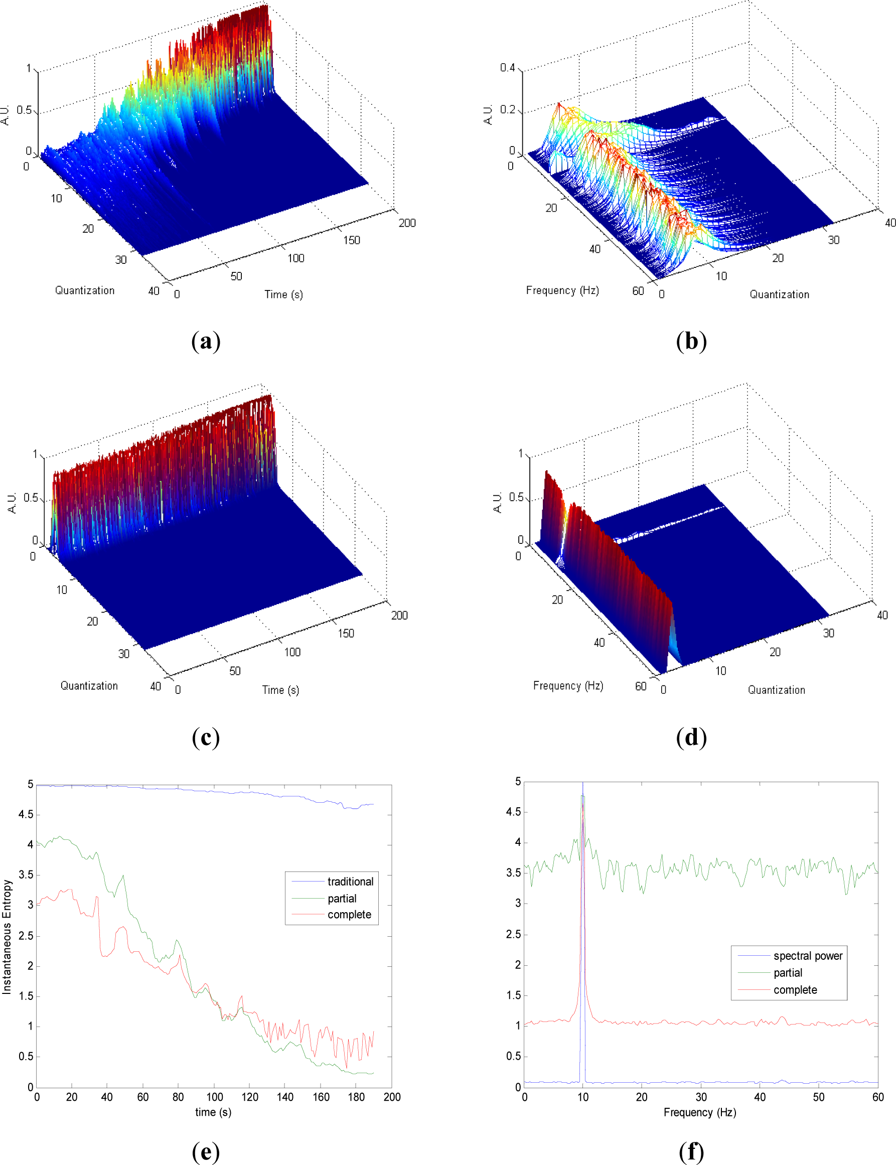
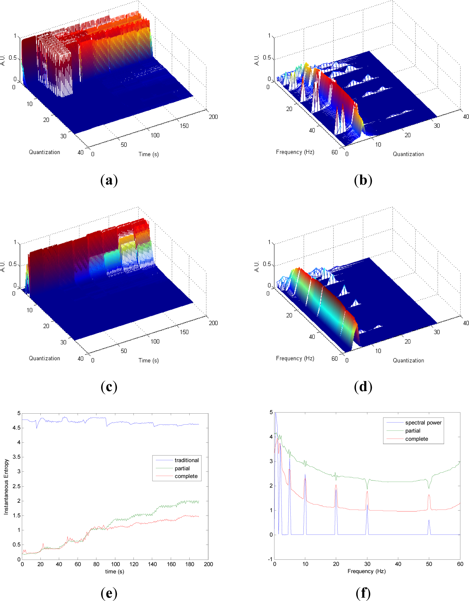
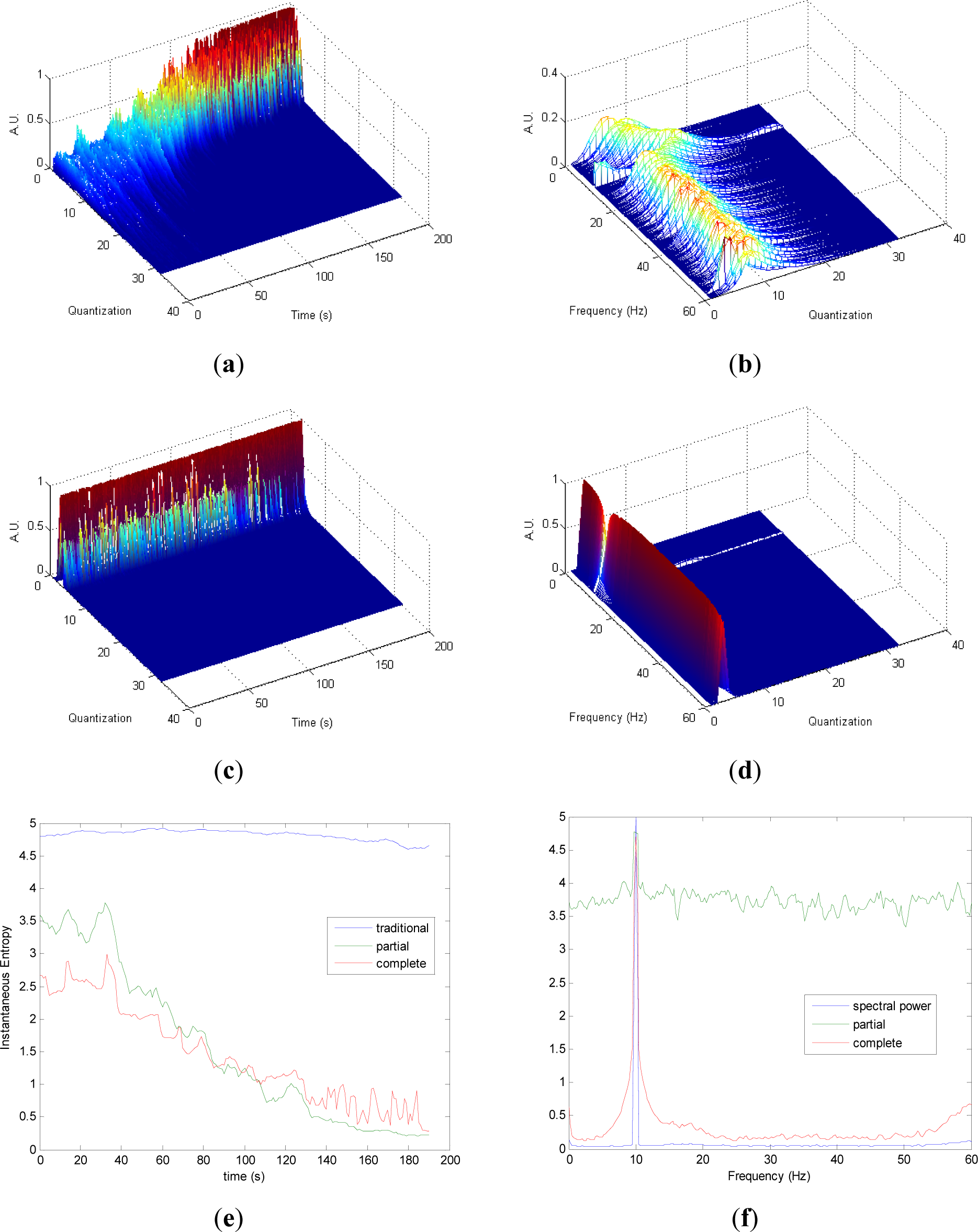
Figures 1 and 4 show the results obtained applying the methodology to all the synthetic signals.
Partial and complete distribution quantization vs. time of signal 1 are presented in Figures 1a,c, respectively. It can be observed that in cT all information is contained in few quantization bins, due to the fact that the quantization takes into account the complete CWD. On the contrary, since the quantization of pT takes into account separately the values of each time instant of CWD, the distribution of quantization-time is more homogeneous. Similar behavior is followed by pF and cF, as it is shown in Figures 1b,d, respectively. As it can be noted in Figure 1e, traditional Entr does not show significant changes when signal 1 evolves from one frequency component to the eight simultaneous frequency components, while pInstEntr and cInstEntr increase from one frequency component to the multiple components. However, pInstEntr has a higher increase than. cInstEntr In the frequency domain (Figure 1f), pSpInstEntr and cSpInstEntr have similar behavior to SpPow, showing the location of the frequency components f = Fi. However pSpInstEntr and cSpInstEntr decrease in low frequency until about 20 Hz and then they maintain stable values for f ≠ Fi. The higher values of pSpInstEntr and cSpInstEntr at low frequencies correspond to the persistent frequency components along the signal 1. The values of pSpInstEntr are above cSpInstEntr and approximately equidistant for all frequency values, except for the high frequency components (f = 30 Hz and f = 50 Hz) where pSpInstEntr and cSpInstEntr assume similar values.
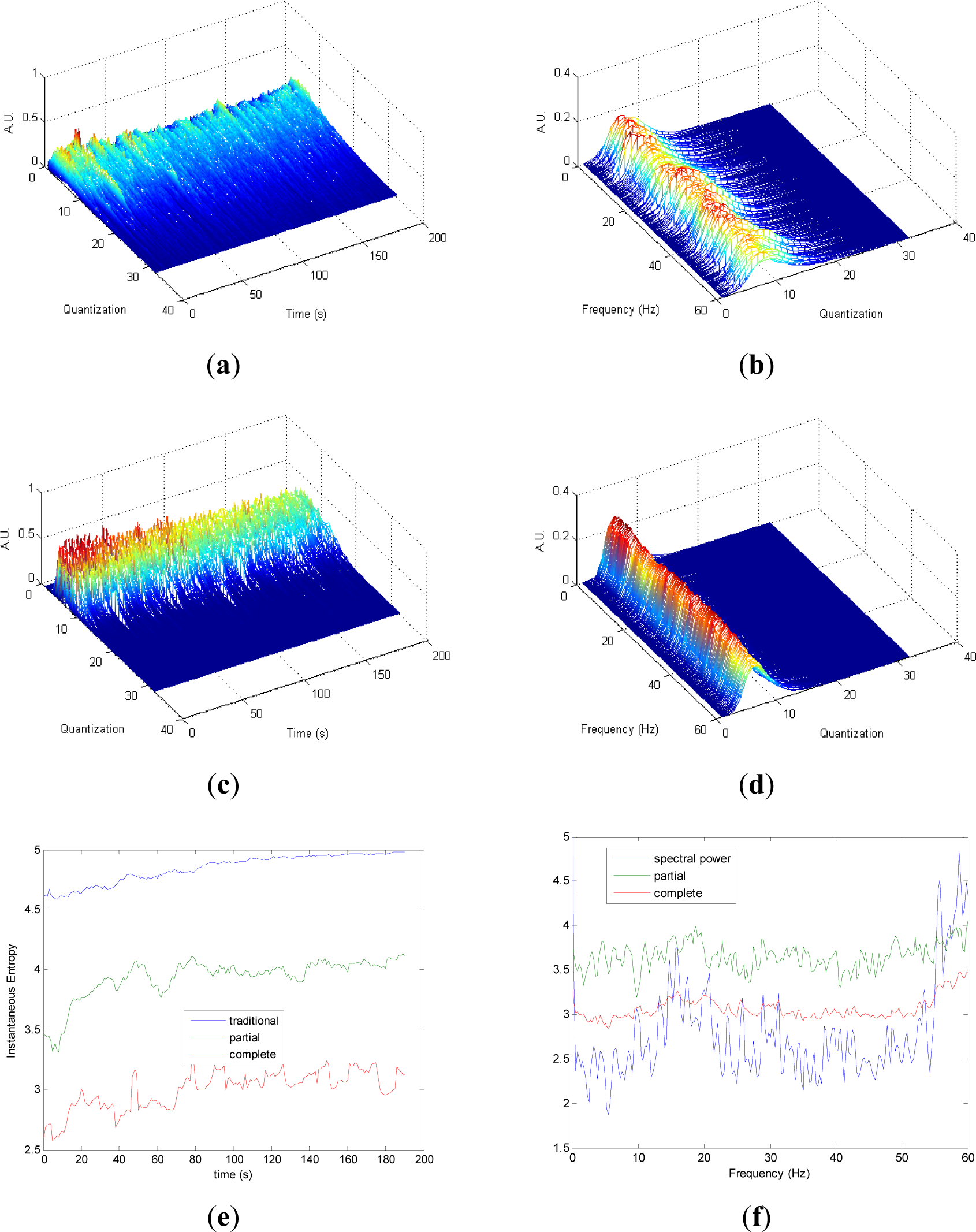
Partial and complete distributions quantization vs. time of signal 2 are presented in Figures 2a,c. During the transition from randomness to periodicity, the evolution of pT (Figure 2a) presents some changes that are less evident in cT (Figure 2c). The evolution of pT tends to be homogenous in the zone with more randomness. Observing quantization-frequency distributions in Figures 2b,d, all information is more contained in few quantization bins in cF than pF, due to the fact that the quantization takes into account the complete CWD in cF. In both pF and cF distributions, the oscillation frequency of the sinusoid is observed in 10 Hz. Traditional Entr (Figure 2e) does not show significant changes when the signal passes from a random to a periodic behavior. On the contrary, pInstEntr and cSpInstEntr decrease from randomness to periodicity. During random behavior pInstEntr is higher than cSpInstEntr then the two measures approach each other and converge in the zone with more periodicity. In Figure 2f, pSpInstEntr and cSpInstEntr show the location of the frequency component as SpPow does. While cSpInstEntr maintains stable values for the remaining frequencies, pSpInstEntr presents irregular oscillations in the entire spectrum. Values of pSpInstEntr are higher than cSpInstEntr except for the frequency component of the signal f = 10 Hz.
Similarly to the evolutions observed in Figure 2a,c, it can be noted in Figure 3a,c that the differences in the transition from chaos to periodicity in the evolution of pT (Figure 3a) are less evident in cT (Figure 2c). It is observed that less homogeneity behavior is preserved in pT in the zone with more chaos (Figure 3a) compared to the zone with more random (Figure 2a). Also, it can be noted that cT presents more heterogeneity along the time than in Figure 2c, due to the differences between chaos and random series. Quantization-frequency distributions of signal 3 (Figures 3b,d) have similar behavior to signal 2 (Figure 2b,d). Also Entr, pInstEntr, cInstEntr (Figure 3e), pSpInstEntr and cSpInstEntr (Figure 3f) exhibit similar behavior to signal 2. However, it can be noted when Figures 2f and 3f are compared that cSpInstEntr has a higher and a more constant base-line for all frequencies in signal 2 (Figure 2f) than in signal 3.
Quantization-time distributions of signal 4 are shown in Figure 4a,c. Certain differences are observed in the transition from chaos to randomness in the evolution of both pT and cT. The behavior of both distributions appear to be homogeneous. As it was observed in signals 1, 2 and 3, the information contained in quantization-frequency distributions of signal 4 (Figure 4b,d) is more concentrated in cF than pF. Then, since the complete distribution appears to be always more concentrated in few bins, it can be used when more resolution is required. Observing Figure 4e, Entr, pInstEntr and cInstEntr increase their values from chaos to random behavior of the signal. The entropy pInstEntr has higher values than cInstEntr for all the time instants. As it can be observed in Figure 4f, SpPow, pSpInstEntr and cSpInstEntr have similar behavior showing oscillations around three different constant baselines. Higher values are observed in pSpInstEntr than in cSpInstEntr.
Comparing the Figures 1e, 2e, 3e, and 4e, it can be deduced that when the signals contain many different frequency components, pInstEntr is higher than cInstEntr. This behavior is observed from approximately t = 100 s in Figure 1e, and till t = 60 s in Figures 2e and 3e. This is corroborated in Figure 4e where the analyzed signal combines chaos and random features along the time. However, when the signals have few frequency components, pInstEntr and cInstEntr have similar values. Comparing Figures 1f, 2f, 3f, and 4f, it is observed that both pSpInstEntrand cSpInfEntr tend to assume the same value where a frequency peak is present in the spectrum. For the remaining frequency components, pSpInfEntr has always higher values than cSpInfEntr.
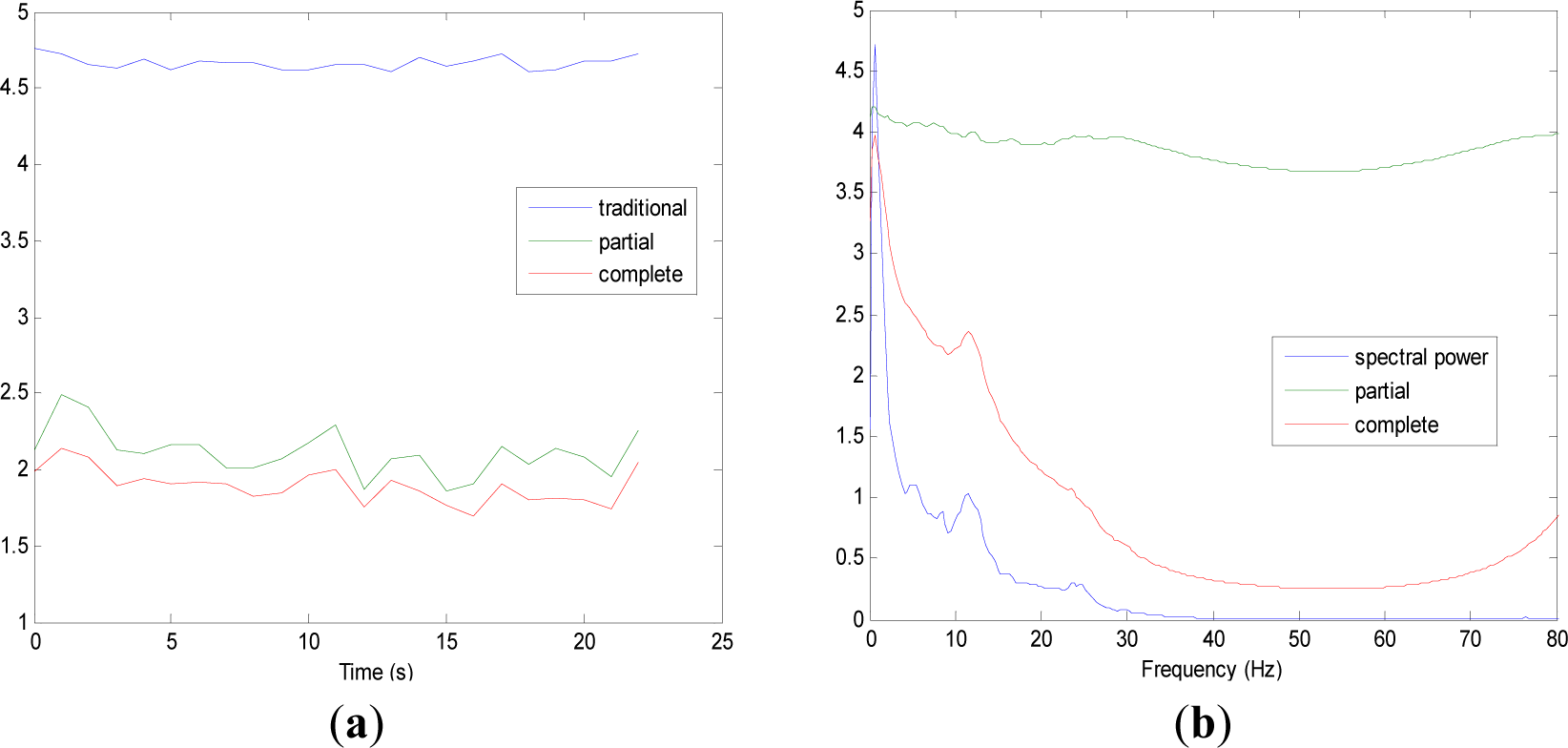
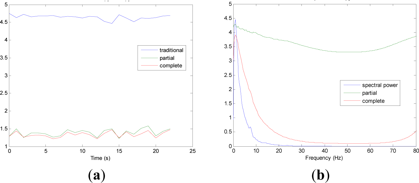
4.2. Real EEG Signals
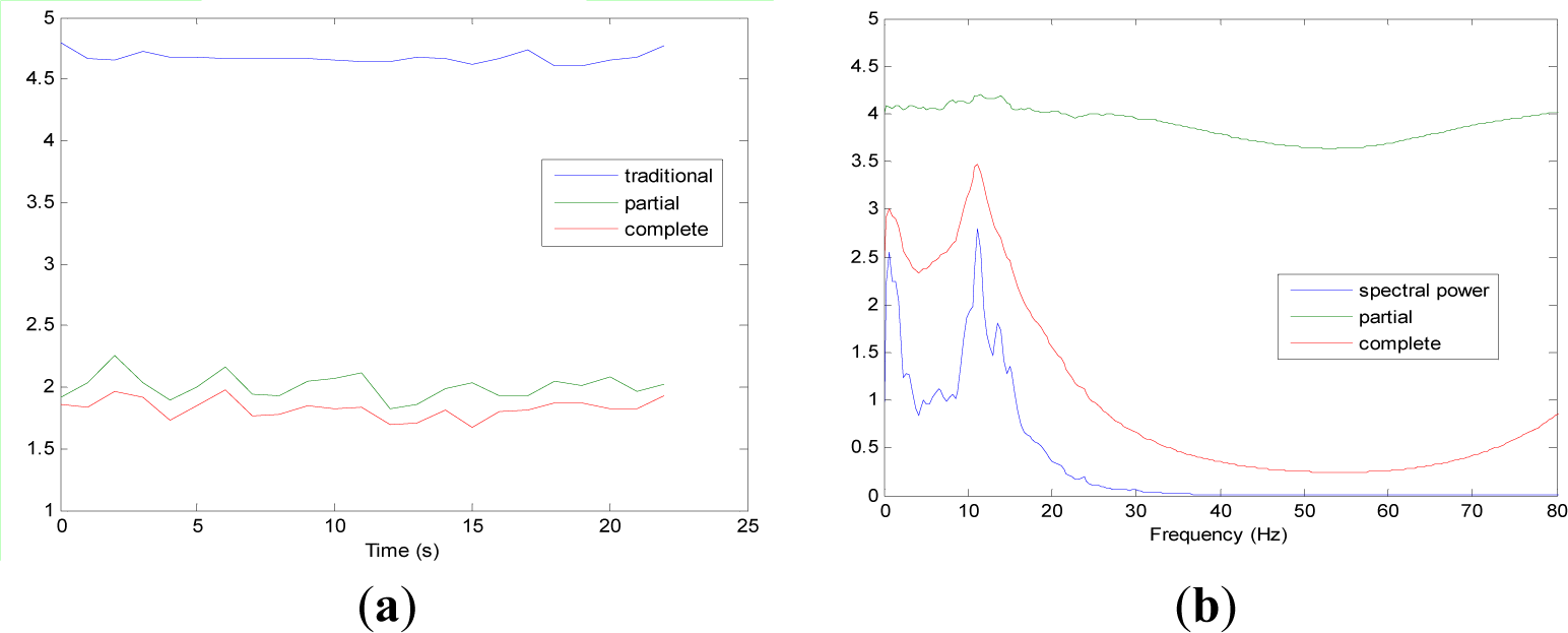
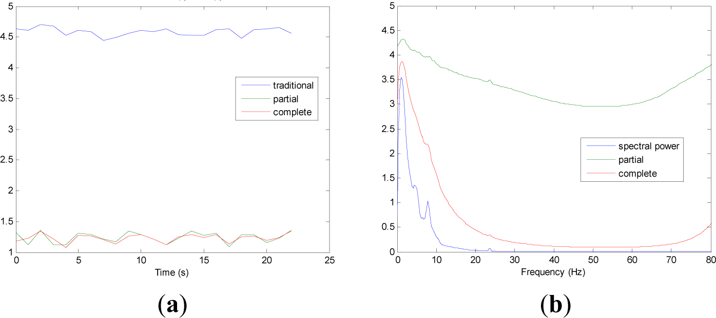
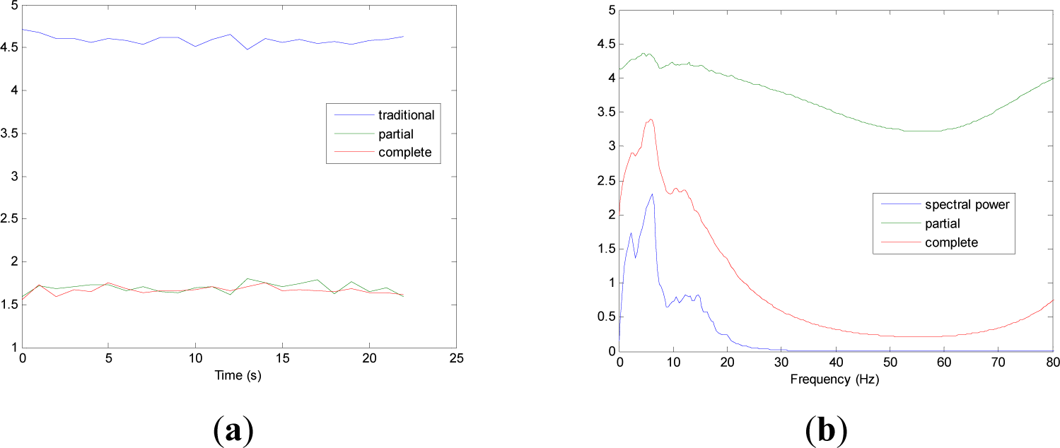
Figures 5 and 9 show the averaged evolution of cInstEntr, pInstEntr, Entr, cSpInfEntr, pSpInfEntr and SpPow of all EEG signals of each set. It can be observed that entropy pInstEntr has higher values than cInstEntr in set A and B for all time instants (Figures 5a and 6a, respectively), however, different behavior is seen in sets C, D and E (Figures 7a, 8a and 9a, respectively) where few slightly differences are observed between these two indexes. Traditional entropy Entr is always the highest. Observing Figures 5b, 6b, 7b, 8b and 9b, it can be noted that pSpInfEntr presents almost constant shape with higher values than cSpInfEntr for the entire frequency spectrum. On the contrary, the shape of cSpInfEntr is similar to SpPow, both presenting peaks in correspondence to certain frequency values. Entropies pSpInfEntr and cSpInfEntr tend to increase in high frequencies while the SpPow is zero.
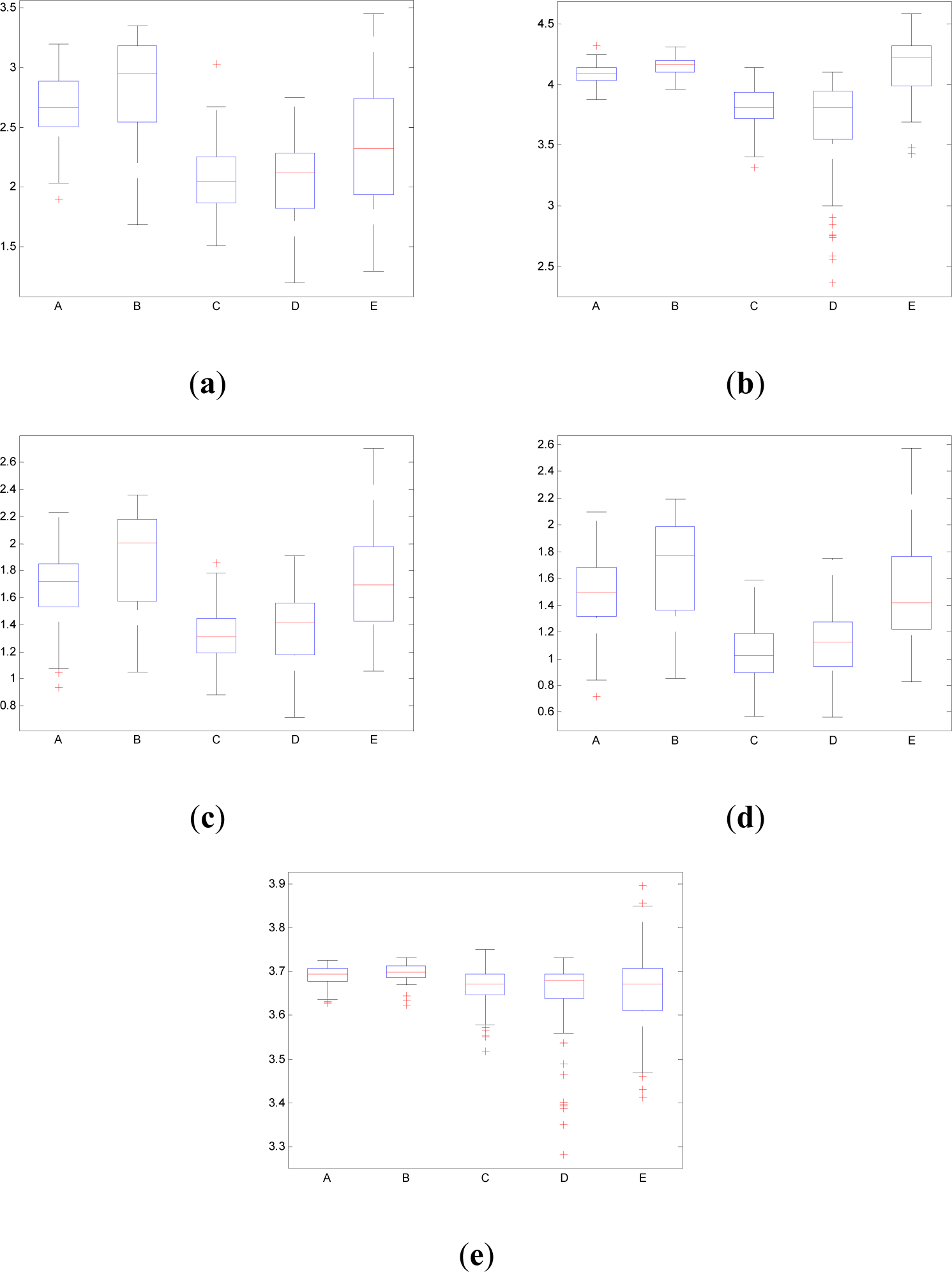
Figure 10 shows the boxplot of the mean values of pInstEntr, pSpInfEntr, cInstEntr, cSpInfEntr and Entr calculated for each EEG signal of each set (A,B,C,D,E). Table 1 contains the p-values (Mann-Whitney U-test) of the analyzed measures obtained by comparing sets: A vs. B, C vs. D, C vs. E and D vs. E.
The fundamental assumption of nonlinear techniques is that EEG signal is generated by nonlinear deterministic processes with nonlinear coupling interactions between neuronal populations. Nonlinearity in the brain is introduced, even at the neuronal level [13]. In recent years, with the application of the nonlinear dynamics to EEG, more evidences have indicated that the brain is a nonlinear dynamic system, and EEG signal can be regarded as its output [14]. In this way, it has been assumed that EEG signal is between random signal and deterministic signal [15].
As it can be seen in Figures 10c,d, higher values of cInstEntr and cSpInfEntr are related to eyes-closed state (set B) compared to eyes-open state (set A), with p-value = 0.0059 and p-value < 0.0005 (Table 1), respectively. Therefore, it can be inferred that the closing of eyes is associated with higher entropy in time and in frequency. Comparing these values with the evolution of the synthetic signals, higher entropy in time domain (cInstEntr) is associated with a predominance of random behavior respect to chaotic behavior and periodicity. Related to cSpInfEntr, the higher values of set B indicate a much more complexity behavior than in set A. It can be observed that cSpInfEntr of a random signal mixed with periodicity components (Figure 2f) contains a constant baseline with values higher than a chaotic signal mixed with periodicity components (Figure 3f). Therefore, it might be assumed that a random signal mixed with periodicity components has higher mean value of cSpInfEntr than a chaotic signal mixed with periodicity components. Then, cSpInfEntr of set A seems to have a behavior similar to chaos mixed with periodicity (shown in Figure 3f) and cSpInfEntr of set B seems to have a behavior similar to random mixed with periodicity (shown in Figure 2f).
Regarding the sets C, D and E of the EEG database, there are very significant differences between the values of pInstEntr, pSpInfEntr, cInstEntr, cSpInfEntr computed for non-ictal (sets C and D) and ictal (set E) states, with p-value < 0.0005 (Table 1). In this case, the higher value of these measures in ictal activity is associated with more complex behavior in time-frequency domain. Since the literature [16] is almost concordance to the fact that epileptic seizure is associated with a decrease of complexity of the EEG signal in time domain, we assume that higher values of pInstEntr, pSpInfEntr, cInstEntr, cSpInfEntr in set E seem to indicate a higher complexity in frequency domain.
Certain differences are observed between the inter-ictal activity recorded from the epilogenetic zone (set C) and from the opposite brain hemisphere (set D) in the frequency domain (pSpInfEntr and cSpInfEntr in Figures 10(b,d), respectively), with p-value < 0.05. However, there are not statistical differences between the inter-ictal activity recorded from the epilogenetic zone (set C) and from the opposite brain hemisphere (set D) in the time domain (pInstEntr and cInstEntr in Figures 10(a,c), respectively).
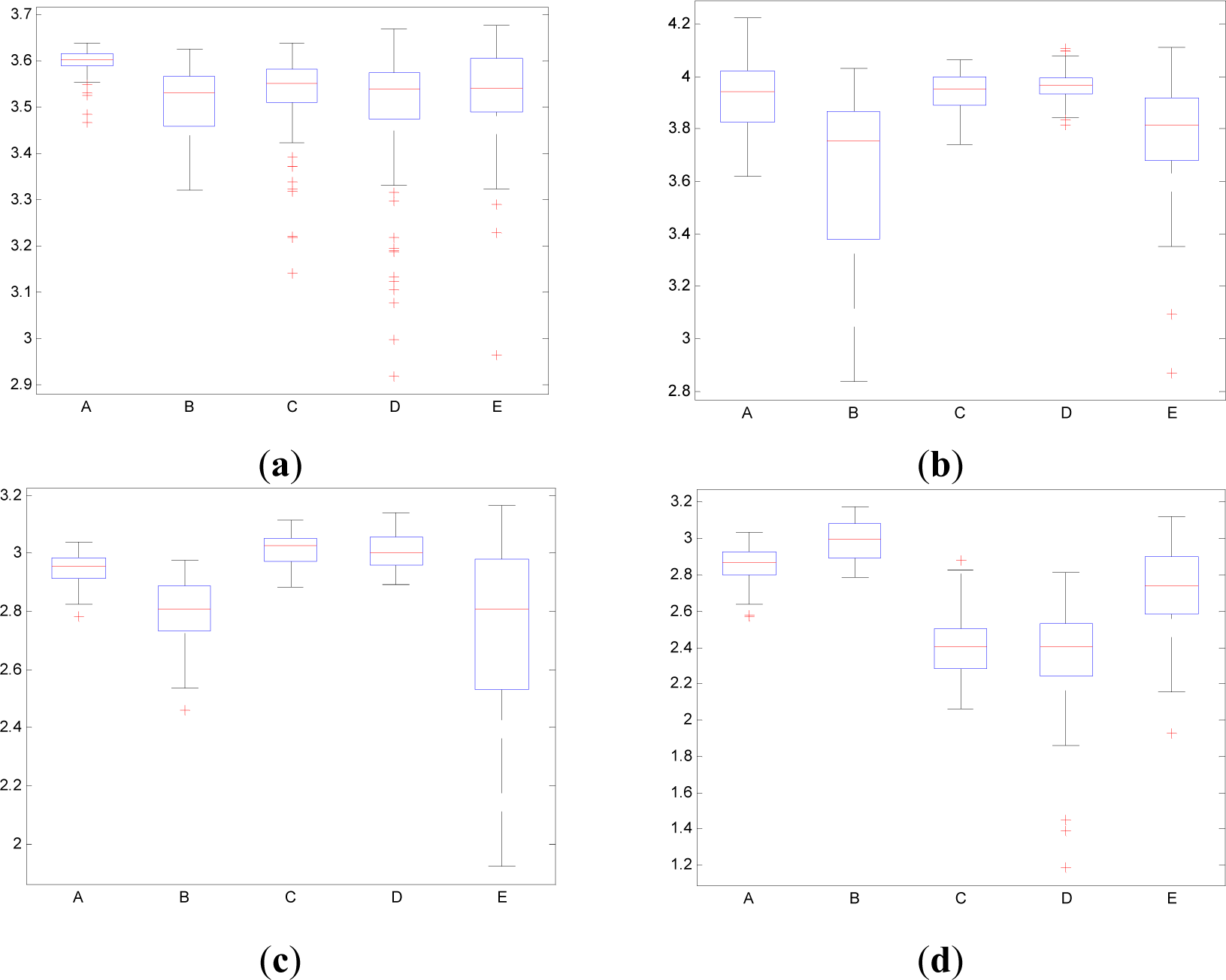
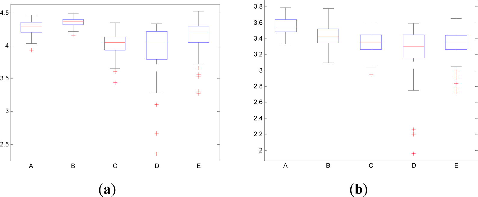
In contrast to the traditional time domain information measures as the Entr, the CWD permits to divide the spectrum in order to isolate specific frequency bands. This property permits to calculate the pInstEntr, pSpInfEntr, cInstEntr, cSpInfEntr in the traditional frequency bands of the EEG signal (delta, theta, alpha, beta, gamma). Figures 11 and 12 show the boxplot of the distributions of the pInstEntr, pSpInfEntr, cInstEntr, cSpInfEntr calculated in the frequency bands that give the best statistical significant results. The statistical significance levels are presented in Table 2.
It is well known that the closed eyes condition produces certain changes in the EEG. One of the most remarkable alterations is the rise in the power of the alpha rhythm [13]. Thus, the EEG spectrum is modified in comparison to the eyes-open case. These modifications have been also detected by the instantaneous and spectral information entropy measures depicted in Figures 11 and 12.
As it can be seen in Figure 11a–c, lower values of pInstEntr in alpha and beta, and cInstEntr in delta are related to the eyes-closed state (set B) compared to eyes-open state (set A), with p-value < 0.0005. On the contrary, cInstEntr assumes higher values in set B than set A with p-value < 0.0005 when alpha band is studied. Therefore, it can be inferred that the closing of eyes causes transference of information between delta and alpha frequency bands. In addition, the boxplots depicted in Figure 11a,d show differences between sets A and B, pInstEntr values decrease from set A to set B while cInstEntr values increase. Since the value obtained considering independently each time instant (partial distribution pT) has different behavior from the value obtained considering all time instants (total distribution cT) we assume that the information provided by the alpha rhythm presents non-stationary behavior. Regarding the subsets C, D and E of the EEG database, there are very significant differences between non-ictal (sets C and D) and ictal (set E) states, due to the values of pInstEntr in beta (Figure 11b), cInstEntr in delta (Figure 11c) and in alpha frequency bands (Figure 11d), with p-value < 0.0005. In this case, higher values of pInstEntr in beta (Figure 11b) and in delta band (Figure 11c) are observed in non-ictal activity (sets C and D) while cInstEntr has a reverse behavior (Figure 11d).
Higher values of pSpInfEntr in beta band (Figure 12a) are related to the eyes-closed state (set B) compared to eyes-open state (set A), with p-value < 0.0005. Contrarily, cSpInfEntr (Figure 12(b)) assumes lower values in set B than in set A with p-value < 0.0005 when beta band is studied. This behavior indicates a high contain of power in beta band for eyes-open state (set A) compared with eyes-closed state (set B), as it is observed in cSpInfEntr (Figure 12b). Contrarily, high values of pSpInfEntr in eyes-closed state indicate that the beta rhythm is more regularly present along the time of the EEG recording. These different behaviors are observed in synthetic signal 1 in which the low frequencies are present in all the evolution of the simulated signal (Figure 1f). Regarding the subsets C, D and E of the EEG database, there are very significant differences (p-value < 0.0005) between non-ictal (sets C and D) versus ictal (set E) states, however only for the values of pSpInfEntr in beta band (Figure 12a). In this case, higher values of pSpInfEntr in beta (Figure 12a) are observed in ictal activity (set E).
Table 3 shows the sensitivity (Sen) and specificity (Spe) calculated with the leaving-one-out method and the area under the ROC curve (AUC) of the best measures obtained by comparing EEG sets. It can be noted that measures of pInstEntr, cInstEntr and SpInfEntr permitted to obtain Sen > 65%, Spe > 70% and AUC > 0.75 in the discrimination between A and B sets. Furthermore, measures of pInstEntr and cInstEntr yield Sen > 75%, Spe > 80% and AUC > 0.8 in the discrimination between C, D and E sets.
5. Conclusions
A new approach to calculate TFR entropy has been presented and applied to simulated and real physiological time series. This approach is based on the definition of Shannon entropy applied to the probability mass function of the TFR in both time and frequency domain. In this way, the smoothing inherent in the calculation of the entropy is avoided and instantaneous values of this measure are obtained.
This methodology takes advantage of the property inherent to TFR that permits to deal with non-stationary signals together with the property of Shannon entropy that deals with chaoticity, complexity and randomness.
The results have shown that the values of the proposed measures tend to decrease, with different proportion, when the behaviors of the synthetic signals evolve from chaos or randomness to periodicity. Finally, this paper has demonstrated that they can be useful tools to quantify the different periodic, chaotic and random components in EEG signals.
Acknowledgments
This work was supported within the framework of the CICYT grant TEC2010-20886 from the Spanish Government and the Research Fellowship Grant FPU AP2009-0858 from the Spanish Government. CIBER of Bioengineering, Biomaterials and Nanomedicine is an initiative of ISCIII.
Author Contributions
All authors collaborated and contributed extensively to the work presented in this paper. More specifically: Umberto Melia, Francesc Claria and Montserrat Vallverdu designed the methodology and wrote the paper; Umberto Melia carried out the development of the algorithms and the application of the entropy measures to real and simulated signals; Pere Caminal had the general overview of the work.
Conflicts of interest
The authors have declared no conflicts of interest.
References
- Kotelnikov, V.A. On the carrying capacity of the ether and wire in telecommunications, In Proceedoings of the First All-Union Conference on Questions of Communication, Izd. Red. Upr. Svyazi RKKA, Moscow, Russia; 1933.
- Shannon, C.E. Communication in the presence of noise. Proc. Inst. Radio Eng 1949, 37, 10–21, Reprint in: Proc. IEEE 1998, 86, 2. [Google Scholar]
- Cohen, L. Time-Frequency Analysis; Prentice Hall Signal Processing Series; Prentice Hall: Englewood Cliffs, NJ, USA, 1995. [Google Scholar]
- Flandrin, P. Time-Frequency and Time-Scale Analysis; Academic: San Diego, CA, USA, 1999. [Google Scholar]
- Williams, W.J.; Brown, M.L.; Hero, A.O. Uncertainty, information, and time-frequency distributions. Proc. SPIE Int. Soc. Opt. Eng 1991, 1566, 144–156. [Google Scholar]
- Baraniuk, R.G. Measuring Time–frequency information content using the Rényi entropies. IEEE Trans. Inf. Theor 2001, 47, 1391–1409. [Google Scholar]
- Jeong, J. EEG dynamics in patients with Alzheimer’s disease. Clin. Neurophysiol 2004, 115, 1490–1505. [Google Scholar]
- Clariá, F.; Vallverdú, M.; Riba, J.; Romero, S.; Barbanoj, M.J.; Caminal, P. Characterization of the cerebral activity by timefrequency representation of evoked EEG potentials. Physiol. Meas 2011, 32, 1327–1346. [Google Scholar]
- Pincus, S.M. Approximate entropy as a measure of system complexity. Proc. Natl. Acad. Sci. USA 1991, 88, 2297–2301. [Google Scholar]
- Ferrario, M.; Signorini, M.G.; Magines, G.; Cerutti, S. Comparison of entropy-based regularity estimators: Application to the fetal heart rate signal for the identification of fetal distress. IEEE Trans. Biomed. Eng 2006, 53, 119–125. [Google Scholar]
- Escudero, J.; Hornero, R.; Abasolo, D. Interpretation of the auto-mutual information rate of decrease in the context of biomedical signal analysis. Application to electroencephalogram recordings. Physiol. Meas 2009, 30, 187–199. [Google Scholar]
- Davies, B. Exploring Chaos theory And Experiment; Perseus Books: Reading, MA, USA, 1999. [Google Scholar]
- Andrzejak, R.G.; Lehnertz, K.; Moormann, F.; Rieke, C.; David, P.; Elger, C.E. Indications of nonlinear deterministic and finite-dimensional structures in time series of brain electrical activity: Dependence on recording region and brain state. Phys. Rev 2001, 64, 061907. [Google Scholar]
- Korn, H.; Faure, P. Is there chaos in the brain? II. Experimental evidence and related models. Comptes Rendus Biol 2003, 326, 787–840. [Google Scholar]
- Wang, X.; Meng, J.; Tan, G.; Zou, L. Research on the relation of EEG signal chaos characteristics with high-level intelligence activity of human brain. Nonlinear Biomed. Phys 2010, 4, 2. [Google Scholar]
- Babloyantz, A.; Destexhe, A. Low-dimensional chaos in an instance of epilepsy. Proc. Natl. Acad. Sci. USA 1986, 83, 3513–3517. [Google Scholar]


| Sets | pInstEntr | pSpInfEntr | cInstEntr | cSpInfEntr |
|---|---|---|---|---|
| A vs. B | 0.2360n.s. | 0.1547n.s. | 0.0059 | 0.00003 |
| C vs. D | 0.9861n.s. | 0.0147 | 0.1096n.s. | 0.0399 |
| C vs. E | <0.0005 | <0.0005 | <0.0005 | <0.0005 |
| D vs. E | <0.0005 | <0.0005 | <0.0005 | <0.0005 |
n.s., non-statistical significant.
| Sets | pInstEntr | cInstEntr | pSpInfEntr | cSpInfEntr | ||
|---|---|---|---|---|---|---|
| alfa band | beta band | delta band | alfa band | beta band | beta band | |
| A vs. B | <0.0005 | <0.0005 | <0.0005 | <0.0005 | <0.0005 | <0.0005 |
| C vs. D | 0.0706n.s. | 0.0467 | 0.2328n.s. | 0.9013n.s. | 0.8214n.s. | 0.0235 |
| C vs. E | 0.9151n.s. | <0.0005 | <0.0005 | <0.0005 | <0.0005 | 0.9249n.s. |
| D vs. E | 0.1284n.s. | <0.0005 | <0.0005 | <0.0005 | <0.0005 | 0.0341 |
n.s., non-statistical significant.
| Sets | Measure | Sen | Spe | AUC |
|---|---|---|---|---|
| A vs. B | pInstEntr (alfa) | 69.0 | 90.3 | 0.896 |
| cInstEntr (delta) | 67.6 | 90.3 | 0.905 | |
| cSpInfEntr(beta) | 66.2 | 72.2 | 0.784 | |
| C vs. E | cInstEntr | 76.8 | 82.8 | 0.881 |
| cInstEntr (alfa) | 77.8 | 82.8 | 0.874 | |
| cInstEntr (beta) | 73.7 | 63.6 | 0.758 | |
| D vs. E | cInstEntr | 83.8 | 75.8 | 0.893 |
| pInstEntr (beta) | 61.6 | 96.0 | 0.853 |
© 2014 by the authors; licensee MDPI, Basel, Switzerland This article is an open access article distributed under the terms and conditions of the Creative Commons Attribution license (http://creativecommons.org/licenses/by/3.0/).
Share and Cite
Melia, U.; Claria, F.; Vallverdu, M.; Caminal, P. Measuring Instantaneous and Spectral Information Entropies by Shannon Entropy of Choi-Williams Distribution in the Context of Electroencephalography. Entropy 2014, 16, 2530-2548. https://doi.org/10.3390/e16052530
Melia U, Claria F, Vallverdu M, Caminal P. Measuring Instantaneous and Spectral Information Entropies by Shannon Entropy of Choi-Williams Distribution in the Context of Electroencephalography. Entropy. 2014; 16(5):2530-2548. https://doi.org/10.3390/e16052530
Chicago/Turabian StyleMelia, Umberto, Francesc Claria, Montserrat Vallverdu, and Pere Caminal. 2014. "Measuring Instantaneous and Spectral Information Entropies by Shannon Entropy of Choi-Williams Distribution in the Context of Electroencephalography" Entropy 16, no. 5: 2530-2548. https://doi.org/10.3390/e16052530