The Impact of the Prior Density on a Minimum Relative Entropy Density: A Case Study with SPX Option Data

Abstract

We study the problem of finding probability densities that match given European call option prices. To allow prior information about such a density to be taken into account, we generalise the algorithm presented in Neri and Schneider (Appl. Math. Finance 2013) to find the maximum entropy density of an asset price to the relative entropy case. This is applied to study the impact of the choice of prior density in two market scenarios. In the first scenario, call option prices are prescribed at only a small number of strikes, and we see that the choice of prior, or indeed its omission, yields notably different densities. The second scenario is given by CBOE option price data for S&P500 index options at a large number of strikes. Prior information is now considered to be given by calibrated Heston, Schöbel–Zhu or Variance Gamma models. We find that the resulting digital option prices are essentially the same as those given by the (non-relative) Buchen–Kelly density itself. In other words, in a sufficiently liquid market, the influence of the prior density seems to vanish almost completely. Finally, we study variance swaps and derive a simple formula relating the fair variance swap rate to entropy. Then we show, again, that the prior loses its influence on the fair variance swap rate as the number of strikes increases.

1. Introduction

Many financial derivatives are valued by calculating their expected payoff under the risk-neutral measure. For path-independent derivatives, the expectation can be obtained by integrating the product of the payoff function and the density.

If a pricing model has been chosen for a market in which many derivative products are actively quoted, then often, due to the limited number of model parameters, this model will be unable to perfectly match the market quotes, and a compromise must be made during model calibration by using some kind of “best-fit” criterion.

If no model has been chosen, one can try to imply from the market data for a given maturity a probability density function that leads, by integration as described above, exactly back to the quoted prices. However, unless the market is perfectly liquid, there will be infinitely many densities that match the price quotes, and some criterion for the selection of the density will have to be applied. One such criterion is to choose the density that maximises uncertainty or, in another word, entropy. The idea is that between two densities matching the constraints imposed by the market prices, the one that is more uncertain—where “uncertain” means, very roughly speaking, spreading probability over a large interval instead of assigning it to just a few points, where possible—should be chosen. In general, applying the criterion of entropy delivers convincing results. For example, on the unit interval [0,1], if no constraints are given, the density with the greatest entropy—the maximum entropy density (MED)—is the uniform density. On the positive real numbers [0, ∞), if the mean is given as the only constraint, the entropy maximiser is the exponential density. There is no entropy maximiser over the real numbers ℝ, but if the mean and variance are imposed as constraints, then the density with largest entropy is a normal density.

A third approach, which we will use to combine the two approaches described above, is to take a density p, which may be near to matching some imposed constraints, as a prior density and to then find a density q that is “as close” as possible to p and exactly matches these constraints. The criterion we will employ to measure the “distance” between the densities q and p is that of relative entropy. Since we are trying to depart as little as possible from the prior p, our goal will be to find the minimum relative entropy density (MRED) q that matches the given constraints. Of course, if the prior p already matches the constraints, then we can take as our solution q = p, since the relative entropy of p with respect to itself is zero.

The concept of entropy has its origins in the works of Boltzmann [1] in Statistical Mechanics and Shannon [2] in Information Theory. Relative entropy was introduced by Kullback and Leibler [3] and is also known as the Kullback-Leibler information number I = I(q||p) or I-Divergence [4]. To see applications of relative entropy to a wide range of areas such as combinatorial optimisation, simulation or machine learning, readers are referred to the book by Rubinstein and Kroese [5].

In Finance, too, entropy has become a popular tool. Buchen and Kelly [6] and Stutzer [7] (see also [8–10]) were the first to apply the optimisation of entropy and relative entropy to the estimation of the distribution of an underlying asset from given option prices. As a prior density in the relative entropy approach, Buchen and Kelly take a Black–Scholes log-normal density, whereas Stutzer uses historical returns to obtain a discrete density. As Buchen and Kelly, and in contrast to Stutzer, we consider the continuous case. However, we consider densities coming from a larger class of models.

Borwein et al. [11] analyse the non-relative Buchen–Kelly approach in the framework of partially finite convex programming, legitimise the formal calculations involving Lagrange multipliers, and provide an analysis of the constraints. In a brief conclusion, they remark on how their analysis can be extended to the case when a given density is taken as prior information.

Orozco Rodriguez and Santosa [12] analyse the stability of the algorithm presented in [11]. Since an explicit dual function only exists in the non-relative case, they restrict their analysis to maximisation of Boltzmann–Shannon entropy. They also point out the instability of the Buchen–Kelly algorithm. We tried their examples with the algorithm introduced by Neri and Schneider [13] and experienced no instability issues. In the present work, we generalise the algorithm of [13] to the relative entropy case.

Frittelli [14] studies the existence of the minimal entropy martingale measure (MEMM) in an incomplete market and relates its density to exponential utility functions. Fujiwara and Miyahara [15] study the existence and form of the MEMM in the context of geometric Lévy processes and obtain results relating the MEMM price of a contingent claim to its utility indifference price for an exponential utility function. In both cases, the MEMM is minimal in the sense of the relative entropy distance to a given prior measure.

Avellaneda et al. [16] present an algorithm to calibrate a volatility surface to option prices quoted in the market, which is based on minimising the relative entropy distance of an arbitrage-free diffusion process to a prior diffusion.

Gulko [17–19] develops a framework based on entropy maximisation and derives models to price stock and bond options. Brody et al. [20,21] use entropy maximisation to obtain option pricing formulas and focus on option Greeks, and in particular on option gamma. In [22], they consider the maximisation of Rényi entropy to obtain power-law densities instead of piece-wise exponential densities. The choice of the parameter defining the Rényi entropy gives an extra degree of freedom, which allows to control the tails of the density. However, they do not consider prior densities and relative entropy minimisation.

Surveys of applications of entropy in finance are given by Hawkins [23] and, more recently, Zhou, Cai and Tong [24].

In the study we carry out in this paper, the prior density function of the asset price for a fixed maturity is given by a model, such as the Black–Scholes model or the Heston stochastic volatility model. Depending on the model in question, this prior density will be either directly available in analytical form (in the case of the Black–Scholes model a log-normal distribution), or have to be obtained numerically (in case of the Heston model via Fourier inversion). The algorithms we propose to calculate the MRED q (with respect to p) satisfying some constraints given by European option prices are extensions of the two algorithms presented in [13,25].

In the first case, the option data consists of call and digital call prices (Section 3), and in the second case only of call prices (Section 4). If only the call prices are imposed, say n of them, the problem consists in finding the minimum of a real-valued, convex function (the relative entropy function) in n variables. If one additionally imposes the n prices of digital options at the same strikes, the problem simplifies to a sequence of n one-dimensional root-finding problems. The multi-dimensional algorithm makes use of the single-dimensional one by fixing the set of call prices, defining a parameter space Ω for arbitrage-free digital prices, and then finding the unique density in this family with the smallest relative entropy.

The models we take to generate our prior densities are presented in Section 5, together with a review of the characteristic function pricing approach and the corresponding Fourier transform techniques. In addition to the two models already mentioned above, we also consider the Schöbel-Zhu stochastic volatility model and the Variance Gamma model.

In Section 6 we study two market scenarios. In the first one, we take a log-normal Black-Scholes and a Heston density as our priors and calculate the MREDs that match given call prices. We then compare option prices to those obtained with an MED, and also to those obtained with another log-normal density that matches the constraints, and observe that the price differences can be substantial. In the second scenario, we take S&P500 call option prices from the CBOE. This market is very liquid, and for the maturity we consider we have quotes for a large set of strikes. We calibrate a Heston model, a Schöbel-Zhu model and a Variance Gamma model to this data and use the densities generated by these models as prior densities. Then, we calculate the three MREDs for these priors, and compare the digital option prices they give to those given by the original models, those given by an MED, and finally the market prices themselves, which are available in this case. We observe that it makes almost no difference which model is chosen for the prior, and that all three MREDs essentially agree with the MED.

In Section 7 we study variance swaps and the fair swap rate. Assuming that the underlying asset follows a diffusion process without jumps, it is possible to relate this rate to the price of a log-contract. A formula linking it to an integral over call and put prices at varying strikes is also well known ([26–28]). Here, we establish a simple formula (Corollary 2) that relates the fair variance swap rate to entropy. We then give an explicit formula (see Equation (38)) for the fair variance swap rate in the case of a (non-relative) MED in terms of the assumed drift rate and the density’s parameters. In the relative entropy case, we calculate the fair rate numerically and show that for MREDs constrained by data at very few strikes the prior density can have a significant impact on the fair rate. However, as in the examples given in Section 6, the impact of the prior density diminishes rapidly as data at more strikes are added as constraints. Finally, Section 8 concludes the article.

2. Relative Entropy and Option Prices

In this section we review the concept of relative entropy, which can be regarded as a way of measuring the “distance” between two given densities. Our goal is to apply this measure to the following problem: Given a prior density p, coming for example from a model that fits well, but not exactly, European option prices observed in the market, how can we deform this density in such a way that it exactly matches these prices but stays as close as possible to the original density under the criterion of relative entropy?

2.1. Relative Entropy

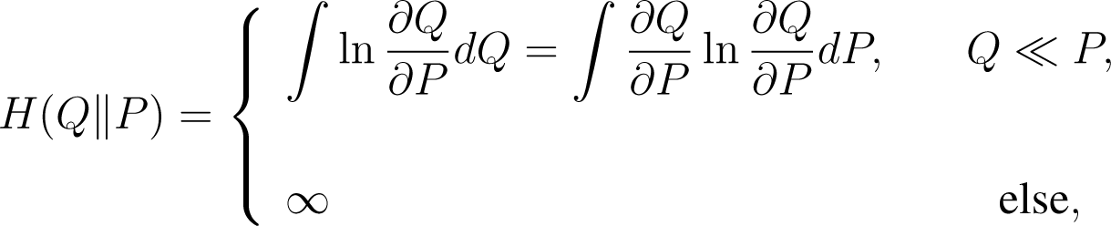
For two probability distributions Q and P, the relative entropy of Q with respect to P is defined by

(1)

where ∂Q/∂P is the Radon–Nikodým derivative. From the inequality S ln S ≥ S − 1 we have

We also have H(Q||P) = 0 if, and only if, Q = P. However, relative entropy is not a metric since, in general, H(Q||P) ≠ H(P||Q), and the triangle inequality is not satisfied either. Even the symmetric function H(Q||P) + H(P||Q) does not define a metric, since it still does not satisfy the triangle inequality [29].

The Csiszár–Kullback inequality [30,31] relates relative entropy to distance between densities in the sense of the L¹(0, ∞) norm:

$${\Vert q-p\Vert }_{L^1}:={\displaystyle {\int }_0^{\infty }\left|q(S)-p(S)\right|dS\le \sqrt{2H(q||p)}},$$

where

$$H(q||p)={\displaystyle \int q(S)\ln \frac{q(S)}{p(S)}dS}={\displaystyle \int \frac{q(S)}{pS)}\ln \frac{q(S)}{p(S)}p(S)dS}$$

(2)

is the same definition as Equation (1) above in terms of densities, which means in particular that convergence in the sense of relative entropy implies L¹-convergence.

2.2. Minimiser Matching Option Prices

We now give a precise formulation of the minimisation problems that we want to solve. Let p be the prior density on [0, ∞), which is assumed to be strictly positive almost everywhere.

For a fixed underlying asset and maturity T, we are given undiscounted prices ${\tilde{C}}_1,\dots ,{\tilde{C}}_n$ of call options at strictly increasing strikes $K_1<\cdots <K_n$. For notational convenience, we introduce the “strikes” K₀:= 0 and K_n+1 := ∞ and make the convention that ${\tilde{C}}_0$ is the forward asset price for time T and ${\tilde{C}}_{n+1}=0$.

In Section 4 we will determine a density q for the underlying asset price S(T) at maturity that minimises relative entropy H(q||p) under the constraints

$${\mathbb{E}}^q[{(S(T)-K_i)}^{+}]={\tilde{C}}_i,i.e.,{\displaystyle {\int }_{K_i}^{\infty }(S-K_i)q(S)dS=}{\tilde{C}}_i\forall i=0,\dots ,n.$$

(3)

Before that, in Section 3, we shall assume that undiscounted digital option prices ${\tilde{D}}_1,\dots ,{\tilde{D}}_n$ on the same asset, maturity and strikes are also given and we look for q that, in addition, verifies the constraints

$${\mathbb{E}}^q[{\mathbf{I}}_{\{S(T)>K_i\}}]={\tilde{D}}_i\text{,}i.e.,{\displaystyle {\int }_{K_i}^{\infty }q(S)dS={\tilde{D}}_i\forall i=0,\dots ,n}.$$

(4)

Again, for ease of notation, we make the convention that ${\tilde{D}}_0=1$ and ${\tilde{D}}_{n+1}=K_{n+1}{\tilde{D}}_{n+1}=0$. Notice that the constraints Equations (3) and (4) for i = 0 are consistent with the fact that q is a density (its integral is 1) and the martingale condition

$${\mathbb{E}}^q\left[S(T)\right]={\displaystyle {\int }_0^{\infty }Sq}(S)dS={\tilde{C}}_0.$$

3. Minimiser Matching Call and Digital Option Prices

In this section we review some results stated in [25] and provide the base arguments required to prove them in case a prior density p is given and call and digital options prices are prescribed.

In addition, we show how the algorithm presented in [25] can be efficiently implemented. We do not assume that p is given analytically, and therefore the implementation requires numerical integration. However, the availability of the digital prices allows for an efficient solution locally in each “bucket”, i.e., interval [K_i, K_i+1), via a one-dimensional Newton–Raphson rootfinder.

Formally applying the Lagrange multipliers theorem, as in [6], it can be “proven” (rigorously speaking, the Lagrange multipliers theorem cannot be applied since the relative entropy functional is nowhere continuous [11]) that if q minimises relative entropy in respect to p, then the Radon-Nikodým derivative g := ∂Q/∂P = q/p is piecewise exponential. More precisely, on each interval [K_i, K_i+1) the density q is given by

$$q(S)=g(S)p(S)={\alpha }_i{e}^{{\beta }_{i}S}p(S),$$

(5)

where α_i,β_i ∈ ℝ, α_i > 0 are parameters that still have to be determined using the following two constraints imposed by the option data, which are an equivalent reformulation of the constraints Equations (3) and (4) given above, but allow for an easy solution.

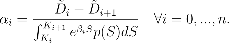
The first constraint follows directly from Equation (4) and is given by

$$\begin{array}{cc}{\alpha }_i{\displaystyle {\int }_{K_i}^{K_{i+1}}{e}^{{\beta }_{i}S}p(S)dS={\tilde{D}}_i-}{\tilde{D}}_{i+1},& \forall i=0,\dots ,n.\end{array}$$

from which we have

(6)

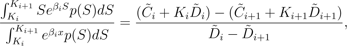
The second constraint also follows directly from Equations (3) and (4) and is given by

$${\alpha }_i\begin{array}{cc}{\displaystyle {\int }_{K_i}^{K_{i+1}}S{e}^{{\beta }_{i}S}p(S)dS=({\tilde{C}}_i+K_i{\tilde{D}}_i)-({\tilde{C}}_{i+1}+K_{i+1}{\tilde{D}}_{i+1}),}& \forall i=0,\dots ,n.\end{array}$$

Notice that the right hand side of the equation above is the undiscounted price of an “asset-or-nothing” derivative that pays the asset price itself if it finishes between the two strikes K_i and K_i+1 at maturity and zero otherwise. Substituting α_i from Equation (6) gives

(7)

which we use as an implicit equation for β_i.

Later we shall rigorously show that, under non-arbitrage conditions, such α_i and β_i (for i = 0, …, n) exists and that q given by Equation (5) is indeed a relative entropy minimiser with respect to the prior density p, but firstly we need some preliminary definitions and results.

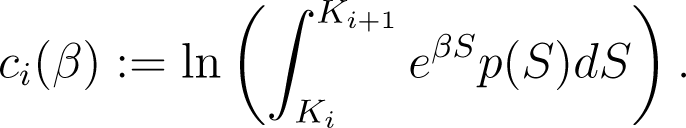
We define the cumulant generating functions c₀, …, c_n, from ℝ to ℝ ∪ {∞}, by

(8)

Notice that c_i(β) < ∞, for i < n and β ∈ ℝ, since p ∈ L¹(K_i, K_i+1) and the exponential function belongs to L^∞(K_i, K_i+1). For i = n, the integral is over [K_n, ∞) and we can have c_n(β) = ∞. However, c_n(0) < ∞ and if $e^{\widehat{\beta }S}p(S)$ belongs to L¹(K_n, ∞), then so does e^βSp(S) for $\beta <\widehat{\beta }$. Therefore, the interior of c_i’s effective domain is an interval of the form (−∞, β ) for some β  ≥ 0 and, for i < n, β  = ∞. Moreover, $c_i^{″}>0$.

Proposition 1

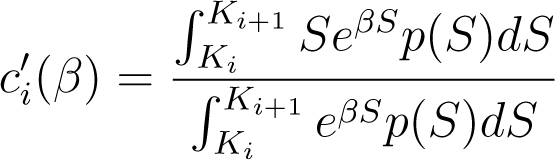
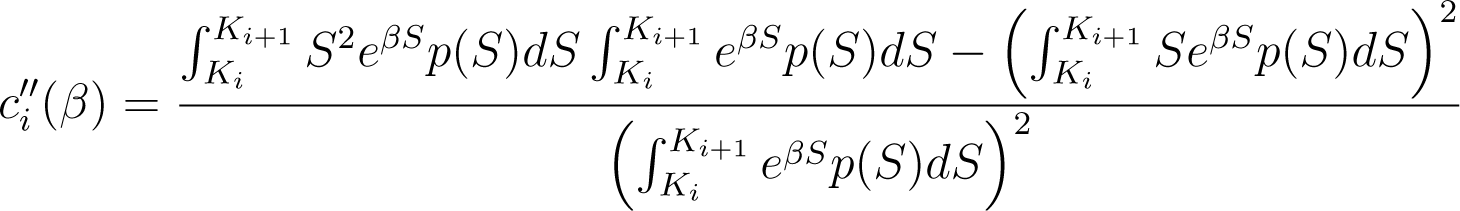
For i < n, c_i is twice differentiable and strictly convex in (−∞, β ). Moreover, its first and second derivatives are given by

(9)

and

(10)

for all β ∈ (−∞, β ).

Proof

Through standard arguments using the Mean Value Theorem and Lebesgue’s Dominated Convergence Theorem, one can show that for any $m\in \mathbb{Z}\cap [0,\infty )$, the function

$$w(\beta ):={\displaystyle {\int }_{K_i}^{K_{i+1}}{S}^m{e}^{\beta S}p(S)dS}$$

is differentiable in (−∞, β ) and its derivative can be obtained by differentiating under the integral sign. The differentiability of c_i and $c_i^{\prime }$ together with Equations (9) and (10) follows immediately.

Now we shall prove that $c_i^{″}>0$. We start by noticing that

$${\displaystyle {\int }_{K_i}^{K_i+1}{\displaystyle {\int }_{K_i}^{K_i+1}{(S-R)}^2{e}^{\beta (S+R)}p(S)p(R)dSdR>0.}}$$

(11)

Hence,

The left hand side of this last inequality can be rewritten as

or, simply as

whereas its right hand side is equal to

Therefore, the inequality (11) is equivalent to $c_i^{″}>0$.□

Introducing

(12)

and using Equation (8) we can rewrite Equations (6) and (7) in the simpler forms

$$c_i^{\prime }({\beta }_i)={\overline{K}}_i,$$

(13)

$${\alpha }_i=p_i{e}^{-c_i({\beta }_i)}.$$

(14)

Equation (13) is easily solved for β_i with the Newton–Raphson method using Equations (9) and (10). Once the density q has been obtained in this manner, i.e., α_i, β_i have been calculated for i = 0, …, n, we can calculate European option prices using numerical integration.

The next results give the existence and uniqueness of such β_i and, consequently, α_i.

Lemma 1

Let$m\in \mathbb{Z}\cap [0,\infty )$ Then, for any K ∈ (K_i, K_i+1) we have

Proof

We shall consider only the limit when β → ∞ since the other is treated analogously. Choose L and M such that K < L < M < K_i+1. Then, we have

Applying the First Mean Value Theorem for Integration yields S₁ ∈ [K_i, K] and S₂ ∈ [L, M] such that

Therefore

where C > 0 does not depend on β. Since S₁ − S₂ ≤ K − L < 0, the result follows.□

Proposition 2

We have${\lim }_{\beta \to \infty }{c}_i^{\prime }(\beta )=K_{i+1}$ and${\lim }_{\beta \to -\infty }{c}_i^{\prime }(\beta )=K_i$.

Proof

Here again, we only consider the first limit since the other is treated analogously. For all K ∈ (K_i, K_i+1) we have

Using the previous Lemma, we obtain that the term inside square brackets goes to 1 as β → ∞. Now we shall consider the last term above and show that, by choosing a suitable K, it is as close to K_i+1 as we want.

Firstly, we assume i < n. Then K_i+1 < ∞ and, given a small ε > 0, we choose K = K_i+1 − ε. The First Mean Value Theorem for Integration gives S₁ ∈ [K_i+1 − ε, K_i+1] such that

Now, for i = n, we have K_i+1 = ∞ and

Hence, the term above goes to K_i+1 = ∞ as K goes to ∞.□

Corollary 1

For all i = 0, …, n, under the non-arbitrage condition$K_i<{\tilde{K}}_i<K_{n+1}$, where${\tilde{K}}_i$ is defined in Equation (12), there exists a unique solution β_i ∈ ℝ of Equation (13).

Proof

Proposition 1 gives that $c_i^{\prime }$ is continuous and the last Proposition states that ${\lim }_{\beta \to -\infty }{c}_i^{\prime }(\beta )=K_i$ and ${\lim }_{\beta \to \infty }{c}_i^{\prime }(\beta )=K_{i+1}$. Hence the existence follows from the Intermediate Value Theorem. Additionally, Proposition 1 also gives that $c_i^{\prime }$ is strictly increasing and the uniqueness follows.□

Theorem 1

For all i = 0,…, n, let α_i and β_i be defined by Equations (13) and (14). Then q : [0, ∞) → ℝ given by

$$\begin{array}{cc}q(S)={\alpha }_i{e}^{{\beta }_{i}S}p(S)& \forall S\in [K_i,K_{i+1})\end{array}$$

minimises H(q||p).

Proof

This is shown just as Theorem 2.6 in [25] by using Theorem 2.5 by Csiszár also stated there. □

3.1. The Special Case of Non-Relative Entropy

The non-relative entropy can be seen as special case of the relative entropy for which no prior p is given or, roughly speaking, the prior is given by Lebesgue-measure p ≡ 1. Then Equation (8) reduces to the following analytic expression:

and the first and second derivatives given in Equations (9) and (10) reduce to

and

Using these expressions instead of Equations (8)–(10) allows for numerical integration to be avoided in an implementation in this case.

4. Minimiser Matching Call Option Prices

Buchen and Kelly describe in [6] a multi-dimensional Newton-Raphson algorithm to find the maximum entropy distribution (MED) if only call prices are given as constraints. The entropy H of a probability density q over [0, ∞) is given by

$$H(q)=-{\displaystyle {\int }_0^{\infty }q(S)\ln q(S)dS}.$$

In [13], we show how the results of [25] together with the Legendre transform can be applied to obtain a fast and more robust Newton–Raphson algorithm to calculate the Buchen–Kelly MED. The main reason that the algorithm is more stable is that the Hessian matrix has a very simple tridiagonal form. In Section II.A of their paper, Buchen and Kelly also consider the case of “minimum cross entropy” (which we call relative entropy here) for a given prior density.

We now show how essentially the same algorithm as that in [13] can be applied to the relative entropy case. The next proposition consolidates and generalises the results of Section 4 of [13], describing the entropy H, the gradient vector and the Hessian matrix to the case in which a prior density p is given.

Arbitrage free digital prices must lie between left and right call spread prices, i.e.,

(15)

where the rightmost quantity for i = n must be read as zero.

We introduce the set Ω ⊂ ℝⁿ of all $\tilde{D}=({\tilde{D}}_1,\dots ,{\tilde{D}}_n)\in {ℝ}^n$ verifying Equation (15). Note that Ω is an open n-dimensional rectangle. Define $q_{\tilde{D}}$ as the density obtained as in Theorem 1 for given (undiscounted) digital prices $\tilde{D}$.

Proposition 3

For all$\tilde{D}\in \Omega$ the relative entropy of$q_{\tilde{D}}$ with respect to p can be expressed as

$$H(q_{\tilde{D}}\parallel p)={\displaystyle \sum _{i=0}^n{p}_i\ln p_i+}{\displaystyle \sum _{i=0}^n{p}_i}{c}_i^{*}({\overline{K}}_i),$$

where$c_i^{*}$ is the Legendre transform of c_i, $p_i:={\tilde{D}}_i-{\tilde{D}}_{i+1}$ and${\overline{K}}_i$ is given by Equation (12).

As a function of digital prices, H : Ω → ℝ is strictly convex, twice differentiable and, for all$\tilde{D}\in \Omega$, we have

$$\begin{array}{cc}\frac{\partial H}{\partial {\tilde{D}}_i}(\tilde{D})=\ln g_{\tilde{D}}(K_i+)-\ln g_{\tilde{D}}(K_i-),& \forall i=1,\dots ,n\end{array},$$

where$g_{\tilde{D}}:=q_{\tilde{D}}/p$ and

with α_i and β_i given by Equations (13) and (14), for all i = 0,…, n.

In addition, the Hessian matrix at any$\tilde{D}\in \Omega$ is symmetric and tridiagonal with entries given by

Proof

Let $g_{\tilde{D}}:=q_{\tilde{D}}/p$ be the piecewise-exponential Radon–Nikodým derivative given in Theorem 1. We have

since $g_{\tilde{D}}(S)={\alpha }_i{e}^{{\beta }_{i}S}$ on [Ki, K_i+1). Then using Equations (13) and (14) the proof goes through as the proofs of Theorem 4.1, Theorem 4.2, Lemma 5.1 and Proposition 5.2 from [13] given there by using the generalised versions of c_i and $c_i^{*}$ introduced above and observing the absence of the minus sign in the definition of relative entropy.□

Notice that p_i and ${\overline{K}}_i$ are given purely in terms of option prices, for all i = 0,…, n, and so is $H(q_{\tilde{D}}\parallel p)$ Notice also that if the prior density p already matches the call prices, then α_i = 1 and β_i = 0 for all i = 0,…,n. From the relationship $c_i^{*}({\overline{K}}_i)={\beta }_i{\overline{K}}_i-c_i({\beta }_i)$, it follows that, in this case, $c_i^{*}({\overline{K}}_i)=-c_i({\beta }_i)$. Since $\ln p_i=\ln {\alpha }_i+c_i({\beta }_i)=-c_i^{*}({\overline{K}}_i)$, the proposition above gives that $H(q_{\tilde{D}}\parallel p)=0$, as expected.

The expression for the derivative of H gives that if $\tilde{D}$ minimises H (i.e., $\tilde{D}$ is a root of the gradient of H), then $g_{\tilde{D}}$ is continuous. Furthermore, the MRED $q_{\tilde{D}}=g_{\tilde{D}}p$ has the same points of discontinuity as p.

Using these last results, essentially the same Newton–Raphson algorithm as in [13] can be applied to find the relative entropy minimiser q. The only differences are that the functions $c_0^{″},\dots ,c_n^{″}$ must be replaced by their relative entropy versions Equation (10) in the Hessian matrix of Proposition 3, and that in each iteration step, for a given set of digital prices, the algorithm of Section 3 must be used to calculate the MRED, instead of its non-relative version.

5. Probability Densities for Characteristic Function Models

In this section, we look at four models that are popular in equity derivatives pricing. Our aim is to use the densities they give for the stock price at a fixed maturity as prior densities. In two of the models we have chosen, the Black–Scholes model and the Variance Gamma model, the density is analytically available. In the other two, the Heston and the Schöbel–Zhu stochastic volatility models, it is not. We therefore give a brief overview of these models and show how to calculate their densities in each case.

Let $\tilde{p}$ be the density of x(T) := ln S(T). To simplify notation, we will usually write x and S, respectively, when it is clear from the context that we have fixed the maturity T. Then the density p of S itself is given by

$$p(S)=\frac{1}{S}\tilde{p}(\ln S),$$

since ${\displaystyle {\int }_{-\infty }^{\ln a}\tilde{p}(x)dx={\displaystyle {\int }_0^a\tilde{p}(\ln S)\frac{1}{S}dS=}{\displaystyle {\int }_0^{a}p(S)dS}}$ by change-of-variables formula.

If the characteristic function ϕ of $\tilde{p}$, given by

$$\varphi (u):=\mathbb{E}\left[e^{iux}\right]={\displaystyle {\int }_{-\infty }^{\infty }{e}^{iux}\tilde{p}(x)dx,}$$

(16)

is known, as in the Heston [32] or Schöbel–Zhu [33] stochastic volatility models, then $\tilde{p}$ can be obtained via Fourier inversion:

$$\tilde{p}(x)=\frac{1}{2\pi }{\displaystyle {\int }_{-\infty }^{\infty }{e}^{-}{}^{iux}\varphi (u)du.}$$

Since $\tilde{p}$ is a real-valued function, it follows from Equation (16) that $\varphi (-u)=\overline{\varphi (u)}$, and we have

(17)

where $\Re [z]=(z+\overline{z})/2$ denotes the real part of a complex number z. It can immediately be seen that an anti-derivative of $\tilde{p}$ is given by

$${\tilde{p}}_0(x)=-\frac{1}{2\pi }{\displaystyle {\int }_{-\infty }^{\infty }\frac{e^{-}{}^{iux}}{iu}\varphi (u)du.}$$

Furthermore, it can be shown in a similar way as the Fourier Inversion Theorem itself, that ${\lim }_{x\to -\infty }{\tilde{P}}_0(x)=-\frac{1}{2}$ and ${\lim }_{x\to \infty }{\tilde{P}}_0(x)=\frac{1}{2}$, and therefore the function

gives an expression for the distribution function.

For pricing, we use the general formulation of Bakshi and Madan [34]. This can be used for a large class of characteristic function models that contains the Heston, Schöbel–Zhu and Variance Gamma models (see Section 2 in [34], in particular Case 2 on p. 218). We have S > K if, and only if, x > ln K.

Let

(18)

(19)

represent the probabilities of S finishing in-the-money at time T in case the stock S itself or a risk-free bond is used as numéraire, respectively. From Equation (16) we can see that $\varphi (-i)=\mathbb{E}[e^x]=\mathbb{E}[S]$, so that the quotient

$$\frac{\varphi (u-i)}{\varphi (-i)}={\displaystyle {\int }_{\infty }^{\infty }{e}^{iux}\frac{S}{\mathbb{E}[S]}}p(x)dx$$

contains the appropriate change of measure.

The price C of a European call option on a stock paying a dividend yield d is then obtained through

$$C=e^{-dT}S{\prod }_1-e^{-rT}K{\prod }_2,$$

(20)

and the price D of a European digital call option prices through

$$D=e^{-rT}{\prod }_2,$$

(21)

where r is the risk-free, continuously-compounded interest rate.

The integrals in Equations (17)–(19) must of course be truncated at some point a, which depends on the decay of the characteristic function of the model considered.

5.1. The Black-Scholes Model

Let the parameters r, d and T be given as above, and let σ > 0 be the volatility of the stock price. In the Black–Scholes model, the logarithm x(t) := ln S(t) follows the SDE

$$dx(t)=(r-d-\frac{1}{2}{\sigma }^2)dt+\sigma dW(t),x(0)=\ln S(0).$$

Define $\mu :=x(0)+(r-d-\frac{1}{2}{\sigma }^2)T$.

The density of x := x(T) is normal and given by

$$\tilde{p}(x)=\frac{1}{\sqrt{2\pi {\sigma }^{2}T}}{e}^{-\frac{{(x-\mu )}^2}{2{\sigma }^{2}T}}.$$

(22)

The characteristic function of $\tilde{p}$ has a very simple form and is given by

$$\varphi (u)=e^{iu\mu -\frac{1}{2}{u}^2{\sigma }^{2}T}.$$

(23)

Of course it is faster to use Equation (22) directly instead of Equations (23) and (17), but comparing these two methods lets one measure the additional computational burden.

5.2. The Heston Model

One of the most popular models for derivative pricing in equity and foreign exchange (FX) markets is the stochastic volatility model introduced by Heston [32]. Let x(t) := ln S(t). The model is given, in the risk-neutral measure, by the following two SDE’s:

$$dx(t)=(r-d\frac{1}{2}\upsilon (t))dt+\sqrt{\upsilon (t)}d{W}_1(t),x(0)=\ln S(0),$$

(24)

$$d\upsilon (t)=(\kappa \theta -(\kappa +\mathrm{\lambda })\upsilon (t))dt+\sigma \sqrt{\upsilon (t)}d{W}_2(t),\upsilon (0)={\upsilon }_0,$$

(25)

where 〈dW₁(t), dW₂(t)〉 = ρdt. The variance rate v follows a Cox–Ingersoll–Ross square-root process [35].

The parameter λ represents the market price of volatility risk. Since we are only interested in pricing, we always set λ = 0 in what follows (see Chapter 2 in Gatheral [28]).

Heston calculates the characteristic function solution, but as pointed out in [33], there is a (now well-known) issue when taking the complex logarithm. To be clear, we therefore give the formulation of the characteristic function that we use.

Define

(26)

Introducing

the characteristic function of x(T) is then given as

$$\varphi (u)=e^{C+D\upsilon (0)+iux(0)}.$$

(27)

Since implementations of the complex square-root usually return the root with non-negative real part (d₁), the key is simply to take the other root (d₂), as is done in Equation (26). As shown in [36,37], this takes care of the whole issue.

5.3. The Schöbel–Zhu Model

The Schöbel–Zhu model [33] is an extension of the Stein and Stein stochastic volatility model [38] with correlation ρ ≠ 0 allowed (see also [39,40]). It is described, in the risk-neutral measure, by the following two SDE’s:

$$dx(t)=(r-d-\frac{1}{2}{\upsilon }^2(t))dt+\upsilon (t)d{W}_1(t),x(0)=\ln S(0),$$

(28)

$$d\upsilon (t)=\kappa (\theta -\upsilon (t))dt+\sigma d{W}_2(t),\upsilon (0)={\upsilon }_0,$$

(29)

where 〈dW₁(t), dW₂(t)〉 = ρdt. The volatility υ follows a mean-reverting Ornstein–Uhlenbeck process.

The characteristic function for this model is given by Schöbel and Zhu in [33]. As Lord and Kahl point out (Section 4.2 in [37]), similar attention has to be paid when taking the complex logarithm in this model’s characteristic function as in Heston’s. By directly relating the two characteristic functions (Equation 4.14 on p.682 of [37]), they show how the Schöbel–Zhu model can also be implemented safely. In the case study in Section 6.2 presented in the following section with SPX option data and a maturity of less than half a year, however, we observed no problems with the characteristic function originally proposed by Schöbel and Zhu.

5.4. The Variance Gamma Model

The Variance Gamma (VG) process was introduced in [41,42]. The density for x = ln S(T) is given explicitly in Theorem 1 in [41]. Define x₀ = ln S(0),

$$\omega :=\frac{1}{\nu }\ln (1-\theta \nu -\frac{1}{2}{\sigma }^2\nu )and\tilde{x}=x-x_0-(r-d+\omega )T.$$

Then the density $\tilde{p}$ is given by

(30)

where Γ is the Gamma-function and K is the modified Bessel function of the second kind.

If the parameter ν is set to zero, the characteristic function of p reduces to the Black–Scholes one given in Equation (23). Otherwise, it is given by

$$\varphi (u)=e^{iu(x_0+(r-d+\omega )T)}{\left(1-i\theta \nu u+\frac{1}{2}{\sigma }^2{u}^2\nu \right)}^{\frac{T}{\nu }}.$$

(31)

Lord and Kahl show (Section 4.1 in [37]) that this formulation of the characteristic function is safe.

Again, as with the Black–Scholes model, since both the density and the characteristic function are available, it is possible to compare the two different methods Equation (30) vs. Equations (31) and (17).

6. Two Numerical Examples

6.1. A Fictitious Market and Black–Scholes and Heston Prior Densities

In our first example, we take a hypothetical market with r = d = 0,T = 1, S = F = 100, in which call option prices are given by the Black–Scholes formula with volatility σ = 0.25. As prior densities, we take

• p_bs, a Black–Scholes log-normal density, but this time with volatility σ_p = 0.20,

• p_h, a Heston density, with parameters κ = 1, θ = 0.04, ρ = −0.3, σ = 0.25, υ₀ = 0.04, which leads to implied volatilities of 0.2418,0.2125,0.1923,0.1855,0.1884 at strikes 60, 80,100,120,140, respectively.

We calculate the Buchen–Kelly MED (Lebesgue prior), using the algorithm presented in [13], and the two Buchen–Kelly MREDs with priors p_bs and p_H, using the generalised algorithm presented in Section 4, and compare the resulting call and digital option prices to see the influence of the priors. Note that to obtain the density of the Heston model, we evaluate the integral in Equation (17) up to a = 250.

The different call and digital option prices are reported in

Table 1. Comparison of call and digital prices.

Strike	Call Prices			Digital Prices
	MED BK	MRED BS	MRED Heston	MED BK	MRED BS	MRED Heston
20	80.0538	80.0000	80.0000	0.9936	1.0000	1.0000
40	60.3244	60.0000	60.0094	0.9766	1.0000	0.9979
60	41.1698	40.0637	40.3043	0.9316	0.9841	0.9595
80	23.5389	21.9716	22.5717	0.8124	0.7758	0.7828
100	9.9476	9.9476	9.9476	0.4962	0.4420	0.4763
120	3.6684	3.6071	3.3294	0.1830	0.2039	0.1977
140	1.3528	1.0596	1.0051	0.0675	0.0693	0.0593
160	0.4989	0.2688	0.3239	0.0249	0.0192	0.0175
180	0.1840	0.0621	0.1171	0.0092	0.0047	0.0056
20	80.0000	80.0000	80.0000	1.0000	1.0000	1.0000
40	60.0015	60.0003	60.0012	0.9997	0.9998	0.9996
60	40.1454	40.1454	40.1454	0.9669	0.9753	0.9715
80	22.5812	22.0890	22.3433	0.7743	0.7818	0.7770
100	9.9476	9.9476	9.9476	0.4646	0.4424	0.4633
120	3.7041	3.7051	3.5189	0.1945	0.1976	0.1926
140	1.2139	1.2139	1.2139	0.0705	0.0707	0.0617
160	0.3800	0.3569	0.4669	0.0221	0.0227	0.0207
180	0.1190	0.0961	0.2067	0.0069	0.0065	0.0077
20	80.0001	80.0000	80.0000	1.0000	1.0000	1.0000
40	60.0033	60.0002	60.0014	0.9994	0.9999	0.9996
60	40.1454	40.1454	40.1454	0.9726	0.9727	0.9726
80	22.2656	22.2656	22.2656	0.7794	0.7781	0.7804
100	9.9476	9.9476	9.9476	0.4510	0.4499	0.4510
120	3.7059	3.7059	3.7059	0.1971	0.1961	0.1958
140	1.2139	1.2139	1.2139	0.0700	0.0711	0.0689
160	0.3834	0.3545	0.4105	0.0221	0.0227	0.0211
180	0.1211	0.0948	0.1564	0.0070	0.0064	0.0071

. The densities were calculated using call prices at strikes

• k₀ = 0, K₁ = 100

• k₀ = 0, K₁ = 60, K₂ = 100, K₃ = 140

• k₀ = 0, K₁ = 60, K₂ = 80, K₃ = 100, K₄ = 120, K₅ = 140

as respective constraints. These strikes are the ones in boldface in Table 1.

We see that in the first case, where we had only the forward and an at-the-money call option as constraints, there are significant differences in both call and digital prices. The presence of the log-normal prior density makes MRED BS call prices cheaper compared with the original BS prices. Of course, under the prior density itself, call prices were cheaper because of the lower volatility, and this effect seems to persist. We also see that the fatter (exponential) tails of the MED translate into higher prices of deeply in- or out-of-the-money call options when compared with the other two densities.

However, as we add call prices at more strikes as constraints, the differences become smaller. In the third part of Table 1, the prices of both call and digital options are clearly converging.

6.2. SPX Option Prices and Heston, Schöbel–Zhu and VG Prior Densities

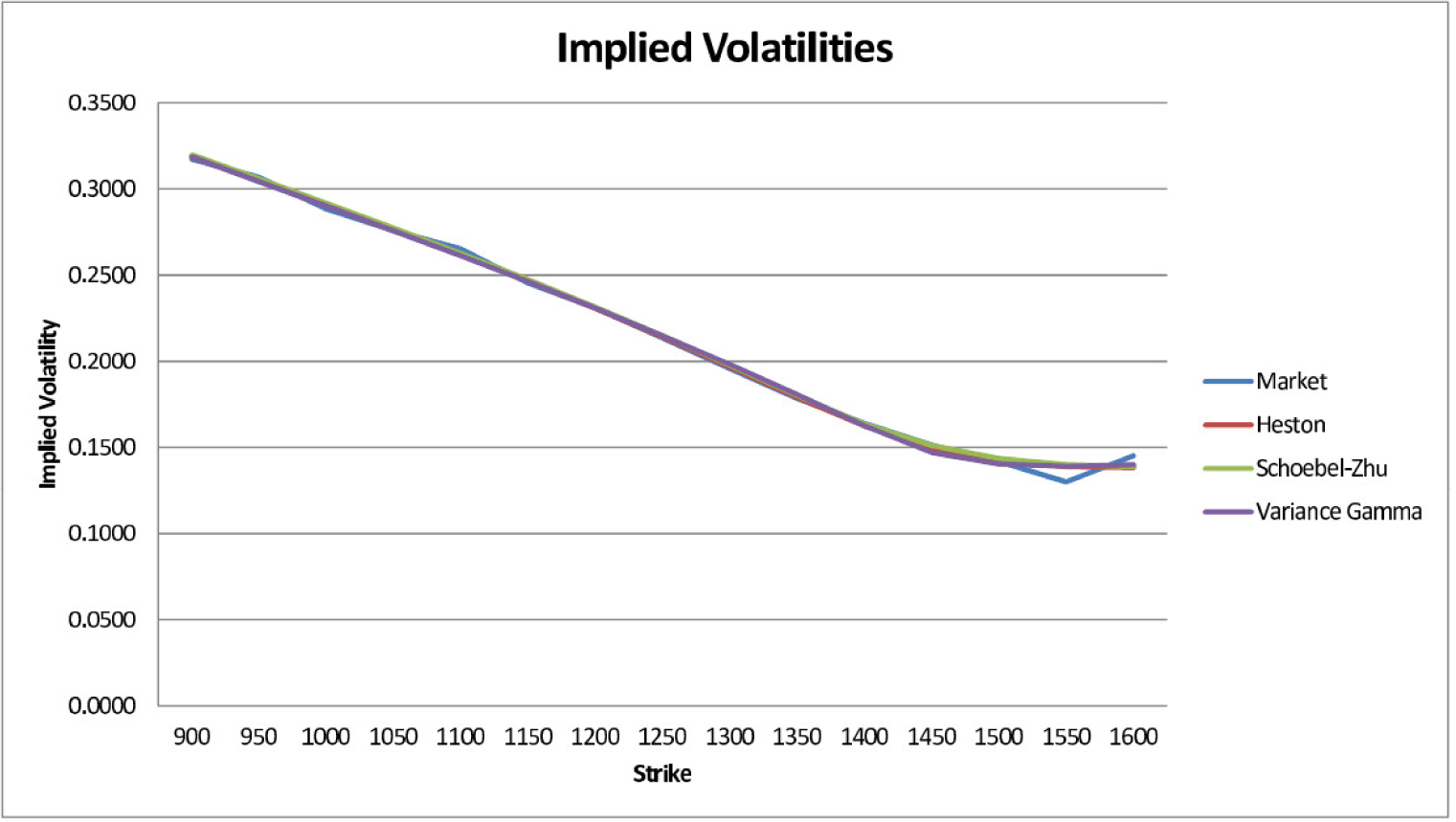
In our second example, we look at call (ticker symbol SPX) and digital (BSZ) options on the Standard and Poor’s 500 stock index [43]. The market data is from 18 July 2011. We consider those options that expire on 17 December 2011 and calibrate a Heston, Schöbel–Zhu and VG model, respectively, to call prices for 15 strikes 900, 950, …1550, 1600 at constant intervals of 50 using a Levenberg–Marquardt least-squares method ([39,44]). To evaluate the densities via Equation (17), we use α_Heston = α_SZ = 250 and α_VG = 1000. The model parameters we obtained are given in

Table 2. Model parameters.

Parameter	Heston	SZ	VG
κ	0.8568	1.6316	n/a
θ	0.0800	0.1731	−0.2808
ρ	−0.8016	−0.8031	n/a
σ	0.5473	0.3249	0.1535
υ0	0.0421	0.1887	n/a
v	n/a	n/a	0.3638

.

Figure 1 shows the market implied volatility skew and the volatility skews generated by the three models. Apart from the last two strikes at 1550 and 1600, the fit looks quite good in all three cases:

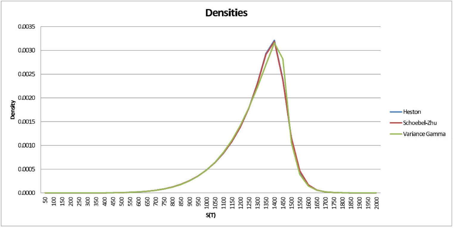
Using formulas for the densities directly, if available, or otherwise the numerical inversion formula given in Equation (17), we plot the densities for S(T) given by these models in Figure 2:

The Heston and Schöbel–Zhu densities are almost indistinguishable from one another, whereas the VG density has a somewhat different shape with a slightly thinner right tail.

Table 3. Squared errors and relative entropy H(h||p).

Model:	Heston	SZ	VG
${\displaystyle \sum {({\sigma }_i-{\widehat{\sigma }}_i)}^2:}$	1.59 × 10−4	1.86 × 10−4	1.74 × 10−4
Relative Entropy:	0.1311	0.1315	0.1374

shows the sum of squared errors ${{\displaystyle {\sum }_{i=1}^{15}({\sigma }_i^{SPX}-{\widehat{\sigma }}_i^{model})}}^2$ between the market (SPX) implied volatilities and the model implied volatilities. The relative entropy H(q||p) can be seen as an alternative measure of fit, since by Equation (2) it measures how much the prior density p needs to be deformed to obtain a density q that perfectly matches the given market data. Interestingly, the Heston model fits best under either criterion, but the order of the Schöbel–Zhu and VG models is reversed in the two cases.

Finally, digital prices are reported in

Table 4. Digital prices.

Strike	Market (Mid)	Call Spreads	MED BK	Heston	MRED Heston	SZ	MRED SZ	VG	MRED VG
900	0.9500	0.9560	0.9609	0.9682	0.9612	0.9678	0.9612	0.9687	0.9607
950	0.9500	0.9540	0.9544	0.9532	0.9544	0.9527	0.9544	0.9537	0.9544
1000	0.9400	0.9335	0.9432	0.9325	0.9433	0.9319	0.9433	0.9331	0.9432
1050	0.9100	0.8935	0.8830	0.9048	0.8830	0.9041	0.8830	0.9052	0.8830
1100	0.8800	0.8685	0.8695	0.8683	0.8695	0.8675	0.8695	0.8679	0.8695
1150	0.8300	0.8250	0.8409	0.8207	0.8409	0.8198	0.8409	0.8191	0.8409
1200	0.7700	0.7555	0.7520	0.7595	0.7520	0.7585	0.7520	0.7560	0.7520
1250	0.6850	0.6810	0.6893	0.6809	0.6893	0.6797	0.6893	0.6759	0.6893
1300	0.5850	0.5745	0.5797	0.5792	0.5797	0.5783	0.5797	0.5756	0.5797
1350	0.4550	0.4365	0.4386	0.4482	0.4388	0.4481	0.4388	0.4527	0.4383
1400	0.3100	0.2885	0.2855	0.2913	0.2858	0.2924	0.2858	0.3060	0.2867
1450	0.1700	0.1605	0.1505	0.1464	0.1502	0.1489	0.1502	0.1443	0.1485
1500	0.0700	0.0743	0.0714	0.0590	0.0714	0.0616	0.0714	0.0537	0.0718
1550	0.0350	0.0235	0.0121	0.0216	0.0118	0.0230	0.0117	0.0201	0.0118
1600	0.0300	0.0025	0.0009	0.0077	0.0010	0.0082	0.0011	0.0077	0.0010

. There are noticeable differences between market prices (although these must be taken with a pretty big pinch of salt due to the poor liquidity and large bid-ask spreads), the Buchen–Kelly prices and the prices given by the three models. However, regarding the three relative entropy distributions obtained using the different model priors, it seems that the effect of the prior density on digital prices is negligible: all three MREDs basically agree with the Buchen–Kelly MED.

7. Variance Swaps

In this section we recall the definition of a variance swap and the pricing formula based on replication through a log contract. (For more details see [26,27,45] and references therein.)

A variance swap is a forward contract on the annualised realised variance of the underlying asset over a period of time. More precisely, given observation dates $t_0<\cdots <t_m$, the realised variance is defined by

$${\sigma }_{\text{real}}^2:=\frac{252}{m}{{\displaystyle \sum _{i-1}^m\left[\ln \left(\frac{S(t_i)}{S(t_{i-1})}\right)\right]}}^2,$$

where S(t) denotes the spot price of the underlying asset at time t. The number 252 above is the annualisation factor and reflects the typical number of business days in a year. The payoff of a variance swap is given by

$$N\cdot ({\sigma }_{\text{real}}^{\text{2}}-K_{\text{var}}),$$

where K_var is the strike price for variance and N is the notional amount of the swap.

Assume that {S(t)}_t≥0 follows a stochastic differential equation

$$\frac{dS(t)}{S(t)}=\mu (t)dt+\sigma (t)dB(t),$$

(32)

where {B(t)}_t≥0 is a standard Brownian motion and the drift {µ(t)}_t≥0 and the volatility {σ(t)}_t≥0 are stochastic processes adapted to the (possibly enlarged) natural filtration ${ℱ}^B={({ℱ}_t^B)}_{t\ge 0}of{\{B(t)\}}_{t\ge 0}$. (The hypothesis on {σ(t)}_t≥0 can be relaxed to allow a larger class of processes by enlarging $ℱ$^B to a filtration $\mathscr{H}$ ⊃ $ℱ$^B such that B is an $\mathscr{H}$-martingale and {σ(t)}_t≥0 is $\mathscr{H}$-adapted. This formulation then includes stochastic volatility models that are solutions of multi-dimensional SDEs, and $\mathscr{H}$ can be taken as the natural filtration of the multi-dimensional Brownian motion.)

Typically, K_var is such that the theoretical price of the variance swap is null at inception and, in this case, it is said to be the fair variance swap rate and denoted by ${\sigma }_{\text{fair}}^2$. The theoretical realised variance over the period [0, T], and so ${\sigma }_{\text{fair}}^2$, is given by

$${\sigma }_{\text{fair}}^2:=\frac{1}{T}\mathbb{E}\left[{\displaystyle {\int }_0^T\sigma {(t)}^{2}dt}\right].$$

We shall now derive a formula for ${\sigma }_{\text{fair}}^2$ based on the price of a log contract, that is, a derivative whose payoff at maturity T is ln S(T). Let x(t) := ln S(t) and apply Itô’s formula to obtain

$$dx(t)=\left(\mu (t)-\frac{1}{2}{\sigma }^2(t)\right)dt+\sigma (t)dB(t).$$

(33)

Subtracting Equation (33) from Equation (32) gives

$$\frac{dS(t)}{S(t)}-dx(t)=\frac{1}{2}{\sigma }^2(t)dt.$$

(34)

Integrating from 0 to T and multiplying by 2/T gives

Finally, taking expectations yields

$${\sigma }_{\text{fair}}^2=\frac{2}{T}\mathbb{E}\left[{\displaystyle {\int }_0^T\mu (t)dt}\right]+\frac{2}{T}\ln S(0)-\frac{2}{T}\mathbb{E}[\ln S(T)],$$

(35)

since $\mathbb{E}\left[{\displaystyle {\int }_0^T\sigma (t)dB(t)}\right]=0$. Notice that $\mathbb{E}\left[\ln S(T)\right]$ is the price of a log contract.

7.1. Maximum Entropy and Variance Swaps

In this section, we shall derive a relationship between the fair swap rate of a variance swap and the entropy of the underlying asset density. This relationship follows from another one relating the entropies of the density q of a random variable S and the density of x := ln S, which is the subject of the next proposition.

Proposition 4

The (non-relative) entropy H(q) of a density q of a random variable S on (0, ∞) and the entropy$\tilde{H}(\tilde{q})$ of the density$\tilde{q}$ of x := ln(S) on (−∞, ∞) are related by

$$\tilde{H}(\tilde{q})-H(q)=\mathbb{E}\left[x\right].$$

(36)

Proof

Recall that the densities q and $\tilde{q}$ are related by

$$q(S)=\frac{1}{S}\tilde{q}(\ln S)=\tilde{q}(x)e^{-x}.$$

Hence, the change of measure dS = e^xdx gives

Corollary 2

Consider an asset whose price S(t) at time t follows Equation (32). Let q be the density of S(T), for some T > 0, and$\tilde{q}$ be the density of x(T) := ln S(T). Then the fair variance swap rate of a variance swap maturing at time T is given by

$${\sigma }_{\text{fair}}^2=\frac{2}{T}\mathbb{E}\left[{\displaystyle {\int }_0^T\mu (t)dt}\right]+\frac{2}{T}\ln S(0)-\frac{2}{T}\left(\tilde{H}(\tilde{q})-H(q)\right).$$

(37)

Proof

This follows immediately from the last proposition and Equation (35).

When the density q of S(T) is known, the price of a log contract $\mathbb{E}\left[\ln S(T)\right]$ can be computed through numerical integration. Moreover, when q is the MED, that is, in the non-relative entropy case, we show how this price can be computed analytically. By definition, the expectation is given by

$$\mathbb{E}[\ln S(T)]={\displaystyle {\int }_0^{\infty }\ln (S)q(S)dS}={\displaystyle \sum _{i=0}^n{\alpha }_i{\displaystyle {\int }_{K_i}^{K_{i+1}}\ln (S)e^{{\beta }_{i}S}dS.}}$$

For i ∉ {0, n} and βi ≠ 0 we have

$${\alpha }_i{\displaystyle {\int }_{K_i}^{K_{i+1}}\ln (S)e^{{\beta }_{i}S}dS}=\frac{{\alpha }_i}{{\beta }_i}{[e^{{\beta }_{i}S}\ln S-Ei({\beta }_{i}S)]}_{K_i}^{K_i+1},$$

(38)

where $Ei(s):=-{\displaystyle {\int }_{-s}^{\infty }\frac{e^{-t}}{t}}dt$ is the exponential integral function. Note that if β_i = 0, then of course

$${\displaystyle {\int }_{K_i}^{K_{i+1}}\ln (S)e^{{\beta }_{i}S}dS}={\displaystyle {\int }_{K_i}^{K_{i+1}}\ln (S)dS}={[S\ln S-S]}_{K_i}^{K_i+1}.$$

The exponential integral function has a pole at 0, and therefore we cannot evaluate Equation (38) directly at K₀ = 0. From the series representation

$$Ei(s)=\mathrm{\gamma }+\ln \left|s\right|+{\displaystyle \sum _{k=1}^{\infty }\frac{s^k}{kk!},s\ne 0,}$$

it follows that we have in the limit

$$\underset{S\to 0}{\lim }{e}^{{\beta }_{0}S}\ln S-Ei({\beta }_{0}S)=-\mathrm{\gamma }-\ln \left|{\beta }_0\right|,$$

where γ = 0.5772156649… is the Euler–Mascheroni constant. At the other extreme, at K_n+1 = ∞, we have in the limit

$$\underset{S\to 0}{\lim }{e}^{{\beta }_{n}S}\ln S-Ei({\beta }_{n}S)=0,$$

since β_n < 0. Putting this together gives a closed formula for Equation (36).

7.2. Numerical Examples

In the first example, the market is given as in Section 6.1 by a Black-Scholes model with volatility σ = 0.25, with the same sets of 1, 3 and 5 strikes.

Table 5. Fair variance swap rate and entropy.

MED	1 Strike	3 Strikes	5 Strikes
σfair	0.3130	0.2545	0.2506
${\sigma }_{\text{fair}}^2$	0.0980	0.0647	0.0628
Entropy	4.6801	4.6165	4.6077

shows three quantities obtained from (non-relative) Buchen-Kelly MEDs fitted to the forward and call prices at these strikes: the fair variance swap rate ${\sigma }_{\text{fair}}^2$, its square-root for comparison with implied volatilities, and the entropy. The average volatility σ_fair and the entropy can be seen as two different measures of the dispersion of S(T). As the number of strikes increases, σ_fair and the entropy both decrease, with σ_fair converging towards the Black–Scholes volatility σ = 0.25.

In the second example, we use the same reference market as above, but now we include a prior Black–Scholes density and calculate the MREDs matching the forward and call prices at 1, 3 and 5 strikes. The prior density is characterised by its volatility σ_p.

Table 6. Black–Scholes prior and fair variance swap rate.

Prior	MRED 1 Strike		MRED 3 Strikes		MRED 5 Strikes
BS σp	σfair	${\sigma }_{\text{fair}}^2$	σfair	${\sigma }_{\text{fair}}^2$	σfair	${\sigma }_{\text{fair}}^2$
0.20	0.2427	0.0589	0.2476	0.0613	0.2497	0.0624
0.25	0.2500	0.0625	0.2500	0.0625	0.2500	0.0625
0.30	0.2559	0.0655	0.2514	0.0632	0.2502	0.0626
0.35	0.2608	0.0680	0.2523	0.0637	0.2503	0.0626
0.40	0.2650	0.0702	0.2529	0.0640	0.2503	0.0627
0.45	0.2688	0.0723	0.2533	0.0642	0.2504	0.0627
0.50	0.2723	0.0741	0.2536	0.0643	0.2504	0.0627

shows that increasing σ_p has the effect of increasing the fair variance swap rate of the MRED. However, we see that as we add more constraints, this effect is diminished. In the case of 5 strikes, it is barely noticeable. Note that in the case σ_p = 0.25 where the prior density already matches the given constraints, the MRED is equal to the prior, and we recover the volatility of the Black–Scholes process as the square-root of the fair variance swap rate.

In the third example, summarised in

Table 7. Heston prior and fair variance swap rate.

Prior	MRED 1 Strike		MRED 3 Strikes		MRED 5 Strikes
Heston σ	σfair	${\sigma }_{\text{fair}}^2$	σfair	${\sigma }_{\text{fair}}^2$	σfair	${\sigma }_{\text{fair}}^2$
0.10	0.2448	0.0599	0.2485	0.0618	0.2499	0.0624
0.20	0.2506	0.0628	0.2500	0.0625	0.2503	0.0627
0.30	0.2600	0.0676	0.2520	0.0635	0.2506	0.0628
0.40	0.2890	0.0835	0.2535	0.0643	0.2507	0.0629
0.50	0.3237	0.1048	0.2544	0.0647	0.2507	0.0629
0.60	0.3464	0.1200	0.2555	0.0653	0.2508	0.0629
0.70	0.3711	0.1377	0.2565	0.0658	0.2508	0.0629

, we proceed as in the second one, but now with a Heston density as the prior. The Heston parameters are the same as in Section 6.1, i.e., κ= 1, θ = 0.04, ρ = −0.3, υ₀ = 0.04, but now we vary the volatility σ of the variance and measure its impact on the fair variance swap rate of the MRED. In the case of 1 strike, we see clearly that this impact is very strong. However, we notice again that increasing the number of strikes quickly diminishes the strength of the impact.

8. Conclusions

In this article we generalise the algorithm presented in [13] to the relative entropy case. The algorithm allows for efficient computation of a risk-neutral probability density that exactly gives European call option prices quoted in the market, while staying as close as possible to a given prior density under the criterion of relative entropy.

It is not necessary to have an analytic expression for the prior density in question. In practice, several popular equity and FX models work through their characteristic functions and numerical Fourier inversion techniques. We pick two of these as examples, namely the Heston and the Schöbel–Zhu stochastic volatility models, and show how they nevertheless can be used to provide the prior density and incorporated into our algorithm. In other cases, analytic expressions for the density are available, such as for the Black–Scholes model and the Variance Gamma model (for example, in C++ this is easily implemented using the functions boost::math::tgamma and boost::math::cyl_bessel_k in Boost [46]), and we also incorporate these into our analysis.

As an application, we study the impact of the choice of prior density. In a first, purely hypothetical scenario, we assume that only the prices of a few options are quoted. We observe that using a prior density does indeed lead to significantly different option prices when compared with pricing with a pure log-normal density or a piece-wise exponential Buchen–Kelly density.

In a second scenario we use option price data for S&P500 index options for a fixed maturity traded on the CBOE. We calibrate three different models to these data and observe that, although the models generate noticeably different digital option prices, the prices obtained when using minimum relative entropy densities, with these models for the prior densities, agree almost perfectly. Furthermore, these prices are essentially the same as those given by the (non-relative) Buchen–Kelly density itself. In other words, in a sufficiently liquid market, the effect of the prior density seems to vanish almost completely.

We also study variance swaps and establish a formula that relates their fair swap rate to entropy. In the case of MEDs, we give an explicit formula for the fair swap rate. In the case of MREDs, we study the impact of the prior density on the fair swap rate and see that, again, while it has a substantial effect when constraints exist at only a very small number of strikes, this effect diminishes rapidly as more constraints are added.

References

- Boltzmann, L. Über die Beziehung zwischen dem zweiten Hauptsatze der mechanischen Wärmetheorie und der Wahrscheinlichkeitsrechnung respektive den Sätzen über das Wärmegleichgewicht. Wien. Akad. Sitz 1877, 76, 373–435. (in German). [Google Scholar]
- Shannon, C.E. On Information and Sufficiency. Bell Syst. Tech. J 1948, 27, 379. [Google Scholar]
- Kullback, S.; Leibler, R.A. On Information and Sufficiency. Ann. Math. Stat 1951, 22, 79–86. [Google Scholar]
- Csiszár, I. I-Divergence Geometry of Probability Distributions and Minimization Problems. Ann. Probab 1975, 3, 146–158. [Google Scholar]
- Rubinstein, R.Y.; Kroese, D.P. The Cross-Entropy Method: A Unified Approach to Combinatorial Optimization, Monte–Carlo Simulation and Machine Learning; Information Science and Statistics; Springer: New York, NY, USA, 2004. [Google Scholar]
- Buchen, P.W.; Kelly, M. The Maximum Entropy Distribution of an Asset Inferred from Option Prices. J. Financ. Quant. Anal 1996, 31, 143–159. [Google Scholar]
- Stutzer, M. A Simple Nonparametric Approach to Derivative Security Valuation. J. Financ 1996, 51, 1633–1652. [Google Scholar]
- Stutzer, M. A Bayesian Approach to Diagnosis of Asset Pricing Models. J. Econom 1995, 68, 367–397. [Google Scholar]
- Stutzer, M. Simple Entropic Derivation of a Generalized Black-Scholes Option Pricing Model. Entropy 2000, 2, 70–77. [Google Scholar]
- Kitamura, Y.; Stutzer, M. Connections Between Entropic and Linear Projections in Asset Pricing Estimation. J. Econom 2002, 107, 159–174. [Google Scholar]
- Borwein, J.; Choksi, R.; Maréchal, P. Probability Distributions of Assets Inferred from Option Prices via the Principle of Maximum Entropy. SIAM J. Optim 2003, 14, 464–478. [Google Scholar]
- Rodriguez, J.O.; Santosa, F. Estimation of Asset Distributions from Option Prices: Analysis and Regularization. SIAM J. Financ. Math 2012, 3, 374–401. [Google Scholar]
- Neri, C.; Schneider, L. A Family of Maximum Entropy Densities Matching Call Option Prices. Appl. Math. Financ 2013, 20, 548–577. [Google Scholar]
- Frittelli, M. The Minimal Entropy Martingale Measure and the Valuation Problem in Incomplete Markets. Math. Financ 2000, 10, 39–52. [Google Scholar]
- Fujiwara, T.; Miyahara, Y. The Minimal Entropy Martingale Measures for Geometric Lévy Processes. Financ. Stoch 2003, 7, 509–531. [Google Scholar]
- Avellaneda, M.; Friedman, C.; Holmes, R.; Samperi, D. Calibrating Volatility Surfaces via Relative-Entropy Minimization. Appl. Math. Financ 1997, 4, 37–64. [Google Scholar]
- Gulko, L. The Entropic Market Hypothesis. Int. J. Theor. Appl. Financ 1999, 2, 293–329. [Google Scholar]
- Gulko, L. The Entropy Theory of Stock Option Pricing. Int. J. Theor. Appl. Financ 1999, 2, 331–355. [Google Scholar]
- Gulko, L. The Entropy Theory of Bond Option Pricing. Int. J. Theor. Appl. Financ 2002, 5, 355–383. [Google Scholar]
- Brody, D.C.; Buckley, I.R.C.; Constantinou, I.C.; Meister, B.K. Entropic Calibration Revisited. Phys. Lett. A 2005, 337, 257–264. [Google Scholar]
- Brody, D.C.; Buckley, I.R.C.; Meister, B.K. Preposterior Analysis for Option Pricing. Quant. Financ 2004, 4, 465–477. [Google Scholar]
- Brody, D.C.; Buckley, I.R.C.; Constantinou, I.C. Option Price Calibration from Rényi Entropy. Phys. Lett. A 2007, 366, 298–307. [Google Scholar]
- Hawkins, R.J. Maximum Entropy and Derivative Securities. Adv. Econom 1997, 12, 277–301. [Google Scholar]
- Zhou, R.; Cai, R.; Tong, G. Applications of Entropy in Finance. A Review. Entropy 2013, 15, 4909–4931. [Google Scholar]
- Neri, C.; Schneider, L. Maximum Entropy Distributions Inferred From Option Portfolios on an. Asset. Financ. Stoch 2012, 16, 293–318. [Google Scholar]
- Carr, P.; Madan, D.B. Volatility: New Estimation Techniques for Pricing Derivatives. In Towards a Theory of Volatility Trading; Jarrow, R., Ed.; New York University Press: New York, NY, USA, 1998; pp. 417–427. [Google Scholar]
- Demeterfi, K.; Derman, E.; Kamal, M.; Zou, J. More Than You Ever Wanted To Know About Volatility Swaps. J. Deriv 1999, 6, 9–32. [Google Scholar]
- Gatheral, J. The Volatility Surface—A Practitioner’s Guide; Wiley: Hoboken, NJ, USA, 2006. [Google Scholar]
- Csiszár, I. Über topologische und metrische Eigenschaften der relativen Information der Ordnung α. In Transactions of the Third Prague Conference of Information Theory, Statistical Decision Functions, Random Processes, Liblice, Prague, Czech Republic, 5–13 June 1962; Publishing House of the Czechoslovak Academy of Sciences: Prague, Czech Republic, 1964; pp. 63–73. [Google Scholar]
- Arnold, A.; Markowich, P.; Toscani, G.; Unterreiter, A. On Generalized Csiszár-Kullback Inequalities. Monatshefte Math 2000, 131, 235–253. [Google Scholar]
- Csiszár, I. Information-Type Measures of Difference of Probability Distributions. Stud. Sci. Math. Hung 1967, 2, 299–318. [Google Scholar]
- Heston, S. A Closed-Form Solution for Options with Stochastic Volatility with Applications to Bond and Currency Options. Rev. Financ. Stud 1993, 6, 327–343. [Google Scholar]
- Schoebel, R.; Zhu, J. Stochastic Volatility with an Ornstein-Uhlenbeck Process: An Extension. Eur. Financ. Rev 1999, 3, 23–46. [Google Scholar]
- Bakshi, G.; Madan, D. Spanning and Derivative-Security Valuation. J. Financ. Econom 2000, 55, 205–238. [Google Scholar]
- Cox, J.C.; Ingersoll, J.E.; Ross, S.A. A Theory of the Term Structure of Interest Rates. Econometrica 1985, 53, 385–408. [Google Scholar]
- Albrecher, H.; Mayer, P.; Schoutens, W.; Tistaert, J. The Little Heston Trap. Wilmott Mag 2007, 83. Available online: https://perswww.kuleuven.be/u0009713/HestonTrap.pdf (accessed on 12 May 2014). [Google Scholar]
- Lord, R.; Kahl, C. Complex Logarithms in Heston-Like Models. Math. Financ 2010, 20, 671–694. [Google Scholar]
- Stein, E.M.; Stein, J.C. Stock Price Distributions with Stochastic Volatility: An Analytic Approach. Rev. Financ. Stud 1991, 4, 727–752. [Google Scholar]
- Clark, I.J. Foreign Exchange Option Pricing: A Practitioner’s Guide; Wiley: West Sussex, UK, 2011. [Google Scholar]
- Zhu, J. Applications of Fourier Transform to Smile Modeling: Theory and Implementation, 2nd ed.; Springer: Berlin/Heidelberg, Germany, 2010. [Google Scholar]
- Madan, D.B.; Carr, P.P.; Chang, E.C. The Variance Gamma Process and Option Pricing. Eur. Financ. Rev 1998, 2, 79–105. [Google Scholar]
- Madan, D.B.; Seneta, E. The Variance Gamma (V.G.) Model for Share Market Returns. J. Bus 1990, 63, 511–524. [Google Scholar]
- Chicago Board Options Exchange. CBOE Binary Options, 2010. Available online: http://www.cboe.com (accessed on 12 May 2014).
- Press, W.H.; Teukolsky, S.A.; Vetterling, W.T.; Flannery, B.P. Numerical Recipes in C++, 2nd ed.; Cambridge University Press: Cambridge, UK, 2003. [Google Scholar]
- Kahalé, N. Model-Independent Lower Bound on Variance Swaps, Available online: nkahale.free.fr/papers/VARIANCESWAPPDF (accessed on 12 May 2014).
- Boost C++ Libraries, 2013. Available online: http://www.boost.org (accessed on 12 May 2014).