Model Selection Criteria Using Divergences

Abstract

In this note we introduce some divergence-based model selection criteria. These criteria are defined by estimators of the expected overall discrepancy between the true unknown model and the candidate model, using dual representations of divergences and associated minimum divergence estimators. It is shown that the proposed criteria are asymptotically unbiased. The influence functions of these criteria are also derived and some comments on robustness are provided.

1. Introduction

The minimum divergence approach is a useful technique in statistical inference. In recent years, the literature dedicated to the divergence-based statistical methods has grown substantially and the monographs of Pardo [1] and Basu et al. [2] are important references that present developments and applications in this field of research. Minimum divergence estimators and related methods have received considerable attention in statistical inference because of their ability to reconcile efficiency and robustness. Among others, Beran [3], Tamura and Boos [4], Simpson [5,6] and Toma [7] proposed families of parametric estimators minimizing the Hellinger distance between a nonparametric estimator of the observations density and the model. They showed that those estimators are both asymptotically efficient and robust. Generalizing earlier work based on the Hellinger distance, Lindsay [8] and Basu and Lindsay [9] have investigated minimum divergence estimators, for both discrete and continuous models. Some families of estimators based on approximate divergence criteria have also been considered; see Basu et al. [10]. Broniatowski and Keziou [11] have introduced a minimum divergence estimation method based on a dual representation of the divergence between probability measures. Their estimators, called minimum dual divergence estimators, are defined in a unified way for both continuous and discrete models. They do not require any prior smoothing and include the classical maximum likelihood estimators as a benchmark. Robustness properties of these estimators have been studied in [12,13].

In this paper we apply estimators of divergences in dual form and corresponding minimum dual divergence estimators, as presented by Broniatowski and Keziou [11], in the context of model selection.

Model selection is a method for selecting the best model among candidate models. A model selection criterion can be considered as an approximately unbiased estimator of the expected overall discrepancy, a nonnegative quantity that measures the distance between the true unknown model and a fitted approximating model. If the value of the criterion is small, then the approximated candidate model can be chosen.

Many model selection criteria have been proposed so far. Classical model selection criteria using least square error and log-likelihood include the C_p-criterion, cross-validation (CV), the Akaike information criterion (AIC) based on the well-known Kullback–Leibler divergence, Bayesian information criterion (BIC), a general class of criteria that also estimates the Kullback–Leibler divergence (GIC). These criteria have been proposed by Mallows [14], Stone [15], Akaike [16], Schwarz [17] and Konishi and Kitagawa [18], respectively. Robust versions of classical model selection criteria, which are not strongly affected by outliers, have been firstly proposed by Ronchetti [19], Ronchetti and Staudte [20]. Other references on this topic can be found in Maronna et al. [21]. Among the recent proposals for model selection we recall the criteria presented by Karagrigoriou et al. [22], the divergence information criteria (DIC) introduced by Mattheou et al. [23]. The DIC criteria use the density power divergences introduced by Basu et al. [10].

In the present paper, we apply the same methodology used for AIC, and also for DIC, to a general class of divergences including the Cressie–Read divergences [24] in order to obtain model selection criteria. These criteria also use dual forms of the divergences and minimum dual divergence estimators. We show that the criteria are asymptotically unbiased and compute the corresponding influence functions.

The paper is organized as follows. In Section 2 we recall the duality formula for divergences, as well as the definitions of associated dual divergence estimators and minimum dual divergence estimators, together with their asymptotic properties, all these being necessary in the next section where we define new criteria for model selection. In Section 3, we apply the same methodology used for AIC to the divergences in dual form in order to develop criteria for model selection. We define criteria based on estimators of the expected overall discrepancy and prove their asymptotic unbiasedness. The influence functions of the proposed criteria are also derived. In Section 4 we present some conclusions.

2. Minimum Dual Divergence Estimators

2.1. Examples of Divergences

Let φ be a non-negative convex function defined from (0, ∞) onto [0, ∞] and satisfying φ(1) = 0. Also extend φ at 0 defining $\phi (0)=\underset{x\downarrow 0}{\lim }\phi (x)$. Let (X, B) be a measurable space and P be a probability measure (p.m.) defined on (X, B). Following Rüschendorf [25], for any p.m. Q absolutely continuous (a.c.) w.r.t. P, the divergence between Q and P is defined by

$$D(Q,P):={\displaystyle \int \phi }\left(\frac{dQ}{dP}\right)dP.$$

(1)

When Q is not a.c. w.r.t. P, we set D(Q, P) = ∞. We refer to Liese and Vajda [26] for an overview on the origin of the concept of divergence in statistics.

A commonly used family of divergences is the so-called “power divergences” or Cressie–Read divergences. This family is defined by the class of functions

$$x\in {ℝ}_{+}^{*}\mapsto {\phi }_{\mathrm{\gamma }}(x):=\frac{x^{\gamma }-\mathrm{\gamma }x+\mathrm{\gamma }-1}{\mathrm{\gamma }(\mathrm{\gamma }-1)}$$

(2)

for γ ∈ ℝ \ {0,1} and φ₀(x) := − log x + x − 1, φ₁(x) := x log x − x + 1 with ${\phi }_{\mathrm{\gamma }}(0)=\underset{x\downarrow 0}{\lim }{\phi }_{\mathrm{\gamma }}(x)$, ${\phi }_{\mathrm{\gamma }}(\infty )=\underset{x\to \infty }{\lim }{\phi }_{\mathrm{\gamma }}(x)$, for any γ ∈ ℝ. The Kullback–Leibler divergence (KL) is associated with φ₁, the modified Kullback–Leibler (KL_m) to φ₀, the χ² divergence to φ₂, the modified χ² divergence $({\mathrm{\chi }}_m^2)$ to φ−1 and the Hellinger distance to φ_1/2. We refer to [11] for the modified versions of χ² and KL divergences.

Some applied models using divergence and entropy measures can be found in Toma and Leoni-Aubin [27], Kallberg et al. [28], Preda et al. [29] and Basu et al. [2], among others.

2.2. Dual Form of a Divergence and Minimum Divergence Estimators

Let {F_θ, θ ∈ Θ} be an identifiable parametric model, where Θ is a subset of ℝ^p. We assume that for any θ ∈ Θ, F_θ has density f_θ with respect to some dominating σ-finite measure λ. Consider the problem of estimating the unknown true value of the parameter θ₀ on the basis of an i.i.d. sample X₁,…, X_n with the law $F_{\theta }{}_{{}_0}$.

In the following, $D(f_{\theta },f_{{\theta }_0})$ denotes the divergence between f_θ and $f_{{\theta }_0}$, namely

$$D(f_{\theta },f_{{\theta }_0}):={\displaystyle \int \phi \left(\frac{f_{\theta }}{f_{{\theta }_0}}\right)f_{{\theta }_0}\text{dλ}.}$$

(3)

Using a Fenchel duality technique, Broniatowski and Keziou [11] have proved a dual representation of divergences. The main interest on this duality formula is that it leads to a wide variety of estimators, by a plug-in method of the empirical measure evaluated to the data set, without making use of any grouping, nor smoothing.

We consider divergences, defined through differentiable functions φ, that we assume to satisfy (C.0) There exists 0 < δ < 1 such that for all c ∈ [1 − δ, 1 + δ], there exist numbers c₁, c₂, c₃ such that

$$\phi (cx)\le c_1\phi (x)+c_2\left|x\right|+c_3,\forall x\in ℝ.$$

(4)

Condition (C.0) holds for all power divergences, including KL and KL_m divergences.

Assuming that $D(f_{\theta },f_{{\theta }_0})$ is finite and that the function φ satisfies the condition (C.0), the dual representation holds

$$D(f_{\theta },f_{{\theta }_0})=\underset{\alpha \in \Theta }{\sup }{\displaystyle \int m(\alpha ,\theta ,x)f_{{\theta }_0}(x)\mathrm{d}x,}$$

(5)

with

$$m(\alpha ,\theta ,x):={\displaystyle \int \dot{\phi }\left(\frac{f_{\theta }(z)}{f_{\alpha }(z)}\right)f_{\theta }(z)\mathrm{d}z-\left\{\dot{\phi }\left(\frac{f_{\theta }(x)}{f_{\alpha }(x)}\right)\frac{f_{\theta }(x)}{f_{\alpha }(x)}-\phi \left(\frac{f_{\theta }(x)}{f_{\alpha }(x)}\right)\right\}},$$

(6)

where $\dot{\phi }$ is the notation for the derivative of φ, the supremum in Equation (5) being uniquely attained in α = θ₀, independently on θ.

We mention that the dual representation Equation (5) of divergences has been obtained independently by Liese and Vajda [30].

Naturally, for fixed θ, an estimator of the divergence $D(f_{\theta },f_{{\theta }_0})$ is obtained by replacing Equation (5) by its sample analogue. This estimator is exactly

$$\stackrel{⌢}{D}(f_{\theta },f_{{\theta }_0}):=\underset{\alpha \in \Theta }{\sup }\frac{1}{n}{\displaystyle \sum _{i=1}^{n}m(\alpha ,\theta ,X_i)},$$

(7)

the supremum being attained for

$$\stackrel{⌢}{\alpha }(\theta ):=\arg \underset{\alpha \in \Theta }{\sup }\frac{1}{n}{\displaystyle \sum _{i=1}^{n}m(\alpha ,\theta ,X_i)}.$$

(8)

Formula (8) defines a class of estimators of the parameter θ₀ called dual divergence estimators. Further, since

$$\underset{\theta \in \Theta }{inf}D(f_{\theta },f_{{\theta }_0})=D(f_{\theta }{}_{{}_0},f_{{\theta }_0})=0$$

(9)

and since the infimum in the above display is unique, a natural definition of estimators of the parameter θ₀, called minimum dual divergence estimators, is provided by

$$\stackrel{⌢}{\theta }:=\arg \underset{\theta \in \Theta }{\inf }\stackrel{⌢}{D}(f_{\theta },f_{{\theta }_0})=\text{arg}\underset{\theta \in \Theta }{\inf }\underset{\alpha \in \Theta }{\sup }\frac{1}{n}{\displaystyle \sum _{i=1}^{n}m(\alpha ,\theta ,X_i)}.$$

(10)

For more details on the dual representation of divergences and associated minimum dual divergence estimators, we refer to Broniatowski and Keziou [11].

2.3. Asymptotic Properties

Broniatowski and Keziou [11] have proved both the weak and the strong consistency, as well as the asymptotic normality for the classes of estimators $\stackrel{⌢}{\alpha }(\theta )$, $\stackrel{⌢}{\alpha }(\stackrel{⌢}{\theta })$ and $\stackrel{⌢}{\theta }$. Here, we shortly recall those asymptotic results that will be used in the next sections. The following conditions are considered.

(C.1) The estimates $\stackrel{⌢}{\theta }$ and $\stackrel{⌢}{\alpha }(\stackrel{⌢}{\theta })$ exist.

(C.2) ${\sup }_{\alpha ,\theta \in \Theta }\left|\frac{1}{n}{\displaystyle {\sum }_{i=1}^{n}m(\alpha ,\theta ,X_i)-{\displaystyle \int m(\alpha ,\theta ,x)f_{{\theta }_0}(x)\mathrm{d}x}}\right|$ tends to 0 in probability.

(a) for any positive ε, there exists some positive η such that for any α ∈ Θ with ||α − θ₀ || > ε and for all θ ∈ Θ it holds that ${\displaystyle \int m(\alpha ,{\theta }_0,x)f_{{\theta }_0}(x)\mathrm{d}x<}{\displaystyle \int m({\theta }_0,\theta ,x)f_{{\theta }_0}(x)\mathrm{d}x-\eta }$.

(b) there exists some neighborhood $N_{{\theta }_0}$ of θ₀ such that for any positive ε, there exists some positive η such that for all $\alpha \in N_{{\theta }_0}$ and all θ ∈ Θ satisfying ||θ − θ₀|| > ε, it holds that ${\displaystyle \int m(\alpha ,{\theta }_0,x)f_{{\theta }_0}(x)<}{\displaystyle \int m(\alpha ,\theta ,x)f_{{\theta }_0}(x)\mathrm{d}x-\eta }$.

(C.3) There exists some neighborhood $N_{{\theta }_0}$ of θ₀ and a positive function H with ${\displaystyle \int H(x)f_{{\theta }_0}(x)\mathrm{d}x}$ finite, such that for all $\alpha \in N_{{\theta }_0},\left|\right|m(\alpha ,{\theta }_0,X)\left|\right|\le H(X)$, ||m(α, θ₀, x) || ≤ H (X) in probability.

(C.4) There exists a neighborhood $N_{{\theta }_0}$ of θ₀ such that the first and the second order partial derivatives with respect to α and θ of $\dot{\phi }\left(\frac{f_{\theta }(x)}{f_{\alpha }(x)}\right)f_{\theta }(x)$ are dominated on $N_{{\theta }_0}\times N_{{\theta }_0}$ by some λ-integrable functions. The third order partial derivatives with respect to α and θ of m (α, θ, x) are dominated on $N_{{\theta }_0}\times N_{{\theta }_0}$ by some $P_{{\theta }_0}$ -integrable functions (where $P_{{\theta }_0}$ is the probability measure corresponding to the law $F_{{\theta }_0}$).

(C.5) The integrals ${\displaystyle \int \left|\right|\frac{\partial }{\partial \alpha }m({\theta }_0,{\theta }_0,x)|{|}^2{f}_{{\theta }_0}(x)\mathrm{d}x}$, ${\displaystyle \int \left|\right|\frac{\partial }{\partial \theta }m({\theta }_0,{\theta }_0,x)|{|}^2{f}_{{\theta }_0}(x)\mathrm{d}x}$, ${\displaystyle \int \left|\right|\frac{{\partial }^2}{{\partial }^2\alpha }m({\theta }_0,{\theta }_0,x)\left|\right|f_{{\theta }_0}(x)\mathrm{d}x}$, ${\displaystyle \int \left|\right|\frac{{\partial }^2}{{\partial }^2\theta }m({\theta }_0,{\theta }_0,x)\left|\right|f_{{\theta }_0}(x)\mathrm{d}x}$, ${\displaystyle \int \left|\right|\frac{{\partial }^2}{\partial \theta \partial \alpha }m({\theta }_0,{\theta }_0,x)\left|\right|f_{{\theta }_0}(x)\mathrm{d}x}$ are finite and the Fisher information matrix $I({\theta }_0):={\displaystyle \int \frac{{\dot{f}}_{{\theta }_0}(z){\dot{f}}_{{\theta }_0}^t}{f_{{\theta }_0}(z)}\mathrm{d}z}$ is nonsingular, t denoting the transpose.

Proposition 1

Assume that conditions (C.1)–(C3) hold. Then

(a) ${\sup }_{\theta \in \Theta }\left|\right|\stackrel{⌢}{\alpha }(\theta )-{\theta }_0\left|\right|$ tends to 0 in probability.

(b) $\stackrel{⌢}{\theta }$ converges to θ₀ in probability. If (C.1)–(C.5) are fulfilled, then

(c) $\sqrt{n}(\stackrel{⌢}{\theta }-{\theta }_0)$ and $\sqrt{n}(\stackrel{⌢}{\alpha }(\stackrel{⌢}{\theta })-{\theta }_0)$ converge in distribution to a centered p-variate normal random variable with covariance matrix I (θ₀)⁻¹.

For discussions and examples about the fulfillment of conditions (C.1)–(C5), we refer to Broniatowski and Keziou [11].

3. Model Selection Criteria

In this section, we apply the same methodology used for AIC to the divergences in dual form in order to develop model selection criteria. Consider a random sample X₁, …, X_n from the distribution with density g (the true model) and a candidate model f_θ from a parametric family of models (f_θ) indexed by an unknown parameter θ ∈ Θ, where Θ is a subset of ℝ^p. We use divergences satisfying (C.0) and denote for simplicity the divergence D (f_θ, g) between f_θ and the true density g by Wθ.

3.1. The Expected Overall Discrepancy

The target theoretical quantity that will be approximated by an asymptotically unbiased estimator is given by

$$E[W_{\stackrel{⌢}{\theta }}]=E[W_{\theta }|\theta =\stackrel{⌢}{\theta }]$$

(11)

where $\stackrel{⌢}{\theta }$ is a minimum dual divergence estimator defined by Equation (10). The same divergence is used for both W_θ and $\stackrel{⌢}{\theta }$. The quantity $E[W_{\stackrel{⌢}{\theta }}]$ can be viewed as the average distance between g and (f_θ) and it is called the expected overall discrepancy between g and (fθ).

The next Lemma gives the gradient vector and the Hessian matrix of W_θ and is useful for evaluating the expected overall discrepancy $E[W_{\stackrel{⌢}{\theta }}]$ through Taylor expansion. We denote by ${\dot{f}}_{\theta }$ and ${\ddot{f}}_{\theta }$ the first and the second order derivative of f_θ with respect to θ, respectively. We assume the following conditions allowing derivation under the integral sign.

(C.6) There exists a neighborhood N_θ of θ such that

$${\displaystyle \int \underset{u\in N_{\theta }}{\sup }\Vert \frac{\partial }{\partial u}\left[\phi \left(\frac{f_u}{g}\right)\right]\Vert g\text{dλ<}\infty .}$$

(12)

(C.7) There exists a neighborhood N_θ of θ such that

$${\displaystyle \int \underset{u\in N_{\theta }}{\sup }\Vert \frac{\partial }{\partial u}\left[\dot{\phi }\left(\frac{f_u}{g}\right){\dot{f}}_u\right]\Vert \text{dλ<}\infty .}$$

(13)

Lemma 1

Assume that conditions (C.6) and (C.7) hold. Then, the gradient vector $\frac{\partial }{\partial \theta }{W}_{\theta }$ of W_θ is given by

$${\displaystyle \int \dot{\phi }\left(\frac{f_{\theta }}{g}\right){\dot{f}}_{\theta }\text{dλ}}$$

(14)

and the Hessian matrix $\frac{{\partial }^2}{{\partial }^2\theta }{W}_{\theta }$ is given by

$${\displaystyle \int \left[\ddot{\phi }\left(\frac{f_{\theta }}{g}\right)\frac{{\dot{f}}_{\theta }{\dot{f}}_{\theta }^t}{g}+\dot{\phi }\left(\frac{f_{\theta }}{g}\right){\dot{f}}_{\theta }\right]}\text{ dλ.}$$

(15)

The proof of this Lemma is straightforward, therefore it is omitted.

Particularly, when using Cressie–Read divergences, the gradient vector $\frac{\partial }{\partial \theta }{W}_{\theta }$ of W_θ is given by

$$\begin{array}{cc}\frac{1}{\mathrm{\gamma }-\text{1}}{{\displaystyle \int \left(\frac{f_{\theta }(z)}{g(z)}\right)}}^{\mathrm{\gamma }-\text{1}}{\dot{f}}_{\theta }(z)\mathrm{d}z,& \text{if}\mathrm{\gamma }\in ℝ\backslash \{0,1\}\end{array}$$

(16)

$$\begin{array}{cc}-{\displaystyle \int \frac{g(z)}{f_{\theta }(z)}{\dot{f}}_{\theta }(z)\mathrm{d}z,}& \text{if}\mathrm{\gamma }=0\end{array}$$

(17)

$$\begin{array}{cc}{\displaystyle \int \log \left(\frac{f_{\theta }(z)}{g(z)}\right)}{\dot{f}}_{\theta }(z)\mathrm{d}z,& \text{if}\mathrm{\gamma }\end{array}=1$$

(18)

and the Hessian matrix $\frac{{\partial }^2}{{\partial }^2\theta }{W}_{\theta }$ is given by

(19)

$$\begin{array}{cc}{\displaystyle \int \frac{g(z)}{f_{\theta }^2(z)}{\dot{f}}_{\theta }(z){\dot{f}}_{\theta }^t}(z)\mathrm{d}z-{\displaystyle \int \frac{g(z)}{f_{\theta }(z)}{\ddot{f}}_{\theta }(z)\mathrm{d}z,}& \text{if}\mathrm{\gamma }\end{array}=0$$

(20)

$$\begin{array}{cc}{\displaystyle \int \log \left(\frac{f_{\theta }(z)}{g(z)}\right){\ddot{f}}_{\theta }(z)\mathrm{d}z+{\displaystyle \int \frac{{\dot{f}}_{\theta }(z){\dot{f}}_{\theta }^t(z)}{f_{\theta }(z)}}\mathrm{d}z,}& \text{if}\mathrm{\gamma }=1.\end{array}$$

(21)

When the true model g belongs to the parametric model (f_θ), hence $g=f_{{\theta }_0}$, the gradient vector and the Hessian matrix of W_θ evaluated in θ = θ₀ simplify to

$${\left[\frac{\partial }{\partial \theta }{W}_{\theta }\right]}_{\theta ={\theta }_0}=0$$

(22)

$${\left[\frac{{\partial }^2}{{\partial }^2\theta }{W}_{\theta }\right]}_{\theta ={\theta }_0}=\ddot{\phi }(1)I({\theta }_0).$$

(23)

The hypothesis that the true model g belongs to the parametric family (f_θ) is the assumption made by Akaike [16]. Although this assumption is questionable in practice, it is useful because it provides the basis for the evaluation of the expected overall discrepancy (see also [23]).

Proposition 2

When the true model g belongs to the parametric model (f_θ), assuming that conditions (C.6) and (C.7) are fulfilled for $g=f_{{\theta }_0}$ and θ = θ₀, the expected overall discrepancy is given by

(24)

where $R_n=o(||\stackrel{⌢}{\theta }-{\theta }_0|{|}^2)$ and θ₀ is the true value of the parameter.

Proof

By applying a Taylor expansion to W_θ around the true parameter θ₀ and taking $\theta =\stackrel{⌢}{\theta }$, on the basis of Equations (22) and (23), we obtain

(25)

Then Equation (24) is proved.

3.2. Estimation of the Expected Overall Discrepancy

In this section we construct an asymptotically unbiased estimator of the expected overall discrepancy, under the hypothesis that the true model g belongs to the parametric family (f_θ).

For a given θ ∈ Θ, a natural estimator of W_θ is

(26)

where m (α, θ, x) is given by formula (6), which can also be expressed as

(27)

using the sample analogue of the dual representation of the divergence.

The following conditions allow derivation under the integral sign for the integral term of Q_θ.

(C.8) There exists a neighborhood N_θ of θ such that

$${\displaystyle \int \underset{u\in N\theta }{\sup }}\Vert \frac{\partial }{\partial u}\left[\dot{\phi }\left(\frac{f_u}{f_{\stackrel{⌢}{\alpha }(u)}}\right)f_u\right]\Vert \text{dλ<}\infty .$$

(28)

(C.9) There exists a neighborhood N_θ of θ such that

(29)

Lemma 2

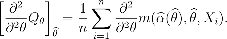
Under (C.8) and (C.9), the gradient vector and the Hessian matrix of Q_θ are

$$\frac{\partial }{\partial \theta }{Q}_{\theta }=\frac{1}{n}{\displaystyle \sum _{i=1}^n\frac{\partial }{\partial \theta }m(\stackrel{⌢}{\alpha }(\theta ),\theta ,X_i)}$$

(30)

$$\frac{{\partial }^2}{{\partial }^2\theta }{Q}_{\theta }=\frac{1}{n}{\displaystyle \sum _{i=1}^n\frac{{\partial }^2}{{\partial }^2\theta }m(\stackrel{⌢}{\alpha }(\theta ),\theta ,X_i)}.$$

(31)

Proof

Since

$$Q_{\theta }=\frac{1}{n}{\displaystyle \sum _{i=1}^{n}m(\stackrel{⌢}{\alpha }(\theta ),\theta ,X_i)}$$

(32)

derivation yields

(33)

Note that, by its very definition, $\stackrel{⌢}{\alpha }(\theta )$ is a solution of the equation

$$\frac{1}{n}{\displaystyle \sum _{i-1}^n\frac{\partial }{\partial \alpha }m(\alpha ,\theta ,X_i)=0}$$

(34)

taken with respect to α, therefore

$$\frac{\partial }{\partial \theta }{Q}_{\theta }=\frac{1}{n}{\displaystyle \sum _{i=1}^n\frac{\partial }{\partial \theta }m(\stackrel{⌢}{\alpha }(\theta ),\theta ,X_i).}$$

(35)

On the other hand,

(36)

$$=\frac{1}{n}{\displaystyle \sum _{i=1}^n\frac{{\partial }^2}{{\partial }^2\theta }m(\stackrel{⌢}{\alpha }(\theta ),\theta ,X_i).}$$

(37)

Proposition 3

Under conditions (C.1)–(C.3) and (C.8)–(C.9) and assuming that the integrals ${\displaystyle \int \left|\right|\frac{{\partial }^2}{{\partial }^2\theta }m({\theta }_0,{\theta }_0,x)\left|\right|}{f}_{{\theta }_0}(x)\mathrm{d}x$, ${\displaystyle \int \left|\right|\frac{{\partial }^3}{{\partial }^2\theta \partial \alpha }m({\theta }_0,{\theta }_0,x)\left|\right|}{f}_{{\theta }_0}(x)\mathrm{d}x$ and ${\displaystyle \int \left|\right|\frac{{\partial }^3}{{\partial }^3\theta }m({\theta }_0,{\theta }_0,x)\left|\right|}{f}_{{\theta }_0}(x)\mathrm{d}x$ are finite, the gradient vector and the Hessian matrix of Q_θ evaluated in $\theta =\stackrel{⌢}{\theta }$ satisfy

$${\left[\frac{\partial }{\partial \theta }{Q}_{\theta }\right]}_{\stackrel{⌢}{\theta }}=0$$

(38)

$${\left[\frac{{\partial }^2}{{\partial }^2\theta }{Q}_{\theta }\right]}_{\stackrel{⌢}{\theta }}=\ddot{\phi }(1)I({\theta }_0)+o_P(1).$$

(39)

Proof

By the very definition of $\stackrel{⌢}{\theta }$, the equality (38) is verified. For the second relation, we take $\theta =\stackrel{⌢}{\theta }$ in Equation (31) and obtain

(40)

A Taylor expansion of $\frac{1}{n}{\displaystyle {\sum }_{i=1}^n\frac{{\partial }^2}{{\partial }^2\theta }m(\alpha ,\theta ,X_i)}$ as function of (α, θ) around to (θ₀, θ₀) yields

Using the fact that ${\displaystyle \int \left|\right|\frac{{\partial }^2}{{\partial }^2\theta }m({\theta }_0,{\theta }_0,x)|{|}^2{f}_{{\theta }_0}(x)\mathrm{d}x}$ is finite, the weak law of large numbers leads to

(41)

Then, since $(\stackrel{⌢}{\alpha }(\stackrel{⌢}{\theta })-{\theta }_0)=o_P(1)$ and $(\stackrel{⌢}{\theta }-{\theta }_0)=o_P(1)$, and taking into account that ${\displaystyle \int \left|\right|\frac{{\partial }^3}{{\partial }^2\theta \partial \alpha }m({\theta }_0,{\theta }_0,x)\left|\right|f_{{\theta }_0}(x)\mathrm{d}x}$ and ${\displaystyle \int \left|\right|\frac{{\partial }^3}{{\partial }^3\theta }m({\theta }_0,{\theta }_0,x)\left|\right|f_{{\theta }_0}(x)\mathrm{d}x}$ are finite, we deduce that

(42)

Thus we obtain Equation (39).

In the following, we suppose that conditions of Proposition 1, Proposition 2 and Proposition 3 are all satisfied. These conditions allow obtaining an asymptotically unbiased estimator of the expected overall discrepancy.

Proposition 4

When the true model g belongs to the parametric model (f_θ), the expected overall discrepancy evaluated at $\stackrel{⌢}{\theta }$ is given by

$$E[W_{\widehat{\theta }}]=E[Q_{\widehat{\theta }}+\ddot{\phi }(1){(\widehat{\theta }-{\theta }_0)}^{t}I({\theta }_0)(\widehat{\theta }-{\theta }_0)+R_n],$$

(43)

where $R_n=o(||{\theta }_0-\stackrel{⌢}{\theta }|{|}^2)$.

Proof

A Taylor expansion of Q_θ around to $\stackrel{⌢}{\theta }$ yields

(44)

and using Proposition 3, we have

(45)

Taking θ = θ₀, for large n, it holds

(46)

and consequently

(47)

Where $R_n=o(||{\theta }_0-\stackrel{⌢}{\theta }|{|}^2)$.

According to Proposition 2 it holds

(48)

Note that

(49)

Then, combining Equation (48) with Equations (49) and (47), we get

(50)

Proposition 4 shows that an asymptotically unbiased estimator of the expected overall discrepancy is given by

$$Q_{\stackrel{⌢}{\theta }}+\ddot{\phi }(1){(\stackrel{⌢}{\theta }-{\theta }_0)}^{t}I({\theta }_0)(\stackrel{⌢}{\theta }-{\theta }_0).$$

(51)

According to Proposition 1, $\sqrt{n}(\stackrel{⌢}{\theta }-{\theta }_0)$ is asymptotically distributed as N_p (0, I (θ₀)⁻¹). Consequently, $n{(\stackrel{⌢}{\theta }-{\theta }_0)}^{t}I({\theta }_0)(\stackrel{⌢}{\theta }-{\theta }_0)$ has approximately a ${\mathrm{\chi }}_p^2$ distribution. Then, taking into account that $no(||\stackrel{⌢}{\theta }-{\theta }_0|{|}^2)=o_P(1)$, an asymptotically unbiased estimator of n-times the expected overall discrepancy evaluated at $\stackrel{⌢}{\theta }$ is provided by

$$n{Q}_{\stackrel{⌢}{\theta }}+\ddot{\phi }\partial (1)p.$$

(52)

3.3. Influence Functions

In the following, we compute the influence function of the statistics $Q_{\stackrel{⌢}{\theta }}$. As it is known, the influence function is a useful tool for describing the robustness of an estimator. Recall that a map T defined on a set of distribution functions and parameter space valued is a statistical functional corresponding to an estimator $\stackrel{⌢}{\theta }$ of the parameter θ, if $\stackrel{⌢}{\theta }=T(F_n)$, where F_n is the empirical distribution function associated to the sample. The influence function of T at f_θ is defined by

$$\text{IF(}x\text{; }T\text{, }{F}_{\theta }\text{):}{=\frac{\partial T({\tilde{F}}_{\epsilon x})}{\partial \epsilon }|}_{\epsilon =0}$$

(53)

where ${\tilde{F}}_{\epsilon x}:=(1-\epsilon )F_{\theta }+\epsilon {\delta }_x,\epsilon >0,{\delta }_x$ being the Dirac measure putting all mass at x. Whenever the influence function is bounded with respect to x, the corresponding estimator is called robust (see [31]).

Since

$$Q_{\stackrel{⌢}{\theta }}=\frac{1}{n}{\displaystyle \sum _{i=1}^{n}m(\stackrel{⌢}{\alpha }(\stackrel{⌢}{\theta }),\stackrel{⌢}{\theta },X_i),}$$

(54)

the statistical functional corresponding to $Q_{\stackrel{⌢}{\theta }}$, which we denote by U (•), is defined by

$$U(F):={\displaystyle \int m(T_{V(F)}(F),V(F),y)\mathrm{d}F(y)}$$

(55)

where t_θ(f) is the statistical functional associated to the estimator $\stackrel{⌢}{\alpha }(\theta )$ and V (F) is the statistical functional associated to the estimator $\stackrel{⌢}{\theta }$.

Proposition 5

The influence function of $Q_{\stackrel{⌢}{\theta }}$ is

$$\text{IF}(x;U,F_{{\theta }_0})=\ddot{\phi }(1)\frac{{\dot{f}}_{{\theta }_0}(x)}{f_{{\theta }_0}(x)}.$$

(56)

Proof

For the contaminated model ${\tilde{F}}_{\epsilon x}:=(1-\epsilon )F_{{\theta }_0}+\epsilon {\delta }_x$, it holds

(57)

Derivation with respect to ε yields

Note that m (θ₀, θ₀, y) = 0 for any y and ${\displaystyle \int \frac{\partial }{\partial \alpha }m({\theta }_0,{\theta }_0,y)\mathrm{d}{F}_{{\theta }_0}(y)=0}$. Also, some straightforward calculations give

$${\displaystyle \int \frac{\partial }{\partial \theta }m({\theta }_0,{\theta }_0,y)}\mathrm{d}{F}_{{\theta }_0}(y)=\ddot{\phi }(1)I({\theta }_0).$$

(58)

On the other hand, according to the results presented in [12], the influence function of the minimum dual divergence estimator is

$$\text{IF}(x;V,F_{{\theta }_0})=I{({\theta }_0)}^{-1}\frac{{\dot{f}}_{{\theta }_0}(x)}{f_{{\theta }_0}(x)}.$$

(59)

Consequently, we obtain Equation (60).

Note that, for Cressie–Read divergences, it holds

$$\text{IF}(x;U,F_{{\theta }_0})=\frac{{\dot{f}}_{{\theta }_0}(x)}{f_{{\theta }_0}(x)}$$

(60)

irrespective of the used divergence, since ${\ddot{\phi }}_{\mathrm{\gamma }}(1)=1$, for any γ.

Generally, $\text{IF}(x;U,F_{{\theta }_0})$ is not bounded, therefore the robustness of the statistics $Q_{\stackrel{⌢}{\theta }}$, as measured by the influence function, does not hold.

4. Conclusions

The dual representation of divergences and corresponding minimum dual divergence estimators are useful tools in statistical inference. The presented theoretical results show that, in the context of model selection, these tools provide asymptotically unbiased criteria. These criteria are not robust in the sense of the bounded influence function, but this fact does not exclude the stability of the criteria with respect to other robustness measures. The computation of $Q_{\stackrel{⌢}{\theta }}$ could lead to serious difficulties, for example when considering various regression models to choose from. Such difficulties are implied by the double optimization in the criterion. Therefore, from the computation point of view, some other existing model selection criteria could be preferred. On the other hand, some performant computation techniques, involving such a double optimization, could arrive in the favor of using these new criteria also. These problems represent the topic of future research.

References

- Pardo, L. Statistical Inference Based on Divergence Measures; Chapmann & Hall: Boca Raton, FL, USA, 2006. [Google Scholar]
- Basu, A.; Shioya, H.; Park, C. Statistical Inference: The Minimum Distance Approach; Chapmann & Hall: Boca Raton, FL, USA, 2011. [Google Scholar]
- Beran, R. Minimum Hellinger distance estimates for parametric models. Ann. Stat 1977, 5, 445–463. [Google Scholar]
- Tamura, R.N.; Boos, D.D. Minimum Hellinger distance estimation for multivariate location and covariance. J. Am. Stat. Assoc 1986, 81, 223–229. [Google Scholar]
- Simpson, D.G. Minimum Hellinger distance estimation for the analysis of count data. J. Am. Stat. Assoc 1987, 82, 802–807. [Google Scholar]
- Simpson, D.G. Hellinger deviance tests: Efficiency, breakdown points, and examples. J. Am. Stat. Assoc 1989, 84, 104–113. [Google Scholar]
- Toma, A. Minimum Hellinger distance estimators for multivariate distributions from Johnson system. J. Stat. Plan. Inference 2008, 183, 803–816. [Google Scholar]
- Lindsay, B.G. Efficiency versus robustness: The case of minimum Hellinger distance and related methods. Ann. Stat 1994, 22, 1081–1114. [Google Scholar]
- Basu, A.; Lindsay, B.G. Minimum disparity estimation for continuous models: Efficiency, distributions and robustness. Ann. Inst. Stat. Math 1994, 46, 683–705. [Google Scholar]
- Basu, A.; Harris, I.R.; Hjort, N.L.; Jones, M.C. Robust and efficient estimation by minimising a density power divergence. Biometrika 1998, 85, 549–559. [Google Scholar]
- Broniatowski, M.; Keziou, A. Parametric estimation and tests through divergences and duality technique. J. Multivar. Anal 2009, 100, 16–36. [Google Scholar]
- Toma, A.; Broniatowski, M. Dual divergence estimators and tests: Robustness results. J. Multivar. Anal 2011, 102, 20–36. [Google Scholar]
- Toma, A.; Leoni-Aubin, S. Robust tests based on dual divergence estimators and saddlepoint approximations. J. Multivar. Anal 2010, 101, 1143–1155. [Google Scholar]
- Mallows, C.L. Some comments on Cp. Technometrics 1973, 15, 661–675. [Google Scholar]
- Stone, M. Cross-validatory choice and assessment of statistical predictions. J. R. Stat. Soc. Ser. B 1974, 36, 111–147. [Google Scholar]
- Akaike, H. Information theory and an extension of the maximum likelihood principle, Proceedings of the Second International Symposium on Information Theory, Akademiai Kaido, Budapest, 1973; Petrov, B.N., Csaki, I.F., Eds.; pp. 267–281.
- Schwarz, G. Estimating the dimension of a model. Ann. Stat 1978, 6, 461–464. [Google Scholar]
- Konishi, S.; Kitagawa, G. Generalised information criteria in model selection. Biometrika 1996, 83, 875–890. [Google Scholar]
- Ronchetti, E. Robust model selection in regression. Stat. Probab. Lett 1985, 3, 21–23. [Google Scholar]
- Ronchetti, E.; Staudte, R.G. A robust version of Mallows’ CP. J. Am. Stat. Assoc 1994, 89, 550–559. [Google Scholar]
- Maronna, R.A.; Martin, R.D.; Yohai, V.J. Robust Statistics: Theory and Methods; Wiley: New York, NY, USA, 2006. [Google Scholar]
- Karagrigoriou, A.; Mattheou, K.; Vonta, F. On asymptotic properties of AIC variants with applications. Open J. Stat 2011, 1, 105–109. [Google Scholar]
- Mattheou, K.; Lee, S.; Karagrigoriou, A. A model selection criterion based on the BHHJ measure of divergence. J. Stat. Plan. Inference 2009, 139, 228–235. [Google Scholar]
- Cressie, N.; Read, T.R.C. Multinomial goodness of fit tests. J. R. Stat. Soc. Ser. B 1984, 46, 440–464. [Google Scholar]
- Ru¨schendorf, L. On the minimum discrimination information theorem. Stat. Decis 1984, 1, 163–283. [Google Scholar]
- Liese, F.; Vajda, I. Convex Statistical Distances; BSB Teubner: Leipzig, Germany, 1987. [Google Scholar]
- Toma, A.; Leoni-Aubin, S. Portfolio selection using minimum pseudodistance estimators. Econ. Comput. Econ. Cybern. Stud. Res 2013, 46, 117–132. [Google Scholar]
- Kallberg, D.; Leonenko, N.; Seleznjev, O. Statistical inference for Re´nyi entropy functionals. In Conceptual Modelling and Its Theoretical Foundations; Lecture Notes in Computer Science; Springer: Berlin/Heidelberg, Germany, 2012; Volume 7260, pp. 36–51. [Google Scholar]
- Preda, V.; Dedu, S.; Sheraz, M. New measure selection for Hunt-Devolder semi-Markov regime switching interest rate models. Physica A 2014, 407, 350–359. [Google Scholar]
- Liese, F.; Vajda, I. On divergences and informations in statistics and information theory. IEEE Trans. Inf. Theory 2006, 52, 4394–4412. [Google Scholar]
- Hampel, F.R.; Ronchetti, E.; Rousseeuw, P.J.; Stahel, W. Robust Statistics: The Approach Based on Influence Functions; Wiley: New York, NY, USA, 1986. [Google Scholar]
© 2014 by the authors; licensee MDPI, Basel, Switzerland This article is an open access article distributed under the terms and conditions of the Creative Commons Attribution license (http://creativecommons.org/licenses/by/3.0/).
Share and Cite
Toma, A. Model Selection Criteria Using Divergences. Entropy 2014, 16, 2686-2698. https://doi.org/10.3390/e16052686
Toma A. Model Selection Criteria Using Divergences. Entropy. 2014; 16(5):2686-2698. https://doi.org/10.3390/e16052686
Chicago/Turabian StyleToma, Aida. 2014. "Model Selection Criteria Using Divergences" Entropy 16, no. 5: 2686-2698. https://doi.org/10.3390/e16052686