Market Efficiency, Roughness and Long Memory in PSI20 Index Returns: Wavelet and Entropy Analysis

Abstract

In this study, features of the financial returns of the PSI20index, related to market efficiency, are captured using wavelet- and entropy-based techniques. This characterization includes the following points. First, the detection of long memory, associated with low frequencies, and a global measure of the time series: the Hurst exponent estimated by several methods, including wavelets. Second, the degree of roughness, or regularity variation, associated with the Hölder exponent, fractal dimension and estimation based on the multifractal spectrum. Finally, the degree of the unpredictability of the series, estimated by approximate entropy. These aspects may also be studied through the concepts of non-extensive entropy and distribution using, for instance, the Tsallis q-triplet. They allow one to study the existence of efficiency in the financial market. On the other hand, the study of local roughness is performed by considering wavelet leader-based entropy. In fact, the wavelet coefficients are computed from a multiresolution analysis, and the wavelet leaders are defined by the local suprema of these coefficients, near the point that we are considering. The resulting entropy is more accurate in that detection than the Hölder exponent. These procedures enhance the capacity to identify the occurrence of financial crashes.

1. Introduction

The purpose of this paper is to analyze two main issues concerning the Portuguese Index PSI20 daily returns, in the period from 2000 to 2013. The first issue is market efficiency (see Kristoufek and Vorvsda [1,2]). A market is called efficient if prices are adjusted so that they reflect the new information (see Fama [3] and Samuelson [4]). It is assumed that no investor can predict any information that is not already available in prices. As for the correlation structure of the series, there should be neither long memory nor local persistence or anti-persistence reflected in less rough or rougher paths, respectively. As a consequence, three aspects of the series are symptoms of efficiency: unpredictability, no long memory and the roughness of the series path (irregularity). These will be evaluated for the PSI20 series to check for the existence of deviations from efficiency.

Long memory reflects a tendency for a slow decay of the magnitude of the time series correlations as a function of lag size, but still preserving stationarity. In a strict sense, it is defined as reflecting a trend-like behavior, that is, persistence (positive long memory). In a broader sense, it may reflect either persistence or anti-persistence, that is, a switching behavior more pronounced than that of a random process (negative long memory); see [5]. Roughness is a time series feature that describes its tendency for an erratic behavior with frequent and heterogeneous changes.

While long memory, measured by the Hurst coefficient, H, is a global characteristic of the series, roughness, measured by the fractal dimension, D, is a local one. For a self-affine process, given by:

$$X(ct)=c^{H}X(t),$$

it is verified that D + H = 2 (see, for instance, [1]). In these processes, the global long memory characteristic of the series is a reflection of its local roughness characteristic.

A generalization is given by multifractal processes, given by:

$$E[X(t)]=c(q)t^{\tau (q)+1}$$

where τ (q) is a concave function. In a monofractal process, we have:

$$\tau (q)+1=Hq,$$

so that a linear scaling is attained.

The definition of entropy as a measure of uncertainty, or lack of information, is used not only to measure unpredictability, but also to reflect indirectly the degree of roughness in the path of the series.

As an alternative in the analysis of market efficiency, we will use the concept of the q-triplet, created by Tsallis [6] in the context of nonextensive statistical mechanics. It is used for the characterization of non-integrable dynamical systems, where all Lyapunov coefficients vanish. It consists of a threefold determination of an entropic coefficient, q, in the context of: (1) the sensitivity to initial conditions in a dynamical system, which may be seen as reflecting unpredictability; (2) relaxation of macroscopic variable towards a stationary state, which in a time series, may be taken to detect the existence of long memory; (3) the stationary distribution obtained after the constrained optimization of an entropy function, where the departure of this distribution from the Gaussian distribution is the result of self-organization in the market leading to a rougher path. For several empirical approaches, see Pavlos et al. [7], Ferri et al. [8], de Freitas et al. [9], De Sousa and Rostirolla [10] and, in the finance area, Queirós et al. [11].

The second issue is local regularity, which is related to the identification of crisis events. Financial time series evolve showing patterns, such as time varying volatility and abrupt changes. Irregularity presented by a signal gives information about its behavior. The characterization of irregularity is given by the quantification of the local regularity of a function, f. The pointwise Hölder exponent is one of the quantifiers proposed to measure the local regularity; in fact, a low pointwise Hölder exponent reflects a highly irregular path around the point, whereas a high pointwise Hölder exponent is related to a smooth behavior. Jaffard [12] proposed a characterization of the local regularity using the wavelet coefficients obtained from the wavelet decomposition of the signal; see also [13]. Rosenblatt et al. [14] studied the local regularity of a time series applying an entropy measure based on the wavelet leaders.

The rest of this paper is organized as follows. In Section 2, we present the methods for studying market efficiency, using the concepts of long memory, unpredictability and path roughness (Section 2.1) and the concept of q-triplet (Section 2.2). The treatment of the wavelet approach for measuring irregularity is given in Section 3. Results are presented in Section 4. We provide a brief conclusion in Section 5.

2. Market Efficiency

Analysis of the existence of efficiency in the financial markets is an important issue in financial analysis. A capital market is considered efficient if prices, at each moment, reflect all relevant information. Three types of efficiency are considered according to the degree of information incorporated: weak efficiency if information includes only past prices; semi-strong efficiency if information includes also the information publicly available in the market; and strong efficiency if it includes all information, public or private.

2.1. Three Markers for Market Efficiency

We analyze three aspects of the return series, which result from the existence of efficiency. The empirical testing of those aspects correspond to the check for the existence of efficiency.

The assurance of efficiency in the market is attained by an automatic elimination of arbitrage opportunities. The absence of arbitrage implies that there will be no long memory, described as a power decay of correlations, in the return series—the first aspect that characterizes the return series. As a consequence of the absence of arbitrage opportunities, it is expected that the price series are modeled as a martingale and the corresponding returns as a martingale difference that is unpredictable—the second aspect of the return series. This implies an erratic behavior of prices, which is quantified as a high degree of roughness—the third aspect of the return series.

2.1.1. Long Memory

A long memory process was originally defined and motivated, respectively, by McLeod and Hipel [15] and Hall [16], as a stationary process for which autocorrelations absolute values are not summable in the discrete case, that is:

$${\displaystyle \sum _{h=-\infty }^{+\infty }\left|\rho (h)\right|=+\infty ,}$$

(1)

where ρ(h) is the lag, h, autocorrelation.

In what follows, we assume that the parameter, H, verifies $\frac{1}{2}<H<1$. The restriction H < 1 assures that the process is stationary. Additionally, imposing $H>\frac{1}{2}$ assures that the process is persistent (for $H=\frac{1}{2}$, there is short memory, while for $0<H<\frac{1}{2}$, there is long memory, although negative; see [5]). We retain the case of positive long memory, which is the one usually observed in the financial time series representing volatility.

An alternative definition of a long memory process is attained by the asymptotic characterization of autocorrelations (see [17]):

$$\rho (h)\sim h^{2H-2}{\ell }_1(h)\text{as}h\to +\infty ,$$

(2)

where ℓ₁ is a slow variation function (that is, a measurable function, which is positive in a neighborhood of ∞ and for which: $\forall c>0\frac{f(cx)}{f(x)}\to 1$ as x → +∞), and H is called the Hurst coefficient. We can see that the autocorrelation function has a slow decay, as a power law function. In the discrete case, this implies the non-summability of autocorrelations.

A third alternative definition may be stated in the frequency domain; see [18]:

$$f(\mathrm{\lambda })\sim {\mathrm{\lambda }}^{1-2H}{\ell }_2\left(\frac{1}{\left|\mathrm{\lambda }\right|}\right)\text{as}\mathrm{\lambda }\to 0.$$

(3)

where ℓ₂ is a slow variation function, λ denotes a frequency and f is the spectral density. Therefore, the spectral density tends to infinity as the frequency approaches zero.

Remark 1

(i) There is no equivalence between this and the precedent definition, but it is implied by it if ℓ₁ is almost monotone, that is:

$$\exists \alpha >0{\displaystyle {\int }_0^x{t}^{\alpha }\left|d{\ell }_1(t)\right|=O(x^{\alpha }{\ell }_1(x)),x\to +\infty .}$$

(4)

A last definition of a discrete time long memory process, {yt}, based on Wold’s decomposition:

$$y_t=u+{\displaystyle \sum _{k=0}^{+\infty }{\Psi }_k{\epsilon }_{t-k},}$$

(5)

where${\Psi }_0=1,{\displaystyle \sum _{k=1}^{+\infty }{({\Psi }_k)}^2<+\infty }$ and {ε_t} is a white noise, states that:

$${\Psi }_j\sim j^{H-\frac{3}{2}}{\ell }_3(j),$$

(6)

ℓ₃ being a slow variation function.

(ii) Condition (6) implies (2).

(iii) If$H=\frac{1}{2}$, we have a short memory process; if H ≥ 1, the process is non-stationary. Therefore, the long memory case is an intermediate case between these two. For$H\le \frac{1}{2}$, we have an antipersistent behavior.

(iv) Long memory is characterized by a power law asymptotic behavior, where the Hurst coefficient plays a prominent role.

In alternative definitions of long memory, we consider asymptotic relations based on power functions, either in the time or in the frequency domain. By applying a logarithm transformation on the variables, we obtain linear regressions, which may be fitted by a least squares approach. This is the mechanism taken to build several estimation methods for the Hurst coefficient, H.

Considering a long memory process in the form $y_t=u+{\epsilon }_t{(1-L)}^{-H+\frac{1}{2}}$, we have $f_y(\mathrm{\lambda })={\left[4{\sin }^2\left(\frac{\mathrm{\lambda }}{2}\right)\right]}^{-H\frac{\mathrm{\lambda }}{2}}{f}_{\epsilon }(\mathrm{\lambda })$, where {ε_t} is a white noise, u = E(y_t), λ denotes a frequency and L is the lag operator. Taking logarithms: $\ln f_y(\mathrm{\lambda })=\ln f_{\epsilon }(\mathrm{\lambda })-\left(H-\frac{\mathrm{\lambda }}{2}\right)\left[4{\sin }^2\left(\frac{\mathrm{\lambda }}{2}\right)\right]$. Therefore, we have the linear regression:

$$\ln {\widehat{f}}_y({\mathrm{\lambda }}_k)=\beta -(H-\frac{\mathrm{\lambda }}{2})\ln [4{\sin }^2\left(\frac{{\mathrm{\lambda }}_k}{2}\right)]+{\epsilon }_k,k=1,2,\dots ,{\eta }_f(T)$$

(7)

where β = ln f_ε(λ) and η_f (T) is the number of frequencies considered. This is the regression used to obtain the Geweke and Porter–Hudak estimator [19].

The periodogram estimator is obtained after (3), which allows one to obtain a linear regression of $\ln {\widehat{f}}_y$ on ln λ, for frequencies λ near zero, with the slope given by 1 – 2H.

The R/S (range over standard deviation) statistic, originally proposed by Hurst [20], is given by:

$$Q_T=\frac{1}{S_T}\left[\underset{1\le k\le T}{max}{\displaystyle \sum _{j=1}^k(y_t-\overline{y})-}\underset{1\le k\le T}{min}{\displaystyle \sum _{j=1}^k(y_j-\overline{y})}\right],$$

(8)

where $\overline{y}$ and S_T are, respectively, the sample mean and the sample standard deviation. This is an increasing measure of long memory, and for i.i.d. Gaussian random variables, yt, we have:

$$\frac{Q_T}{\sqrt{T}}\Rightarrow V=V_s-V_{s-1},$$

(9)

where {V_t} is a Brownian bridge and “⇒” stands for weak convergence. Lo [17] proposed a more robust version, which assures the convergence for short memory processes; here, S_T is substituted by the long run Newey–West standard deviation [21]. Estimation based on the R/S statistic is obtained after a linear regression of ln Q_T on ln T, where T is the size of the subsamples used to estimate the R/S statistic. This regression has slope H.

Other approaches may be taken, for instance, the Whittle estimator [22] is obtained by maximum likelihood on the frequency domain, considering frequencies near zero.

2.1.2. Fractal Dimension

The fractal dimension is a measure of roughness, and in opposition to the Long memory characterization, it measures the local memory of the series (Kristoufek and Vorvsda [1]). When modeling the dynamic behavior of a variable, by the solution of deterministic equations, the set of all instantaneous states of the system is the phase space. The subset of the phase space towards which the system converges, called the attractor, may be a fractal (Theiler [23]). A fractal is an irregular geometric form, the patterns of evolution being similar at different time scales (self-similar). In this context, the fractal dimension of an attractor measures the number of degrees of freedom of the system. When the self-similarity of the geometric form through scales is not perfect, it is called statistical. The fractal dimension can be obtained as an exponent of a scaling behavior of a quantity, measuring the bulk of an object (here, bulk may correspond to the mass of the object) with respect to another measuring the corresponding size (linear distance):

$$\text{bulk}\sim {\text{size}}^{\text{dimension}}$$

(see Theiler [23]) from which we obtain:

$$\ln \left(\text{bulk}\right)\sim dimension\times \ln \left(\text{size}\right),$$

so that the dimension is given by:

$$\underset{\text{size}\to 0}{\lim }\frac{ln(\text{bulk})}{ln(\text{size})}.$$

(10)

This is a local quantity from which a global definition of the fractal dimension can be found by averaging.

(1) The classical box-counting dimension is defined as follows. We take a partition of the state space in a grid where each box has size ε. Then, count the non-empty boxes (that is, those containing points attained by the attractor). The scaling of this counting number, N(ε), with respect to size ε leads to dimension: $D_f=\underset{\epsilon \to 0}{\lim }\frac{ln(\frac{1}{N(\epsilon )})}{ln\epsilon }$; which is an upper bound of the Hausdorff dimension (under weak regularity conditions, they coincide). This definition is global, since the bulk, $\frac{1}{N(\epsilon )}$, is the average proportion that each non-empty box has of the whole fractal.

(2) The Hall–Wood estimator is a version of the box-counting estimator, this being obtained from (10) (see Gneiting et al. [37]). In fact, considering the boxes of size (scale) ε that intersect with the linearly interpolated data graph $\{(t,X_t):t=\frac{i}{n},i=0,1,\dots ,n\}$, there are N (ε) such boxes with a total area of A(ε) ∝ N(ε)ε². Therefore, the dimension is given by:

$$\begin{array}{l}D=-{\lim }_{\epsilon \to 0}\frac{\ln N(\epsilon )}{\ln \epsilon }\\ \propto -{\lim }_{\epsilon \to 0}\frac{\ln \frac{A(\epsilon )}{{\epsilon }^2}}{\ln \epsilon }\\ =2-{\lim }_{\epsilon \to 0}\frac{\ln A(\epsilon )}{\ln \epsilon }.\end{array}$$

(11)

The Hall–Wood estimator is based on an ordinary least squares regression fit of $\ln \widehat{A}(\frac{\ell }{n})$ on $\ln \frac{\ell }{n}$:

$${\widehat{D}}_{HW}=2-\frac{{\displaystyle \sum _{\ell =1}^L(s_{\ell }-\overline{s})\ln \widehat{A}(\frac{\ell }{n})}}{{\displaystyle {\sum }_{\ell =1}^L{(s_{\ell }-\overline{s})}^2}},$$

(12)

where n + 1 is the number of observations and ℓ takes the values 2^k, k = 0, 1,…, K being K = ln₂(n). $\widehat{A}\left(\frac{\ell }{n}\right)$ is an estimator of $A\left(\frac{\ell }{n}\right)$ at scale ${\epsilon }_{\ell }=\frac{\ell }{n}(\ell =1,2,\dots )$ given by:

$$\widehat{A}(\frac{\ell }{n})=\frac{{\displaystyle {\sum }_{\ell =1}^{\lfloor \frac{n}{\ell }\rfloor }|X_{i\frac{\ell }{n}}-X_{(i-1)\frac{\ell }{n}}|}}{\frac{n}{\ell }}$$

and $\lfloor \frac{n}{\ell }\rfloor$ denotes the greatest integer smaller or equal to $\frac{n}{\ell },\overline{s}=\frac{{\displaystyle {\sum }_{\ell =1}^L{s}_{\ell }}}{L}$ and $s_{\ell }=\ln \left(\frac{\ell }{n}\right),L\ge 2$. It is recommended that L = 2, so that bias is minimized:

$${\widehat{D}}_{HW}=2-\frac{\ln \widehat{A}(\frac{2}{n})-\ln \widehat{A}(\frac{1}{n})}{\ln 2}$$

(13)

(see Hall et al. [24]).

(3) The Genton estimator is based on the variogram given by 2γ₂ (t) where:

$${\mathrm{\gamma }}_2(t)=\frac{1}{2}E[{(X_u-X_{u+t})}^2].$$

(14)

for which we have γ₂(t) ∝ |ct|^α, as t → 0. The graph of a sample path has the fractal dimension given by $D=d+1-\frac{\alpha }{2}$, where d is the dimension of the considered random vector. When we study a single random variable, we have d = 1, so that:

$$D=2-\frac{\alpha }{2}.$$

(15)

The ordinary least squares regression fit of:

$${\widehat{V}}_2(\frac{\ell }{n})=\frac{1}{2}\frac{{\displaystyle \sum _{i=1}^n{(X_{\frac{i}{n}}-X_{\frac{i-\ell }{n}})}^2}}{n-\ell }$$

on $\ln \left(\frac{\ell }{n}\right)$ leads to the following estimator for α:

$$\widehat{\alpha }=\frac{{\displaystyle \sum _{\ell =1}^L(s_{\ell }-\overline{s})\ln {\widehat{V}}_2(\frac{\ell }{n})}}{{\displaystyle {\sum }_{\ell =1}^L{(s_{\ell }-\widehat{s})}^2}}.$$

(16)

Remark that ℓ, L, s_ℓ and $\overline{s}$ are defined as in (12). Substituting (16) into (15), we obtain the variogram estimator for the fractal dimension:

$${\widehat{D}}_{V,2}=2-\frac{1}{2}\frac{{\displaystyle \sum _{\ell =1}^L(s_{\ell }-\overline{s})}\ln {\widehat{V}}_2(\frac{\ell }{n})}{{\displaystyle {\sum }_{\ell =1}^L{(s_{\ell }-\widehat{s})}^2}}.$$

(17)

The mean squared error of the estimator is minimized for L = 2, so the following estimator is chosen:

$${\widehat{D}}_{V,2}=2-\frac{1}{2}\frac{\ln {\widehat{V}}_2(\frac{2}{n})-\ln {\widehat{V}}_2(\frac{1}{n})}{\ln 2}.$$

(18)

When the method of moments estimator ${\widehat{V}}_2\left(\frac{\ell }{n}\right)$ is replaced by the highly robust variogram estimator proposed by Genton [25], we have the Genton estimator for the ${\mathrm{\gamma }}_2(h),{\widehat{\text{γ}}}_2(h)=(\frac{Q_{N_h}^2}{2}),(h\in {\Re }^d)$, where:

$$\begin{array}{c}{Q}_{N_h}=2.2191{\left\{\right|V_i(h)-V_j(h)|;i\le j\}}_{(k)},\\ k=\left(\begin{array}{c}\lfloor \frac{N_h}{2}\rfloor +1\\ 2\end{array}\right)\end{array}$$

which is approximately equal to $\frac{1}{4}$ for large N_h, V (h) = X (t + h) − X (t), N_h is the number of points (x_i,x_j), such that {(x_i,x_j) : x_i – x_j = h}, and {⋅}(k) denotes the k-th quantile of the quantity inside the brackets.

2.1.3. Approximate Entropy (ApEn)

As Kristoufek and Vosvrda [1] state, entropy can be seen as measuring the complexity of the system, so that the greater the entropy, the greater the randomness. Approximate entropy was introduced by Pincus [26]. First, we consider a time series u (1),…, u (N) of observations equally spaced in time. Then, we fix the parameters, m and r, where m (integer) is the length of runs of data considered and r is an upper threshold for a distance defined below. A sequence:

$$x(1),\dots ,x(N-m+1)$$

is built by making x (i) = [u (i),…, u (i + m − 1)]. Then, approximate entropy (ApEn) is defined as:

$$\text{ApEn}={\mathrm{\Phi }}^m(r)-{\mathrm{\Phi }}^{m+1}(r)$$

(19)

where:

$${\mathrm{\Phi }}^m(r)=\frac{{\displaystyle \sum _{i=1}^{N-m+1}\ln C_i^m(r)}}{N-m+1}$$

(20)

being:

$$C_i^m(r)=\frac{number\{x(j):d[x(i),x(j)]\le r,1\le i,j\le N+m+1,j\ne i\}}{N-m+1}$$

(21)

and d a distance between x and x , given by:

$$d[x(i),x(j)]=ma{x}_{k=1,2,\dots ,n}(|u(i+k-1)-u(j+k-1)|).$$

As referred to by Pincus et al. [27], a heuristic interpretation of ApEn is that it measures the logarithm likelihood that runs of patterns that are close for m observations remain close on the next incremental comparisons. Note that ApEn may be written as:

$$\frac{{\displaystyle \sum _{i=1}^{N-m}\ln }\left(\frac{C_{N-m+1}^m(r)}{C_i^m(r)}\right)}{(N-m+1)(N-m)}.$$

(22)

Typically, it is chosen m = 2 or m = 3 (these values aim to obtain a good estimation for the conditional probability measured by the ApEn), the number of input data points, N, between 10^m and 30^m, and the parameter, r, depends on the application (see [27]).

Remark 2

This entropy is related to the more abstract Kolmogorov–Sinai entropy, given by:

$$\underset{r\to 0}{\lim }\underset{m\to \infty }{\lim }\underset{N\to +\infty }{\lim }[{\mathrm{\Phi }}^m(r)-{\mathrm{\Phi }}^{m+1}(r)].$$

(23)

Remark 3

Pincus and Kalman [28] point out that the irregularity or unpredictability of the time series is another way by which it may deviate from constancy, as an alternative to volatility, which refers to the magnitude of variations from observation to observation.

2.2. q-Triplet

The concept of the q-triplet created by Tsallis [6] arose in the context of nonextensive statistical mechanics for the characterization of non-integrable dynamical systems, where all Lyapunov coefficients vanish, concerning: (i) sensitivity to initial conditions; (ii) relaxation of macroscopic variable towards an anomalous stationary state; and (iii) the stationary distribution obtained after the constrained optimization of an entropy function. These three aspects lead to a threefold determination of the entropic coefficient, q, and are related to the three aspects of efficiency referred to before, respectively: (i) unpredictability; (ii) long memory; and (iii) roughness.

2.2.1. q-Sens

This indicator allows one to stress the power-law sensitivity to initial conditions (Lyra and Tsallis [29]). This sensitivity represents the deviation of two initially nearby paths:

$$\xi (t)=\underset{\mathrm{\Delta }x(0)\to 0}{\lim }\frac{\mathrm{\Delta }x(t)}{\mathrm{\Delta }x(0)}.$$

In the exponential deviation case, we have, ξ (t) ~ e^λ1t, where λ₁ is the Liapunov exponent. The power-law sensitivity to initial conditions is given by:

$$\xi (t)={[1+(1-q){\mathrm{\lambda }}_q(t)]}^{\frac{1}{1-q}},q\in \Re .$$

(24)

It is a generalization of the classical exponential case; the limit case as q → 1 recovers the exponential sensitivity. The expression for ξ (t) is the solution of $\frac{d\xi }{dt}={\mathrm{\lambda }}_q{\xi }^q$, while, in the exponential case, it is the solution of $\frac{d\xi }{dt}={\mathrm{\lambda }}_1\xi$.

The entropic index, q, is expressed as a function of the fractal scaling properties of the attractor. These properties are expressed through the multifractal formalism. In this context, we take for each scale a partition of the attractor with N boxes for which a probability measure is defined (p_i is the probability attributed to box i, given by the proportion of points of the path in box i). As N → ∞, we have, for a generic $\overline{q}$, a subset of boxes visited by the trajectory (at least once) for which: the number of such boxes, $N_{\overline{q}}$, scales as $N_{\overline{q}}\propto N^{f(\overline{q})}$; the partition function, ${\mathrm{\chi }}_{\overline{q}}(N)={\displaystyle \sum _{i=1}^N{p}_i^{\overline{q}}}$, scales as ${\mathrm{\chi }}_{\overline{q}}(N)\propto N^{-\tau (\overline{q})}$; the content of each box is roughly constant and scales as $p_{\overline{q}}\propto N^{-\alpha (\overline{q})}$. Note that $\alpha (\overline{q})$ is the local Hölder exponent in the scaling relation between the probability, $p_{\overline{q}}$, and the size of the box. Then, we have:

$${\mathrm{\chi }}_{\overline{q}}(N)={\displaystyle \sum _{i=1}^{N\overline{q}}{p}_i^{\overline{q}}\simeq N_{\overline{q}}{p}^{\overline{q}}\propto N^{f(\overline{q})-\overline{q}\alpha (\overline{q})}}$$

(25)

so that $N^{-\tau (\overline{q})}=N^{f(\overline{q})-\overline{q}\alpha (\overline{q})}$, and we obtain the Legendre transformation:

$$\text{τ(}\overline{q}\text{)}=\overline{q}\alpha (\overline{q})-f(\overline{q}).$$

(26)

Considering $f^{*}(\alpha (\overline{q}))=f(\overline{q})$, f  is defined as the multifractal spectrum, i.e., the fractal dimension of the subset of the boxes with Holder coefficient α, that is the subset of boxes whose number scales with N as N ^f (α). Note that τ (q) is equal to $(q-1)D_q^{*}$, where $D_q^{*}$ is the generalized fractal dimension of Renyi; see [23]:

$$\frac{1}{q-1}\underset{\epsilon \to 0}{\lim }\frac{\ln {\displaystyle {\sum }_i{p}_i^q}}{\ln \epsilon },$$

(27)

and ε is the scale.

We take the α values at the end points of the multifractal spectrum: ${\alpha }_{min}=\alpha (\overline{q}=+\infty )$ (resp. ${\alpha }_{max}=\alpha \left(\overline{q}=-\infty \right)$)) is associated with the most concentrated (resp. rarefied) region of the set. Our goal is to measure the power-law divergence of nearby orbits. Let B be the number of time steps over which the set of points in the attractor are generated. The measure on the i-box is roughly $\frac{1}{B}$, and the typical size of a box in the most concentrated (resp. rarefied) regions in the attractor is ℓ_+∞ (resp. ℓ_−∞). Note that for a given $\overline{q}$, we have p = B⁻¹. Then, recalling that α is the exponent in the scaling relation between the probability of a cell and its size, we have:

$$\ell \propto B^{-\frac{1}{\alpha }},$$

(28)

and consequently:

$$\ell \propto B^{-\frac{1}{\alpha }}=e^{-\frac{1}{\alpha }\ln B}.$$

(29)

Therefore, $\ln \ell \propto -\frac{\ln B}{\alpha }$. Taking into account that the smallest splitting between two nearby orbits is of order ℓ_+∞, and it can become at most a splitting of order ℓ_−∞, we can express (24) as:

$$\frac{{\ell }_{-\infty }}{{\ell }_{+\infty }}\propto B^{\frac{1}{1-q}}.$$

On the other hand, after (28), we have:

$$\frac{{\ell }_{-\infty }}{{\ell }_{+\infty }}\propto B^{\frac{1}{{\alpha }_{min}}-\frac{1}{{\alpha }_{max}}}.$$

(30)

Finally, $\frac{1}{1-q}=\frac{1}{{\alpha }_{min}}-\frac{1}{{\alpha }_{max}}$, which is the relation that allows one to obtain q_sens after the multifractal spectrum. The power-law sensitivity to initial conditions may be seen as a mechanism generating a certain degree of uncertainty, associated with the divergence of nearby orbits.

2.2.2. q-Rel

This indicator is defined in the context of the relaxation of an observable variable, Z_t, towards a stationary state. The variable, Ω(t), is defined as:

$$\Omega (t)=\frac{Z(t)-Z(\infty )}{Z(0)-Z(\infty )}$$

(31)

which behaves as a function of time t:

$$\Omega (\tau )\simeq e_{q_{rel}}^{-b\tau },$$

where $e_q^x$ is the q-exponential function given by $e_q^x={[1+(1-q)x]}^{\frac{1}{1-q}}$. Then,

$${\ln }_q\Omega (\tau )\simeq -b\tau ,$$

where ${\ln }_{q}x=\frac{x^{1-q}-1}{1-q}$ is the inverse function of $e_q^x$.

In a time series context, the relaxation variable is the autocorrelation function of Z given by:

$$C(\tau )=\frac{E[(Z(t)-E(Z(t)))(Z(t+\tau )-E(Z(t+\tau )))]}{E[{(Z(t+\tau )-E(Z(t+\tau )))}^2]}.$$

(32)

To estimate q_rel, we fit the regressions of ln_q C(τ) on τ, for each of the values of q in the interval [1, 1.5] with δ_q = 0.01, and choose the q-value for which the corresponding coefficient of determination is maximized (see Ferri et al. [8]; Pavlos et al. [7]). A high value for q_rel is a symptom of long-range memory.

2.2.3. q-Stat

This is the q parameter associated with a probability distribution, which arises by maximizing the Tsallis entropy $S_q=k\frac{1-{\displaystyle \int {[P(x)]}^{q}dx}}{q-1}$ (continuous version) under some adequate constraints (see Tsallis [6]). In the original context, considered by Tsallis (continuous version), these constraints are:

$${\displaystyle \int P(x)dx=1}$$

(33)

(the normalizing condition, so that we have a probability distribution) and:

$$E_q(x)={\displaystyle \int x\frac{{[P(x)]}^q}{{\displaystyle \int {[P(y)]}^{q}dy}}dx={\overline{\mu }}_q}$$

(34)

(the mean value under the escort distribution $\frac{{[P(x)]}^q}{{\displaystyle \int {[P(x)]}^q}}=P_q(x)$ is known to be ${\overline{\mu }}_q$). In this case, a q-exponential distribution is obtained; it is a generalization of the standard exponential distribution, which arises when we make q → 1.

In the financial context (see Queirós et al. [11]), it makes sense to add a constraint concerning the variance under P_q (x):

$$E_q[{(X-E_q(x))}^2]={\displaystyle \int {(x-{\overline{\mu }}_q)}^2\frac{{[P(x)]}^q}{{\displaystyle \int {[P(x)]}^q}}dx={\overline{\sigma }}_q^2.}$$

(35)

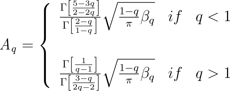
In this case, we attain the q-Gaussian distribution, with density function:

$$P(x)=A_q{[1+(q-1){\beta }_q{(x-{\overline{\mu }}_q)}^2]}^{\frac{1}{1-q}}(q<3),$$

(36)

where:

(37)

and ${\beta }_q={[(3-q){\overline{\sigma }}_q^2]}^{-1}$. In the limit case, q → 1, we have the standard Gaussian distribution.

Remark 4

When maximizing the classical Boltzmann–Gibbs–Shannon entropy, we obtain the Gaussian distribution.

Remark 5

In the context of information theory, the entropy measures the uncertainty associated with the variable, X (see Daroneeh et al. [30]). The Tsallis entropy, which is given, in the discrete case, by:

$$S_q=k\frac{1-{\displaystyle {\sum }_{i=1}^N{P}_i^q}}{q-1},$$

is nonextensive, that is, it does not, in general, verify the additivity axiom:

$$S(P\ast Q)=S(P)+S(Q),$$

where P and Q are probability distributions P ∗ Q: p_i ∗ q_j, i = 1…, m, k = 1,…, m. This relation is verified in the classical Boltzmann–Gibbs–Shannon entropy:

$$S=-{\displaystyle \sum _{i=1}^w{p}_i\ln p_i,}$$

the limiting case of S_q as q → 1.

In the general case, (q ≠ 1), we have:

$$S_q(P\ast Q)=S_q(P)+S_q(Q)+(1-q)S_q(P)S_q(Q).$$

Darooneh et al. [30] interpret this nonextensive case as reflecting the incompleteness of our knowledge represented by the escort distribution given by:$\frac{P_i^q}{{\displaystyle {\sum }_{i=1}^N{P}_i^q}}$.

Remark 6

Queirós et al. [11] refer to the fact that returns r follow a q-Gaussian law if its underlying dynamics are represented by the stochastic differential equation:

$$dr=-krdt+\sqrt{\theta {[p(r,t)]}^{1-q}}d{W}_t$$

(38)

where W_t is a Wiener process and p(r,t) the probability density function of r. The deterministic term reflects a mean-reversion mechanism, while the stochastic term reflects, for q > 1, the inverse relation between volatility and the density of the returns, so that the occurrence of rare returns (with high magnitude) causes higher instabilities in the market.

By reparametrization, it can be seen that the q-Gaussian distribution is, in fact, a t-student distribution where, n being the (non-integer) degrees of freedom:

$$-\frac{n+1}{2}=\frac{1}{1-q}\iff q=\frac{n+3}{n+1}.$$

Parameters can be estimated by maximum likelihood or minimizing the mean square deviation between this distribution and the empirical distribution (see Cortines et al. [31]).

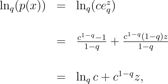
Alternatively, the following procedure may be applied. The range of values for X is subdivided into small cells of width δx centered at x_i, and we find the relative frequency of each cell. We estimate the probability distribution for x, p(x_i) through the properly normalized histogram. For 1 < q < 3, we rewrite p (x) as $G_q({\beta }_q,x-{\overline{\mu }}_q)=\frac{\sqrt{{\beta }_q}}{C_q}{e}_q{}^{-{\beta }_q{(x-{\overline{\mu }}_q)}^2}$, where $C_q=\frac{\sqrt{\mathrm{\pi }\Gamma }\left(\frac{3-q}{2q-2}\right)}{\sqrt{q-1\Gamma }\left(\frac{1}{q-1}\right)}$ and $e_q^x={[1+(1-q)x]}^{\frac{1}{1-q}}$.

Therefore, we have or $c=\frac{\sqrt{{\beta }_q}}{C_q}$ and $z=-{\beta }_q{(x-{\overline{\mu }}_q)}^2$.

(39)

where ln_q$(x)=\frac{x^q-1}{1-q}$. Taking a grid of values for q, with δ_q = 0.01 for q ∈ [1, 1.5], we obtain the best linear fit of ln_q (p(x)) over ${(x-\overline{x})}^2$ (that is, the one with a higher coefficient of determination). Then, we select the β-value, which minimizes ${\displaystyle \sum _i{(G_{q_{stat}}({\beta }_q,x_i)-p(x_i))}^2}$.

The q-Gaussian distribution may be seen as the one associated with a stationary state. The q-statcoefficient reflects the sensibility of the volatility to the occurrence of higher variations, such as crashes, resulting from self-organization in the market (see Pavlos et al. [7] and Ferri et al. [8]).

Remark 7

sde (38) expresses a mechanism to explain the clustering of high volatility based on a leverage effect, which may be linked to the fat tails of the q-exponential distribution. On the other hand, underlying this mechanism is the idea that markets have some self-organization, which causes a “roughness” on the financial time series.

3. Wavelets

A wavelet transform is a possible representation for a time series, so that the information given by the data can be captured in a clarified way. In order to capture the features of the time series, a basic function, called the mother wavelet, is used. The mother wavelet is shifted and stretched, so that the different frequencies, at different times, can be revealed and the events that are local in time are captured. This enables the wavelet transform to study nonstationary time series.

Wavelets can be used to decompose a time series showing its different components. The analysis using wavelets converts the original signal into different domains with different levels of resolution, so that the time series can be analyzed and processed. In fact, while Fourier transforms decompose the signal as a linear combination of sine and cosine functions, the wavelet transform explains the signal as a sum of flexible functions that allow a localization in frequency and time. Depending on the purposes of the study, we have different wavelet transforms: continuous and discrete. In particular, the discrete wavelet transform (DWT) allows one to decompose a time series, originating a set of coefficients that are obtained using the shifted and stretched versions of the mother wavelet. The DWT of a time series can be a way to represent a signal using a small number of terms. General references on wavelet transforms include, among others, [32–36].

The multiresolution pyramidal decomposition allows one to decompose a signal into detailed and approximated signals. The detailed signals express the high frequency components, while the approximated signals express the low frequency components. In order to check for the regularity, we should consider an orthogonal decimated discrete wavelet transform with fast decay derivatives and an appropriate number of vanishing moments.

In order to quantify the local regularity of a function, f, we can use, among others, the pointwise Holder exponent. If we have a low pointwise Holder exponent, it means that there is high irregularity; on the other hand, a high Hölder exponent is related to the smooth behavior of the function.

Jaffard [12] proposed a new way to characterize the regularity variation of f through the local suprema of the wavelet coefficients; this information is summarized in the wavelet leaders coefficients.

Consider Ψ₀, a real valued function with compact support and:

$${\displaystyle {\int }_{-\infty }^{+\infty }{\Psi }_0(t)dt=0.}$$

(40)

Define the number N ≥ 1, such that:

(1)

${\displaystyle \int t^k{\Psi }_0(t)dt=0,\forall k=0,1,2,\dots ,N-1}$

(2)

${\displaystyle \int t^N{\Psi }_0(t)dt\ne 0,}$

N is the number of vanishing moments of Ψ₀.

Let us consider translations and dilations of Ψ₀ :

$$\begin{array}{cc}{\Psi }_{j,k}(t)=2^{-j}{\Psi }_0(2^{-j}t-k),& j\in \end{array}\mathbb{N},k\in \mathbb{N}.$$

(41)

The set {Ψ_j,k(t) : j ∈ ℕ, k ∈ ℕ} forms an orthonormal basis of L²(). Given a signal, X(t), t ∈ [0, n[, the wavelets coefficients, C_X (j, k), are given by the inner products:

$$C_X(j,k)=\langle {\Psi }_{j,k}|X\rangle ,$$

(42)

and the signal can be written as:

$$X(t)={\displaystyle \sum _{j,k\in \mathbb{N}}{C}_x(j,k){\Psi }_{j,k}(t).}$$

(43)

Assuming that Ψ₀(t) has a compact time support, let us consider the interval I_j,k = [k2^j, (k + 1)2^j[ and the union of the three adjacent intervals:

$$3I_{j,k}=I_{j,k-1}\cup I_{j,k}\cup I_{j,k+1}=[(k-1)2^j,(k+2)2^j].$$

(44)

The wavelet leaders are:

$$\begin{array}{ccc}{d}_X(j,k)=& \begin{array}{c}\sup \\ I_{u,v}\subset 3I_{j,k}\end{array}& \left|C_X(u,v)\right|.\end{array}$$

(45)

Then, for each level, j, we can define the wavelet leader for a given x₀ ∈ X. In fact, the interval that contains x₀, I_j,k , is uniquely identified and is denoted by I_j(x₀). Let 3I_j(x₀) be the interval [(k  − 1)2^j, (k  + 2)2^j[. Therefore, the wavelet leader coefficient for x₀ is:

$$\begin{array}{ccc}{d}_j(x_0)=& \begin{array}{c}\sup \\ I_{u,v}\subset 3I_j(x_0)\end{array}& \left|C_X(u,v)\right|.\end{array}$$

(46)

To study the local regularity of a time series, Rosenblatt et al. [14] proposed a pointwise leaders entropy based on the wavelet leaders. If we have a signal, Y (y₁, y₂,…, y_m), with a probability of occurrence {p₁,…, p_m, }, the quantity $S=-{\displaystyle \sum _{i=1}^m{p}_i{\log }_2(p_i)}$ is the Shannon entropy (if p_i = 0, we consider p_i log₂(p_i) = 0).

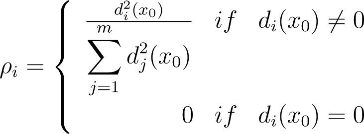
Given a bounded function, f, and x₀ ∈ D_f, we define a discrete probability distribution, P_x0, in order to present the pointwise leader entropy Considering m resolution levels, we have for i = 1,…, m,

(47)

where d_i (x₀) is the wavelet leader coefficient for x₀ and resolution level i. The probability distribution is given by P_x0 = (ρ₁,…, ρ_m). The pointwise wavelet leaders entropy for x₀ ∈ D_f is:

$$S_f(x_0)=S(P_{x0})=-{\displaystyle \sum _{i=1}^m{\rho }_i{\log }_2({\rho }_i)}$$

(48)

(if ρ_i = 0, we consider log₂ (ρ_i) = 0). We can see that if the biggest wavelet coefficients, in a neighborhood of x₀, belong to the highest resolution level (indicating more roughness), then the wavelet coefficients for x₀ are equal and S_f (x₀) is maximum (equal to log₂(m)). If, on the other hand, the wavelet coefficients for the neighborhood of x₀ are near zero, then S_f (x₀) ≈ 0.

4. Numerical Experiments

In this section, we report some numerical experiments, related to the market efficiency topics and local regularity presented in the paper, applied to the Portuguese PSI20 Index data.

This is a stock market index for the twenty most relevant assets, traded on the Euronext Lisbon, a small dimension market. These assets are selected and weighted according to their market capitalization and liquidity. The composition of the index is revised regularly. From the twenty stocks, a small number hold the majority of market capitalization. PSI20 has a non-negligible correlation with the main European stock markets.

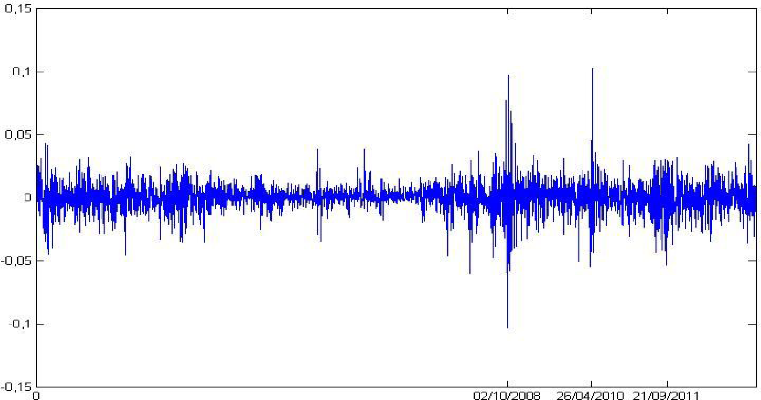
The data was collected from the Yahoo Finance publicly available database. We store settlement prices from 2000 to 2013. Let x be the vector of PSI20 settlement prices from 24 January 2000 to 24 May 2013, and N its length. Figure 1 plots the index continuously compounded returns:

$$\begin{array}{cc}r(t)=\ln (x(t+1))-\ln (x(t)),& t=1\dots N.\end{array}$$

(49)

4.1. Market Efficiency

Fractal dimension results are presented in

Table 1. The fractal dimension.

	PSI20 log-prices	Estimated Integrated variance of PSI20 log-prices
Hall–Wood	1.43	1.00
Genton	1.43	1.03
Box-count	1.38	1.04

, for the log prices series and the corresponding estimated values of the integrated variances. These are estimated through the realized variances (RV), which for log-prices are given by:

$$RV(t)={\displaystyle \sum _{i=1}^t{[log(x(i))-log(x(i-1))]}^2={\displaystyle \sum _{i=1}^t{(r(i))}^2,t=1\dots ,N}}$$

We consider different approaches, such as Hall–Wood, Genton and box-counting estimators (see [23–25,37]), applied to the PSI20 log-prices and to the estimated series of integrated variance.

The reference value for the fractal dimension is 1.5, which stands for the absence of either local persistence or local anti-persistence. If the fractal dimension is greater (resp. smaller) than 1.5, it means that there is local anti-persistence (resp. persistence), and the series path is rougher (resp. less rough) than in the reference case.

For log-prices, the values we found are slightly less than 1.5, indicating that there is no significant local persistence. As for the estimated series of integrated variance, we obtain values close to unity, which means that there is strong local persistence.

The Hurst coefficient was computed with different approaches, such as Geweke Porter-Hudak, periodogram and R/Sestimators; see [17,19,20,38]. We considered the PSI20 returns and the square of these returns; the results are shown in

Table 2. The Hurst coefficient.

Hurst	PSI20 returns	Squared PSI20 returns
GPH	0.5483 (conflo = 0.3148, confhi = 0.6852)	0.799
Periodogram	0.528	0.7456
R/S	0.5774	0.8845

.

The reference value for the Hurst coefficient is 0.5, which stands for the absence of either positive long memory or negative long memory. If the Hurst coefficient is greater (resp. smaller) than 0.5, then there is positive (resp. negative) long memory in the series.

In our data, there is long memory in the squared return series (representing volatility), but not in the returns series (as observed in general, in the empirical literature; see [39–41]).

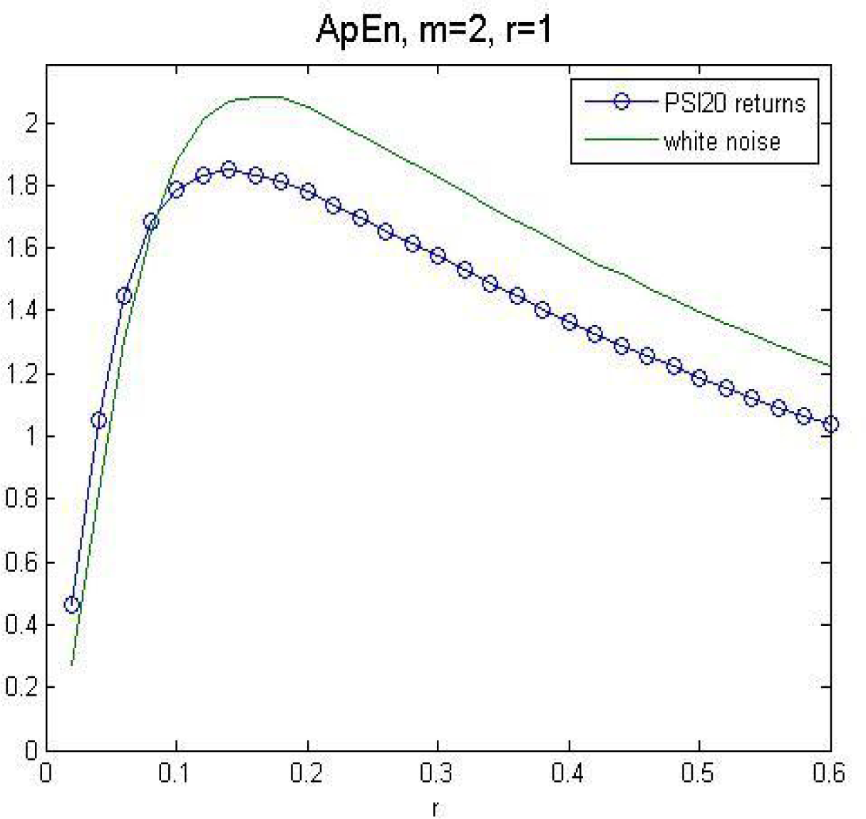
In Figure 2, we compare the approximate entropy from the returns series to the approximate entropy from a white noise process, for m = 2 and r = 1. The nearness of the curves indicates that PSI20 returns have a high degree of unpredictability.

For the q-triplet, the reference value is one (see, for instance, [6,9]).

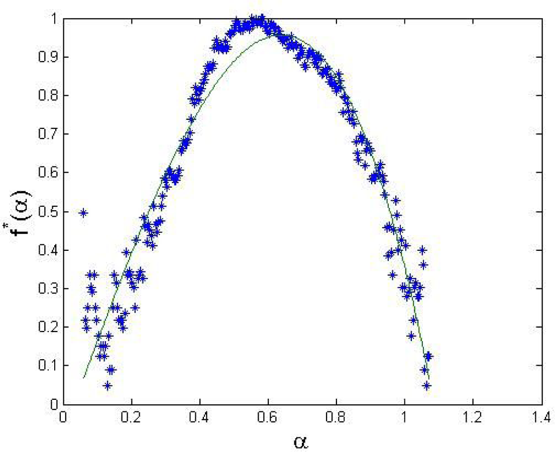
In our data, the q-triplet assumes the following results: q_rel = 1 for the PSI20 returns (the fact that there are negative correlations in the returns indicates that there is no long memory) and q_rel = 1.5 in the squared returns, indicating long memory in volatility; q_stat = 1.44 (either using a maximum likelihood method or using the scaling based method), which indicates rougher paths than in the Gaussian reference case; q_sens = 0.541 (obtained using the multifractal spectrum estimated for the PSI20 returns and a third order polynomial approximation, presented in Figure 3); we have q_sens < 1, which means that the return series is sensitive to initial conditions (as opposed to insensitivity if q_sens > 1).

4.2. Wavelet Leader Entropy

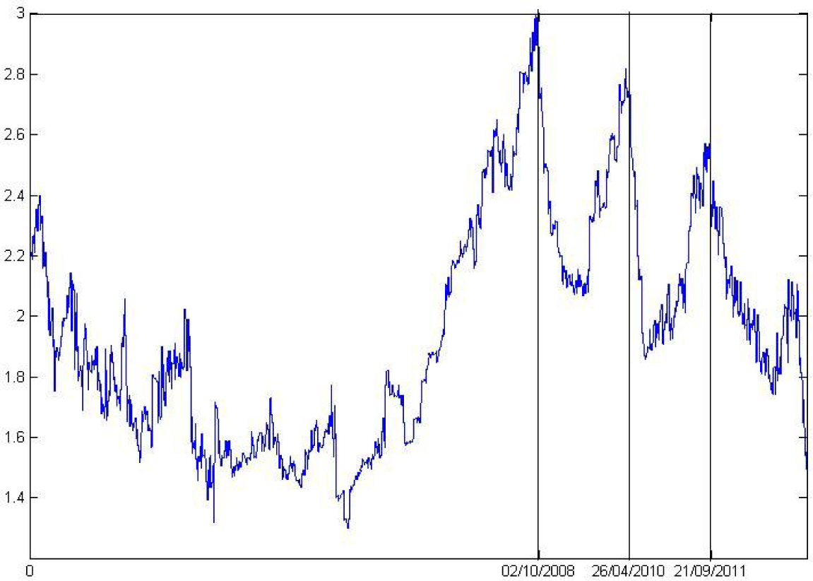
There is an inverse relation between the pointwise Hölder exponent and the pointwise wavelet leader entropy, as we pointed out before. We computed the wavelet coefficients considering an orthogonal decimated discrete wavelet transform; our mother wavelet is a Daubechies, with three vanishing moments. After computing the wavelet leader coefficients for the return series, we estimate the temporal evolution of the pointwise wavelet leader entropy (see Figure 4).

The entropy is considered to be the maximum when we have the most uncertain situation. Wavelet leader values near log₂ (8) (eight is the number of scales from the wavelet decomposition) indicate high regularity in the signal, while values near zero indicate low regularity. The temporal evolution of regularity allows one to identify a crisis; the financial crisis of 2008 and subsequent local minimums in PSI20 returns. Those dates are indicated in Figure 4. In fact, this entropy presents sharp peaks at these temporal moments (when we obtain values near log₂ 8 for the pointwise wavelet leader entropy, we expect an irregularity in the signal).

5. Concluding Remarks

In our estimations, we find that the PSI20 returns series is highly unpredictable, rougher than a normally distributed series and has no long memory (but has persistent volatility). These characteristics are typical findings in an efficient market. The analysis of local regularity, using wavelet leaders, allows one to identify the moments of a crash in the Portuguese market as those where a peak, in the degree of irregularity, is attained. Therefore, this technique may be seen as a means to identify those kinds of events.

References

- Kristoufek, L.; Vosvrda, M. Measuring capital market efficiency: Global and local correlations structure. Physica A 2013, 392, 184–193. [Google Scholar]
- Kristoufek, L.; Vosvrda, M. Commodity futures and market efficiency. Energ. Econ 2014, 42, 50–57. [Google Scholar]
- Fama, E. The Behavior of Stock-Market Prices. J. Bus 1965, 38, 34–105. [Google Scholar]
- Samuelson, P. Proof That Properly Anticipated Prices Fluctuate Randomly. Ind. Manag. Rev 1965, 6, 41–49. [Google Scholar]
- Brockwell, P.; Davis, R. Introduction to Time Series and Forecasting, 2nd ed; Springer: New York, NY, USA, 2002. [Google Scholar]
- Tsallis, C. Dynamical scenario for nonextensive statistical mechanics. Physica A 2004, 340, 1–10. [Google Scholar]
- Pavlos, G.; Karakatsanis, L.; Xenakis, M.; Sarafopoulos, D.; Pavlos, E. Tsallis statistics and magnetospheric self-organization. Physica A 2012, 391, 3069–3080. [Google Scholar]
- Ferri, G.; Reynoso-Savio, M.; Plastino, A. Tsallis’ q-triplet and the ozone layer. Physica A 2010, 389, 1829–1833. [Google Scholar]
- De Freitas, D.; Franc¸a, G.; Scheerer, T.; Vilar, C.; Silva, R. Non-extensive triplet in geological faults system. Europhys. Lett 2013, 102, 39001–39006. [Google Scholar]
- De Souza, J.; Rostirolla, S. A fast MATLAB program to estimate the multifractal spectrum of multidimensional data: Application to fractures. Comput. Geosci 2011, 37, 231–249. [Google Scholar]
- Queirós, S.; Moyano, L.; de Souza, J.; Tsallis, C. A nonextensive approach to the dynamics of financial observables. Eur. Phys. J. B 2007, 55, 161–167. [Google Scholar]
- Jaffard, S. Wavelet Techniques in Multifractal Analysis. In Fractal Geometry and Applications: A Jubilee of Benoît Mandelbrot; American Mathematical Society: Providence, RI, USA, 2004; Volume 72, pp. 91–151. [Google Scholar]
- Wendt, H.; Abry, P. Multifractality tests using bootstrapped wavelet leaders. IEEE Trans. Signal Process 2007, 55, 4811–4820. [Google Scholar]
- Rosenblatt, M.; Serrano, E.; Figliola, A. An entropy based in wavelet leaders to quantify the local regularity of a signal and its application to analize the Dow Jones index. Int. J. Wavelets Multiresolut. Inf. Process 2012, 10, 1250048. [Google Scholar]
- McLeod, A.; Hipel, K. Preservation of the rescaled adjusted range: 1. A reassessment of the Hurst phenomenon. Water Resour. Res 1978, 14, 491–508. [Google Scholar]
- Hall, P. Defining and Measuring Long-Range Dependence. In Nonlinear Dynamics and Time Series: Building a Bridge between the Natural and Statistical Sciences; Cutler, C., Kaplan, D., Eds.; American Mathematical Society: Providence, RI, USA, 1997; Volume 11, pp. 153–160. [Google Scholar]
- Lo, A. Long-Term Memory in Stock Market Prices. Econometrica 1991, 59, 1279–1313. [Google Scholar]
- Cox, D. Contribution to discussion of paper by A.J. Lawrance and N.T. Kottegoda. J. R. Stat. Soc 1977, 34, 140–145. [Google Scholar]
- Geweke, J.; Porter-Hudak, S. The estimation and application of long memory time series model. J. Time Anal 1983, 4, 221–238. [Google Scholar]
- Hurst, H. Long term storage capacity of reservoirs. Trans. Am. Soc. Civ. Eng 1951, 116, 770–779. [Google Scholar]
- Newey, K.; West, D. A Simple, Positive Semi-definite, Heteroskedasticity and Autocorrelation Consistent Covariance Matrix. Econometrica 1987, 55, 703–708. [Google Scholar]
- Robinson, P. Gaussian Semiparametric Estimation of Long Range Dependence. Ann. Stat 1995, 23, 1630–1661. [Google Scholar]
- Theiler, J. Estimating fractal dimension. J. Opt. Soc. Am. A 1990, 7, 1055–1073. [Google Scholar]
- Hall, P.; Wood, A. On the performance of box-counting estimators of fractal dimension. Biometrica 1993, 80, 246–252. [Google Scholar]
- Genton, M. Highly Robust Variogram Estimation. Math. Geol 1998, 30, 213–221. [Google Scholar]
- Pincus, S. Approximate entropy as a measure of system complexity. Proc. Natl. Acad. Sci. USA 1991, 88, 2297–2301. [Google Scholar]
- Pincus, S.; Gladstone, I.; Ehrenkranz, R. A regularity statistic for medical data analysis. J. Clin. Monitor 1991, 7, 335–345. [Google Scholar]
- Pincus, S.; Kalman, R. Irregularity, volatility, risk, and financial market time series. Proc. Natl. Acad. Sci. USA 2004, 101, 13709–13714. [Google Scholar]
- Lyra, M.; Tsallis, C. Nonextensivity and Multifractality in Low-Dimensional Dissipative Systems. Phys. Rev. Lett 2004, 80, 53–56. [Google Scholar]
- Darooneh, A.; Naeimi, G.; Mehri, A.; Sadeghi, P.; Tsallis, Entropy; Escort, Probability. the Incomplete Information Theory. Entropy 2010, 12, 2497–2503. [Google Scholar]
- Cortines, A.; Riera, R. Non-extensive behavior of a stock market index at microscopic time scales. Physica A 2007, 377, 181–192. [Google Scholar]
- Jensen, A.; la Cour-Harbo, A. Ripples in Mathematics; Springer: Berlin/Heidelberg, Germany, 2001. [Google Scholar]
- Percival, D.; Walden, A. Wavelet Methods for Time Series Analysis; Cambridge University Press: Cambridge, UK, 2000. [Google Scholar]
- Mallat, S. A Wavelet Tour of Signal Processing, the Sparse Way; Elsevier: New York, NY, USA, 2009. [Google Scholar]
- Genc¸ay, R.; Selçuk, F.; Whicther, B. An Introduction to Wavelets and Other Filtering Methods in Finance and Economics; Academic Press: Waltham, MA, USA, 2002. [Google Scholar]
- Daubechies, I. Ten Lectures on Wavelets, 1st ed; SIAM: Philadelphia, PA, USA, 1998. [Google Scholar]
- Gneiting, T.; Sevcíková, H.; Percival, D.B. Estimators of Fractal Dimension: Assessing the Roughness of Time Series and Spatial Data. Stat. Sci 2012, 27, 247–277. [Google Scholar]
- Zivot, E.; Wang, J. Modeling Financial Time Series with S-PLUS; Springer: New York, NY, USA, 2006. [Google Scholar]
- Cont, R. Empirical properties of asset returns: Stylized facts and statistical issues. Quant. Financ 2001, 1, 223–236. [Google Scholar]
- Baillie, R. Long Memory Processes and Fractional Integration in Econometrics. J. Econom 1996, 73, 5–59. [Google Scholar]
- Baillie, R.; Bollerslev, T.; Mikkelsen, H. Fractionally Integrated Generalized Autoregressive Conditional Heteroskedasticity. J. Econom 1996, 74, 3–30. [Google Scholar]