Randomized Binary Consensus with Faulty Agents

Abstract

This paper investigates self-organizing binary majority consensus disturbed by faulty nodes with random and persistent failure. We study consensus in ordered and random networks with noise, message loss and delays. Using computer simulations, we show that: (1) explicit randomization by noise, message loss and topology can increase robustness towards faulty nodes; (2) commonly-used faulty nodes with random failure inhibit consensus less than faulty nodes with persistent failure; and (3) in some cases, such randomly failing faulty nodes can even promote agreement.

1. Introduction

The use of consensus algorithms is reported in various systems, ranging from distributed database management [1], to detection [2] and mission planning [3].

Networked algorithms for distributed decision-making, operating in real-life systems, should be robust towards various disturbances. Studies on the robustness of consensus algorithms investigate the influence of noise [4,5], message loss [6], random topologies [7] and faulty node behavior [8]. Faulty nodes are often considered as one of the main impediments to consensus [8,9].

Scholars approach the problem of fault tolerance with fault-detection [10,11], increasing system-wide synchrony [12,13] and randomization. Randomization is a technique that utilizes random processes (that are often considered as negative disturbances) to increase fault tolerance [14]. Unlike fault-detection, randomization does not significantly increase the complexity of the algorithm and does not require system-wide adjustments, such as an imposed synchrony. Studies show that randomization can be beneficial for consensus, both in terms of efficiency [14,15] and fault tolerance [14,16]. Recent studies show that such beneficial randomization can sometimes be provided explicitly by noise [17,18] or errors [15].

This motivated us to investigate the impact of faulty nodes on self-organized binary majority consensus. In this article, we focus on faulty nodes with persistent and random failure and different layouts over the network. We study the influence of the faulty nodes in ring lattices and Watts–Strogatz [19] and Waxman [20] networks randomized by message loss, additive noise and topology randomization.

We show that the decrease in efficiency induced by faulty nodes can be mitigated by the randomization of different origin. We show that commonly-used faulty nodes with random failure and faulty nodes with random full failure are less adverse for consensus than faulty nodes with persistent failure. Finally, we show that in some cases, randomization by faulty nodes can even promote consensus.

The article is organized as follows. Section 2 gives a short overview of related work. Section 3 describes system modeling. Section 4 presents simulation results and analysis. Finally, Section 5 concludes the article.

2. Related Work

Self-organization is a phenomenon often observed in systems, where simple local interactions of networked agents can produce global coordination [21–23]. Networked control algorithms, inspired by such systems, can be efficient and robust [24]. Binary majority consensus exhibits self-organizing features: it is performed by simple rules in a distributed manner and can show an increase in efficiency with stochastic intrusions [15,25]. Studies on self-organized consensus can provide practical insights on the engineering of networked control systems. In this article, we focus on simple binary majority consensus algorithms to investigate whether randomization can have a positive effect not only on its efficiency, but also on its robustness.

2.1. Distributed Binary Majority Consensus

In this article, we focus on a wait-free binary majority consensus—a sub-class of the general consensus. Consensus algorithms are a class of algorithms that aim to provide a common decision for all nodes in a networked system and satisfy the following conditions [14]:

(1)

Agreement: all nodes choose the same value.

(2)

Termination: all non-faulty nodes eventually decide.

(3)

Validity: the common output value is an input value of some node.

Let us briefly specify the wait-free binary majority consensus (BMC) in this perspective. Binary majority consensus is a sub-class of consensus algorithms with specific agreement and termination conditions. Binary majority consensus algorithms provide that a network agrees on state that is selected out of limited set of binary inputs, generally defined as {0, 1} or {−1, 1}. The agreed state should correspond to the initial majority of all states in the network. A wait-free requirement specifies a termination condition: such algorithms are terminated after a predefined time, T, whether agreement was reached or not. Wait-free binary majority consensus can be beneficial in real-life networked systems, where the termination time is important. Time limitation, however, can lead to lower efficiency and higher sensitivity to disturbances [15,26,27].

The strict termination conditions of BMC make it difficult to guarantee the agreement. Due to this efficiency of the binary majority, consensus is registered as convergence rate, R—a fraction of initial network configurations that result in successful agreement. BMC has been actively studied since Gacs et al. [26] introduced the Gacks–Kurdyumov–Levin (GKL) consensus that provides R ≃ 82%. This convergence rate was registered in a synchronized ring lattice of N = 149 nodes, where each node is connected to its 2K = 6 neighbors. Since then, most scholars adopted this network as a reference case for comparing the convergence rate of BMC algorithms. In the last several decades, several solutions slowly advanced the R up to 86% [28]. Land and Belew [29] show that a deterministic algorithm cannot solve the consensus with 100% efficiency in a reference setup. This motivated research on randomized solutions that advanced the convergence rate up to 90% [15,30]. However, proposed solutions only work in a limited set of synchronous networks and were not tested for robustness towards faulty node behavior.

2.2. Fault Tolerance of Consensus

Studies on the robustness and the fault tolerance of general consensus algorithms consider faulty nodes as one of the main impediments to consensus. Faulty nodes are generally represented as Byzantine faulty nodes—nodes that can have any arbitrary failure, except full failure. Early study by Pease et al. [31] shows that in a synchronized networked system of N nodes, M of them being faulty, consensus is possible if $M<\frac{N-1}{3}$. Later, Fischer et al. [8] strengthened this condition for asynchronous systems, showing that consensus may become impossible with already M = 1.

Due to strict termination conditions, BMC can be sensitive to the faulty node behavior. Specific cases of BMC with faulty nodes have been previously studied in [32] and [17]. Thus, [32] reports that simple majority (SM) consensus is more strongly inhibited by faulty nodes with persistent failure than by faulty nodes with random failure in some networks. Another affect is reported in [17], where it is shown that Gacs–Kurdyumov–Levin (GKL) and SM consensus inhibited by a low number of faulty nodes with persistent failure can restore the convergence rate with randomization.

This article complements and extends these works for a wider range of network models, types of disturbances and faulty nodes. We study BMC with faulty nodes in ring lattices, Watts–Strogatz and Waxman networks with various stochastic disturbances. We consider persistently and randomly failing faulty nodes in networks with a random and clustered faulty node layout. We show that randomization by topology, noise and message loss can mitigate the decrease in efficiency induced by faulty nodes of different types. We also show that in some cases, faulty nodes with random failure can even promote consensus. Finally, we explain and illustrate the mechanisms behind these effects with convergence analysis.

3. Experimental Setup

3.1. Network Model

We investigate BMC in ring lattices and randomized Watts–Strogatz (WS) [19] and Waxman [20] networks. A Watts–Strogatz graph can produce networks, ranging from ordered grids to small-world and fully random networks. Due to this, WS networks are widely used to model systems interactions, spanning from technical systems [15] to natural [33] and social networks [34]. Graphs proposed by Waxman [20], on the other hand, are widely used to model human-designed random networks, like the Internet [35]. These types of systems compliment each other and allow us to compare the efficiency of the algorithms with the preceding solutions and to cover major network models for areas, where consensus algorithms found their use.

3.1.1. Ring Lattices

To model ring lattices, we follow a reference network design introduced in [26]. Such a network is initially created as a one-dimensional cellular automaton of N nodes, connected to their 2K closest neighbors. This automaton is then closed in a ring to avoid boundary effects. Such a setup is often used to register the convergence rate of BMC [30,36,37]. Neighbors of each node, i ∈ {0,…, N}, are split into three sets: the set of all neighbors N_i, ‖N_i‖ = 2K, N_i = {i − K,…, i − 1, i + 1,…, i + K}; the set of left-side neighbors N_l, ‖N_l‖ = K, N_l = {i – K,…, i − 1,}; and the set of right-side neighbors N_r, ‖N_r‖ = K, N_r = {i + 1,…, i + K}. These sets are further used by consensus algorithms to access neighbors’ state information. For comparison purposes, for all algorithms, we use K = 3, initially defined for GKL in [26]. Here and further, we study undirected graphs and refer to the “link” as the connection between nodes i and j. For ring lattices and WS networks, a “link length” between nodes i and j is defined as the difference between their respective indices. For Waxman networks, link length is an actual Euclidean distance, randomly chosen in the beginning of simulation. Random and complex networks, such as WS and Waxman graphs, are often characterized with the path lengths that are composed of multi-hop connections. The simple consensus algorithms studied in this paper only account for the closest, one-hop neighborhood of each node. Due to this, we characterize the networks with “link length” and “node degree” rather than a “path length”.

3.1.2. Watts–Strogatz Networks

A Watts–Strogatz graph can produce networking models ranging from ordered grids to fully random networks. It is initially modeled as a one-dimensional ring of N nodes, where each node is connected with the next K nodes. Further, with rewiring probability P ∈ [0, 1], each link of the node, i, is substituted with a link to a random node j ∉ {i − K,…, i + K}, i.e., at P = 0, a network is a 2K-connected ordered grid of N nodes. At P = 0.5, approximately half of the links is substituted with random ones, and the network can be represented as a small-world graph. Finally, at P = 1, all links are random, and the network is a fully random graph.

3.1.3. Waxman Networks

A Waxman graph is built as follows. First, for each pair of nodes, i, j ∈ {1, 2,…, N}, i ≠ j, the distance, d, is randomly uniformly chosen from the interval (0, 1]. Next, the nodes are linked with probability:

$$\alpha \exp \left(-\frac{d}{\beta }\right),$$

(1)

with parameters α, β ∈ (0, 1]. Parameters α and β influence the system as follows. An increasing α yields an increasing link probability, thus increasing the average node degree. An increasing β has an influence similar to that of P in WS networks: it increases the number of long random links compared to short links, thus increasing the average link length in the network. We model sparsely connected Waxman graphs with fixed α = 0.05 and β ∈ [0.01, 0.4]. Within the given parameter range of β, we limit the average node degree and average link length to match the WS model.

3.2. Consensus Algorithms

At the first time step t = 0, every node, i ∈ {0,…, N}, is randomly assigned with a binary state, σ_i ∈ {−1, 1}. The combination of all N initial states, σ_i, is called the initial configuration. The sum of all states in initial configuration ${\displaystyle {\sum }_{i=0}^{i=N}{\sigma }_i}[0]$ is called initial density and denoted as ρ[0].

At every time step 0 ≤ t ≤ T, each node updates its state following a given consensus algorithm, based on its own state and the state information received from neighboring nodes. Within T time steps, all nodes are expected to agree on a single state, corresponding to the initial majority (density); i.e., a network is converged if there exist time t_c ≤ T, so that ${\displaystyle {\sum }_{i=0}^{i=N}{\sigma }_i}[t_c]=N$ for ρ[0] > 0 or ${\displaystyle {\sum }_{i=0}^{i=N}{\sigma }_i}[t_c]=-N$ for ρ[0] < 0. We use T = 2N, as initially defined in [26].

In this article, we focus on the randomized Gacs–Kurdyumov–Levin and simple majority consensus algorithms, which we will now briefly describe.

3.3. Simple Majority Consensus

With simple majority consensus, every node updates its state on the basis of its own state and the state information received from its neighbors.

$${\sigma }_i[t+1]=G\left({\sigma }_{i,i}[t]+{\displaystyle \sum _{j\in N_i}{\sigma }_{i,j}}[t]\right).$$

(2)

Here, σ_i,j[t] denotes the state of the node, j, at the time, t, received by the node, i. The update function, G(x), is defined as in [15,25]:

$$G(x)+\{\begin{array}{cc}-1& \text{for}x<0,\\ +1& \text{for}x>0.\end{array}$$

(3)

SM consensus is arguably the simplest algorithm for binary majority sorting and has a balanced design: In ring lattices, each node, i, receives an equal number of messages from both sides of the lattice. Due to this, SM indicates a low convergence rate in ordered and noiseless systems, but in strongly randomized setups, it can show a high convergence rate [15,17,32] and outperform GKL.

One can see that G(x) is not defined for x = 0, which is a valid assumption for undisturbed networks where an odd number of received state messages ensures that their sum is always either negative or positive. However, in noisy networks or in networks with message loss, a sum of received state messages can sometimes be equal to 0. For this case, we adjust G(x) in the following manner: If a decision cannot be made (i.e., when the sum of received state messages is equal to 0), the state of the node remains unchanged: σ_i[t + 1] = σ_i[t].

3.4. Gacs–Kurdyumov–Levin Consensus

GKL consensus is known to be among the best algorithms for binary majority problem [36]. It is simple, efficient and is often used as a benchmark for new algorithms [30,37,38]. Nodes driven by GKL update their states as follows. Depending on its own current state, each node chooses which side to receive messages from: If σ_i,i[t] < 0, node i receives state information from the first and the third neighbor to the left; if σ_i,i[t] > 0, it receives information from the first and the third neighbor to the right.

$${\sigma }_i[t+1]=\{\begin{array}{cc}G\left({\sigma }_{i,i}[t]+{\sigma }_{i,l_3}[t]+{\sigma }_{i,l_3}[t]\right)& \text{for}{\sigma }_{i,i}[t]<0,\\ G\left({\sigma }_{i,i}[t]+{\sigma }_{i,r_1}[t]+{\sigma }_{i,r_3}[t]\right)& \text{for}{\sigma }_{i,i}[t]>0.\end{array}$$

(4)

Here, l₁, l₃ and r₁, r₃ are the first and the third neighbors of the node, i, to the left and to the right, respectively. One can see that, essentially, GKL is a modification of SM consensus with a built-in state-direction bias. This bias provides for the high efficiency of GKL in ring lattices, but it can lead to low efficiency if the network structure or the update sequence are disturbed [15,17].

3.5. Update Mode

System-wide synchrony can be crucial for consensus process [12,13]. We simulate systems with synchronous and asynchronous update functions. In the synchronous mode, all nodes update their states simultaneously. In the asynchronous mode, nodes are updated sequentially, one after the other, according to their indices, i.e., 0 → N. To update its state, a node uses the latest available states of its neighbors.

3.6. Initial Configurations

For our simulations, we use test sets combined of 10⁴ initial configurations. Each initial configuration is composed of N initial states, σ_i, obtained as a result of a coin-flip operation, returning 1 or −1 with equal probability, as in [15,26].

3.7. Faulty Nodes Modeling

We study faulty nodes with two failure models: faulty nodes with random failure, modeled after the Byzantine failure model, and faulty nodes with persistent failure.

We implement faulty nodes as follows. At a starting time t = 0, M faulty nodes are added to N non-faulty nodes to avoid the bias of the initial configuration. Network topology is then created for all N + M nodes. After adding M faulty nodes to the system, they are labeled as faulty and counter consensus, according to their failure model.

3.7.1. Faulty Node Layout

We use two schemes of the faulty node layout: clustered and distributed. With the clustered layout, all faulty nodes are located next to each other. The location of the cluster is randomly chosen at each simulation run. With the distributed layout, all faulty nodes are randomly placed over the network independent from each other.

3.7.2. Faulty Nodes with Random Failure

We implement faulty nodes with random failure after commonly-used Byzantine random failure with a reduced state space. Such nodes randomly change their broadcast state, independently of the state information received from their neighbors. We investigate two types of faulty nodes:

• two-state faulty nodes, randomly switching between states σ_M ∈ {−1, 1}; and

• three-state faulty nodes, switching between σ_M ∈ {−1, 0, 1}.

The first case presents a faulty node that broadcasts correct and erroneous state information with equal probabilities. The second case additionally implements a state of sending no information, i.e., a full failure.

3.7.3. Faulty Nodes with Persistent Failure

Faulty nodes with persistent failure are modeled as follows. After M faulty nodes are added, they are assigned with a faulty value, σ_M, opposite to the initial majority: if ${\displaystyle {\sum }_{i=0}^{i=N}{\sigma }_i}[0]<0,{\sigma }_M=1$; and if ${\displaystyle {\sum }_{i=0}^{i=N}{\sigma }_i}[0]>0,{\sigma }_M=-1$. During the consensus process, such faulty nodes broadcast their state, but do not update it. Unlike faulty nodes with random failure, faulty nodes with persistent failure provide enduring inhibition for consensus.

3.8. Additive Noise

To introduce the noise, we modify the system as follows. Recall that in the original system, node i receives state information from node j via state information message σ_i,j[t]. We implement noise added to the received state information by the following transformation:

$${\sigma }_{i,j}\left[t\right]\to {\sigma }_{i,j}\left[t\right]+{\varphi }_{i,j}.$$

(5)

Here, a random value, ϕ_i,j, is a sample of added noise. We implement two types of noise: additive white Gaussian noise (AWGN), where ${\varphi }_{i,j}\sim \mathcal{N}\left(0,{(\frac{A}{3})}^2\right)$; and additive white uniform noise (AWUN), where ${\varphi }_{i,j}\sim \mathcal{U}(-A,A)$, with the magnitude, A ∈ [0, 4]. Previous studies mostly consider AWGN as the most common noise type in real networks [5,6], and AWUN is generally used to model the response of filters and amplifiers [39]. The range for the noise amplitude, A, is chosen empirically to account for the level of disturbances that not only promote, but also hinder consensus.

3.9. Message Loss

A message loss can inhibit the BMC, since a node decision is based on an odd number of state information messages received from other nodes. If a message is lost, a node can come to a state when the sum of received state messages is equal to zero, and the state of the node stays unchanged. In our model, a state information is lost with the probability, ε_i,j ∈ [0, 1), i.e., if a message from node j to node i is lost, the received state message σ_i,j[t] = 0:

$${\sigma }_{i,j}[t]\to \{\begin{array}{l}{\sigma }_{i,j}[t],\text{with probability}(1-\epsilon )\\ 0,\text{with probability}\epsilon \end{array}.$$

(6)

In our simulations, the state information of node i is also affected by the noise and message loss, i.e., σ_i ≠ σ_i,i. This scenario corresponds to the problem of distributed detection, where nodes with unreliable sensory inputs are expected to agree whether a detected event took place. The other possible scenario assumes the influence of noise and message loss only in node-to-node communication, i.e., σ_i = σ_i,i. We omit results for this scenario, as our simulations only indicate a slight decrease of randomizing influence (both positive and negative), while the character of the influence remains the same. We investigate the impact of faulty nodes on SM and GKL in WS and Waxman networks randomized by noise, message loss and topology. In the following sections, we consequently compare the impact of faulty nodes with persistent and random failure in randomized networks with different faulty node layouts. Next, we investigate the effect of strong consensus promotion by faulty nodes with random failure, observed in [32].

4. Performance Analysis

As we mention above, the distributed binary majority consensus problem is generally solved in a wait-free manner. Additional restrictions in system connectivity and synchrony make it difficult to guarantee the convergence.

Due to this efficiency of wait-free binary majority, consensus is generally measured as convergence rate R—a fraction of initial system configurations that results in a successful agreement. For each set of parameters, we generate three random networks, which are then simulated over 30 sets of initial configurations. The resulting 90 values of R are then averaged and plotted with 95% confidence intervals.

4.1. Faulty Nodes with Random and Persistent Failure

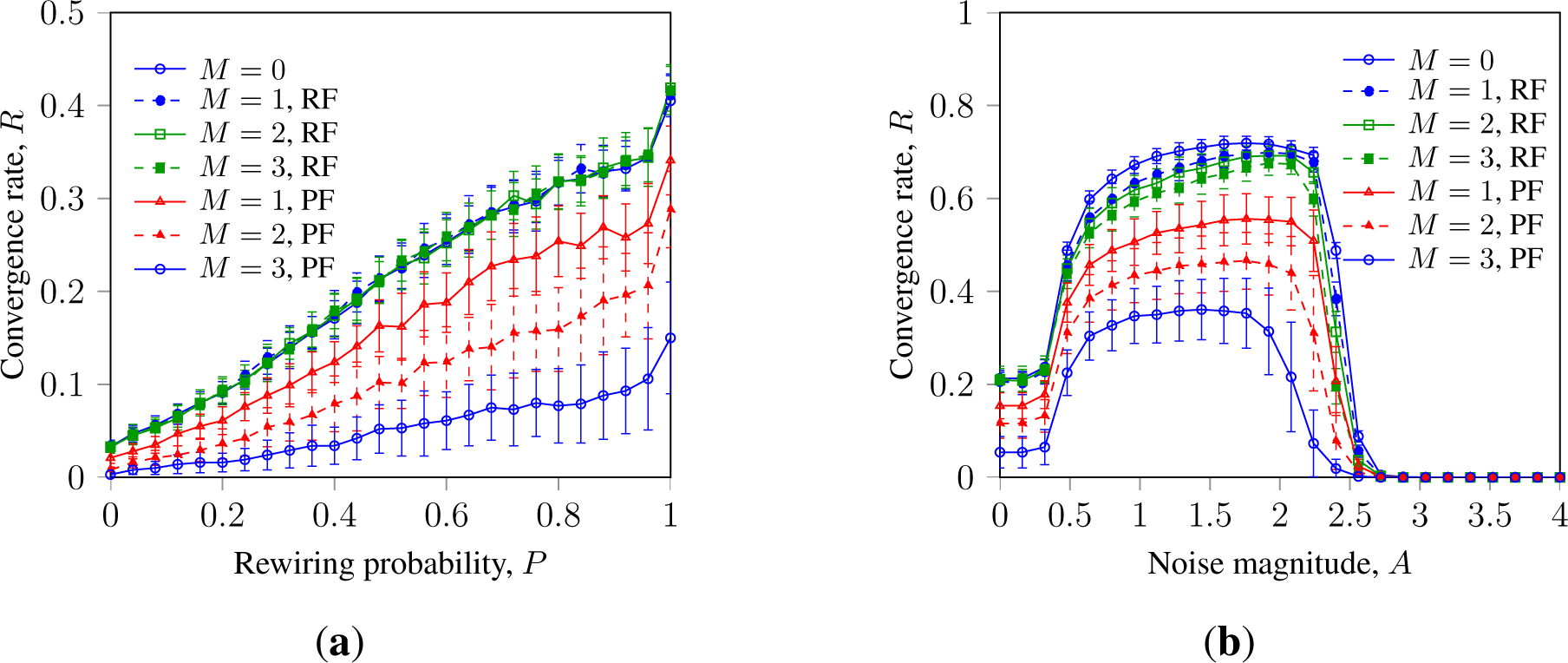
Let us analyze SM and GKL with faulty nodes and randomization by topology, noise and message loss. Figures 1a and 1b show that randomization by topology and noise can promote the robustness of SM consensus towards faulty node behavior in asynchronous and synchronized networks, respectively. It also shows that noise and topology randomization promote consensus in systems without faulty nodes (M = 0). This extends results earlier obtained in [15], where it was shown that topology randomization and a low level of errors can promote asynchronous SM.

Figure 1 also shows that faulty nodes with persistent failure inhibit consensus stronger than faulty nodes with random failure.

This can be explained as follows. Topology randomization in WS networks connects a faulty node with random neighbors, enabling the latter to overcome the reduced negative impact. Additive noise washes out the negative impact of the faulty node and promotes consensus in a similar manner. The cluster-breaking impact of randomization also contributes to the convergence rate in the systems without faulty nodes. This effect was earlier observed in [15,18,25] and can be explained as follows. Binary majority consensus is designed to provide a common decision for all nodes in the system, so the stable clusters of nodes sharing a different state inhibit the convergence. Some algorithms, like GKL, explicitly introduce the direction bias to wash out such clusters; for other algorithms, the cluster-breaking effect can be provided by stochastic disturbances.

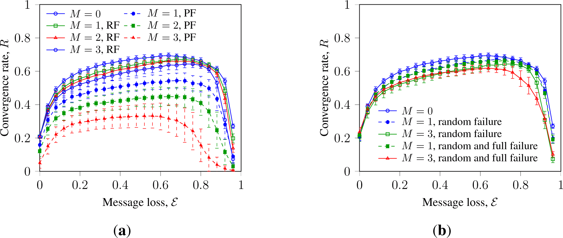
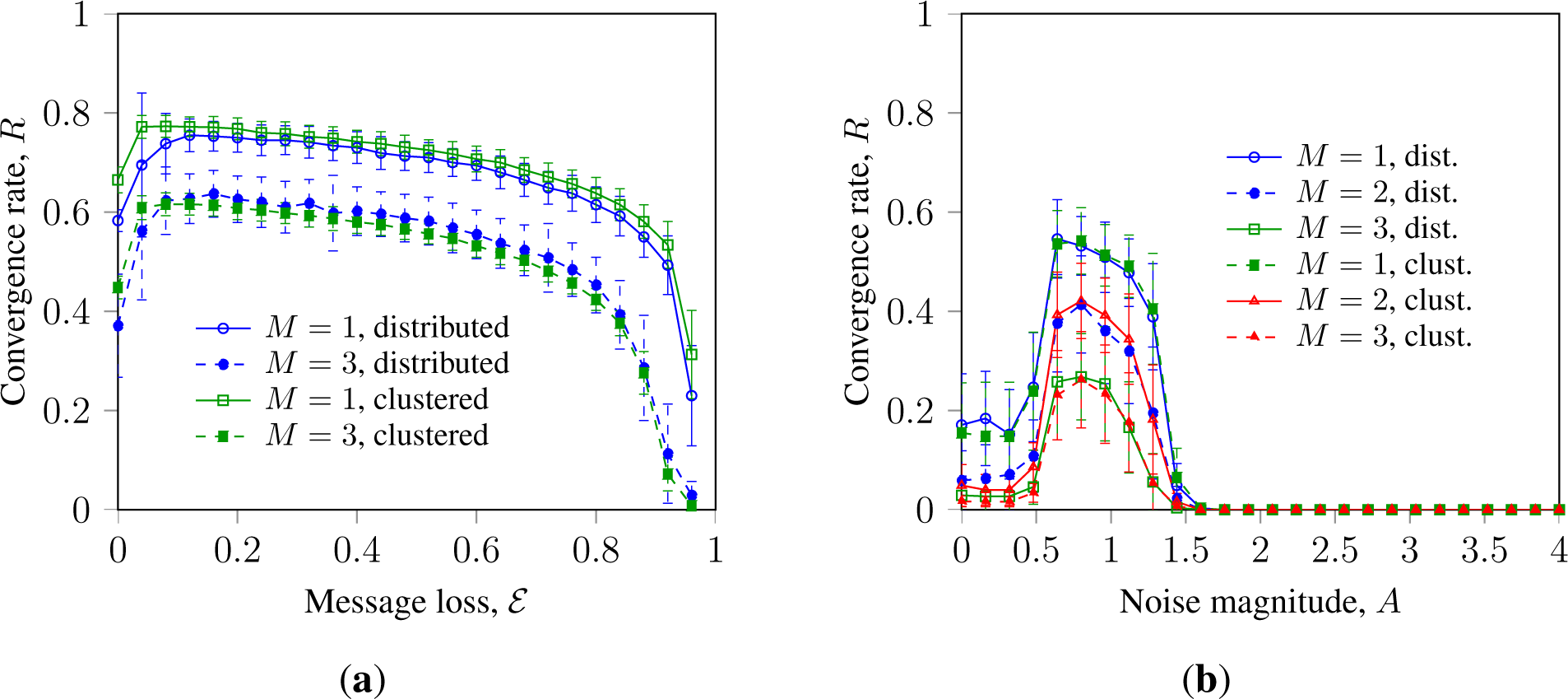
Randomization by message loss can promote consensus with faulty nodes, as shown in Figure 2. Thus, Figure 2a shows that in random WS networks, message loss can increase R of SM and GKL with faulty nodes of both types. Figure 2b shows the convergence rate of SM in random WS networks, indicating that faulty nodes with random full failure have an impact similar to that of faulty nodes with random failure.

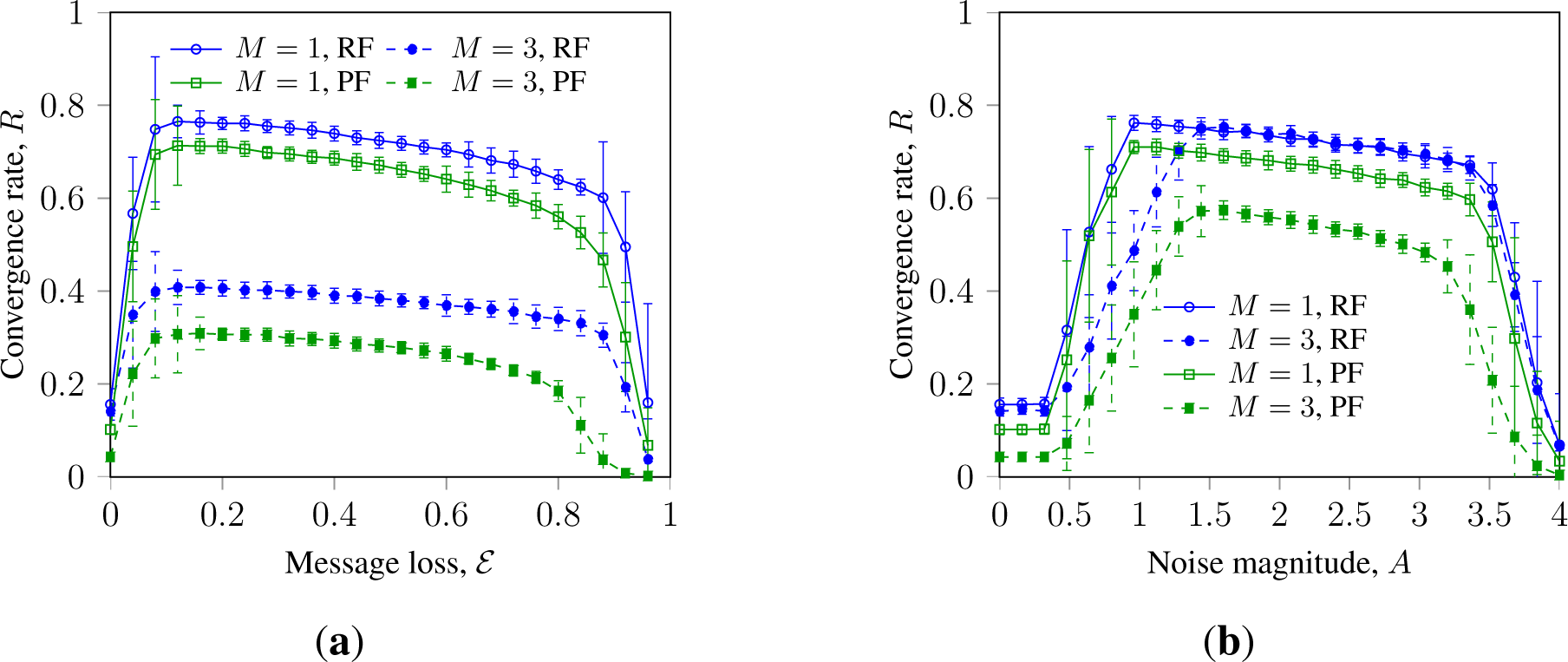
Figure 3 presents the convergence rate of SM in Waxman networks with randomization by noise and message loss. It indicates that in Waxman networks, faulty nodes with persistent failure inhibit consensus stronger than faulty nodes with random failure; an effect we earlier observed for WS networks. These observations extend the results reported in [17,32] for a wider range of network topologies and a larger scope of randomizing disturbances and faulty node types.

This can be explained by the nature of persistently failing faulty nodes: such nodes always send state information that counters the consensus process. Faulty nodes with random failures can also send correct information and, thus, contribute to the agreement.

Observed small difference in the impact between faulty nodes with random failure and faulty nodes with random full failure can be explained as follows. BMC can be promoted by stochastic message loss due to its “de-clustering” effect. Faulty nodes with stochastic full failure produce a localized impact similar to that of message loss and, thus, can promote consensus. For the same reason, such faulty nodes decrease robustness towards high levels of message loss, which can be seen in Figure 3b. This can infer the following generalization: although faulty nodes with full failure are often considered as a strong adversary for consensus, their impact on BMC indicates little difference. Moreover, both types of randomly failing faulty nodes are less adverse than persistently failing faulty nodes. Another important observation is that a number of persistent faulty nodes can be more adverse than an equal or even a bigger number of randomly failing faulty nodes. In other words, BMC systems can be more strongly inhibited with, e.g., M persistent faulty nodes with an equal number of both faulty states, σ_M ∈ {−1, 1}, than with 2M randomly failing faulty nodes.

4.2. Influence of Faulty Node Layout

In the previous section, we observed that topology randomization can mitigate the negative impact of faulty nodes. This motivated us to determine whether a static random placement of the faulty nodes can produce a similar effect in various networks, as was observed for ring lattices in [32].

We simulate networks with two types of faulty node layouts on the network where: (1) all faulty nodes are located in a single cluster; and (2) faulty nodes are randomly placed over the network.

Figures 4 and 5 present R of asynchronous GKL and SM in WS and Waxman networks with persistently failing faulty nodes with random and clustered layouts.

4.2.1. Topology Randomization

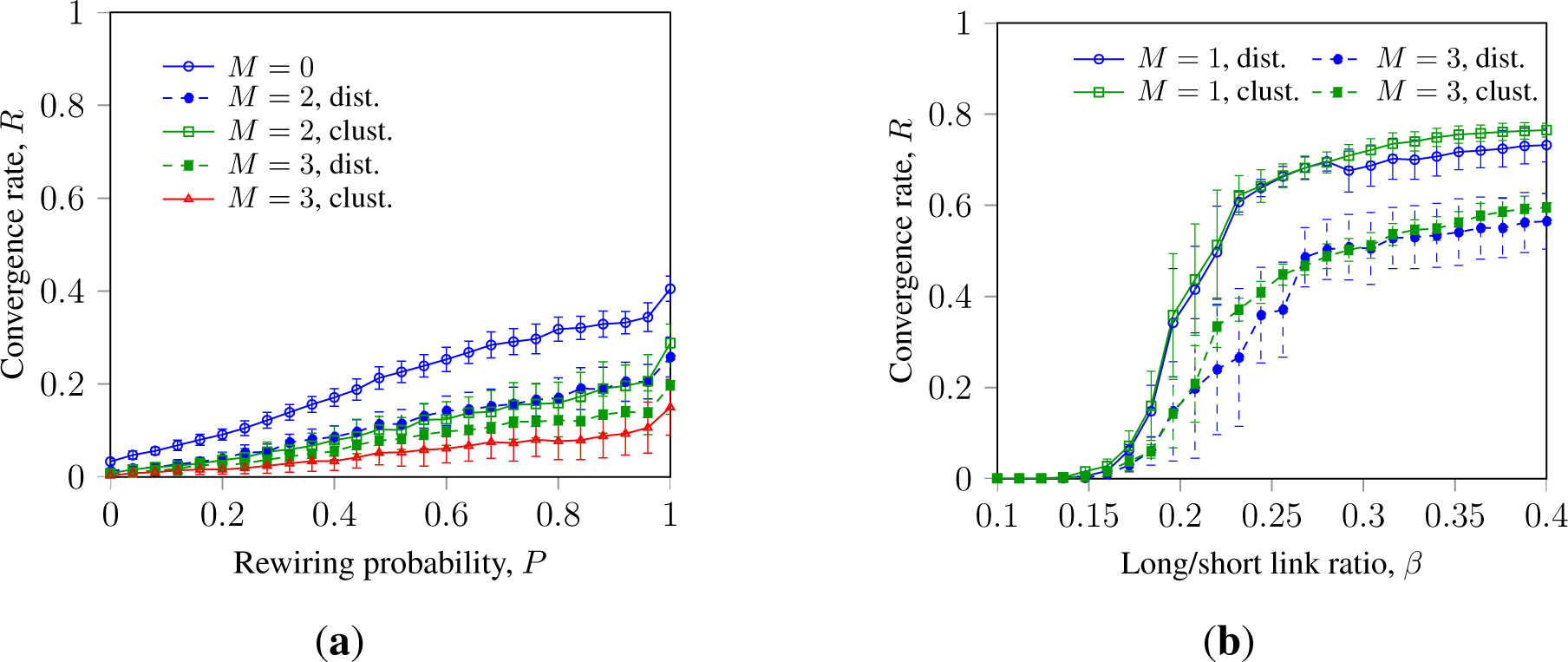
Figure 4 shows the dynamics of the SM consensus with clustered and randomly placed faulty nodes in Watts–Strogatz and Waxman networks with topology randomization (increasing P and β).

Thus, Figure 4a indicates an effect, similar to that observed earlier in [32]: in WS networks, ranging from a ring lattice (P = 0) to a random network (P = 1), faulty nodes with a clustered layout inhibit asynchronous SM slightly more strongly than faulty nodes randomly placed over the network. However, the difference in impact between clustered and randomly placed faulty nodes is low and is not observed in other setups, e.g., with synchronous SM or GKL or in Waxman networks. The difference in impact is observed with M ≥ 3 and can be explained by the sensitivity of asynchronous SM to external disturbances.

Further, Figure 4b does not indicate a notable difference in impact between clustered and randomly placed faulty nodes in the Waxman network. However, it indicates that increasing topology randomization promotes SM with faulty nodes.

4.2.2. Randomization by Noise and Message Loss in Random Networks

Figures 4b and 5 show that in random networks, the impact of clustered faulty nodes is similar to that of randomly placed ones. This can be explained by the topology randomization, which dithers the impact of the clustered faulty nodes into a wider set of nodes. This leads to the “de-clustering” of the faulty nodes and mitigates the difference in impact with randomly placed faulty nodes. This effect is observed with different types of randomization in both WS and Waxman networks, as can be seen from Figure 5. This can infer that observed difference in the impact of clustered and randomly placed faulty nodes is a feature of the asynchronous SM evident in noiseless ring lattices and WS networks.

4.3. Consensus Promotion with Randomly Failing Faulty Nodes

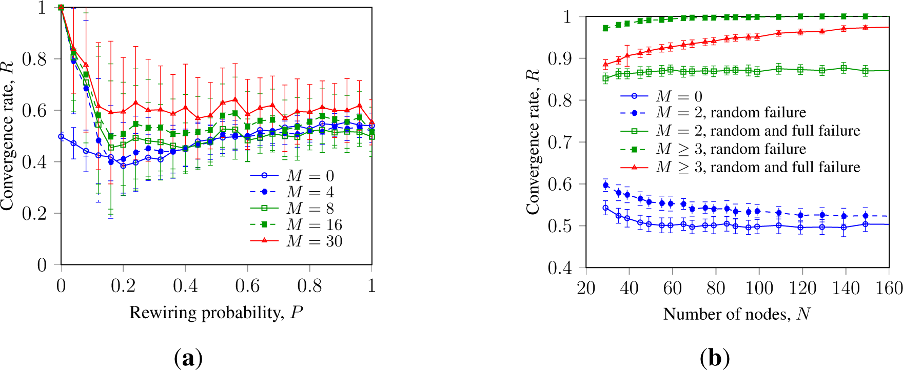
Figure 6 shows R of asynchronous GKL with clustered randomly failing faulty nodes in WS networks and ring lattices of different size. Figure 6a resembles results similar to that shown in [32], showing that M ≥ K faulty nodes located in a single cluster can significantly increase R in ring lattices (P = 0). Figure 6b shows that this effect remains with system growth. It also indicates similar consensus promotion with randomly failing faulty nodes with full failure.

The impact of randomly failing faulty nodes is more strongly expressed than the impact of randomly failing faulty nodes with full failure, though both types indicate similar dependencies. This can hint to the fact that randomization within the consensus state space can be more efficient [15,17,25].

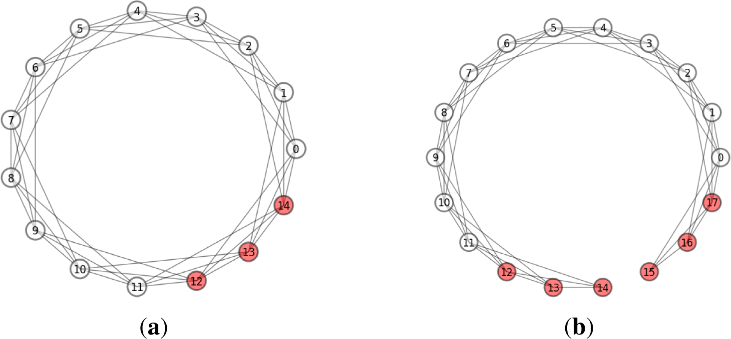
The positive impact of faulty nodes on GKL consensus can be explained by the explicit randomization they impose on the information exchange. It was previously shown that randomization by binary errors can promote consensus [15]. Positive randomization by faulty nodes reaches a maximum with M ≥ K faulty nodes located in a single cluster (see Figure 7a). Such a setup can be presented as an open one-dimensional lattice with M faulty nodes at both ends (see Figure 7b). This setup has two important features: it logically “disconnects” the network and, thus, produces boundary effects that have not been considered previously. These latter features and consensus promotion to ≃ 100% efficiency motivated us to investigate this case in more detail.

4.3.1. Convergence Dynamics

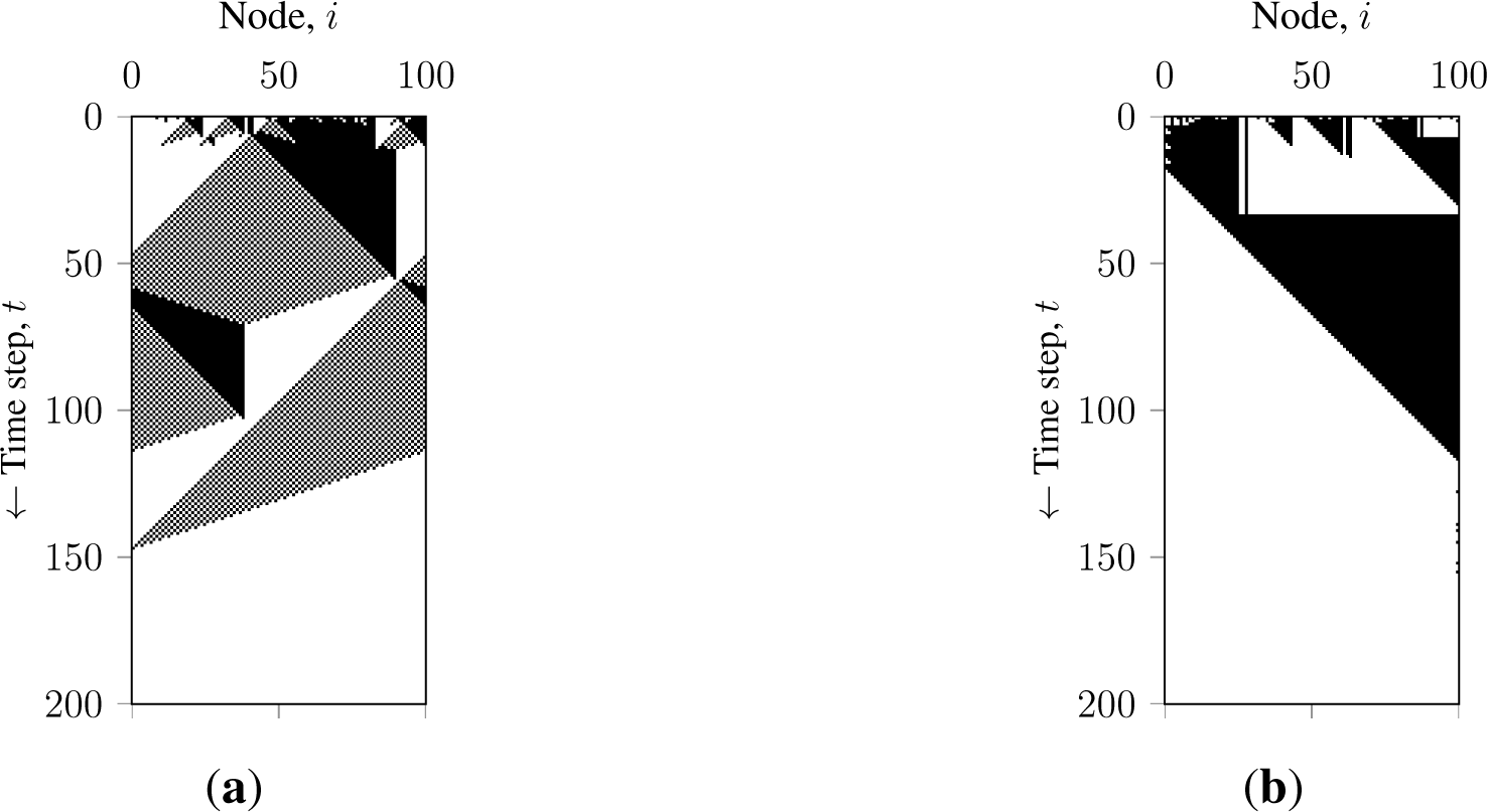
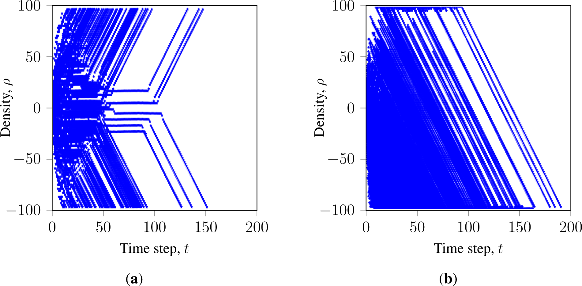
Let us study how faulty nodes promote consensus in terms of a system evolution. Figures 8 and 9 show the state and density evolution of GKL with faulty nodes over time, respectively. Figure 8a shows an agreement process of a synchronous GKL with no faulty nodes. It illustrates that in a connected ring, clusters can migrate over the network. Figure 8b shows an example of the agreement process of a synchronous GKL with M ≥ K faulty nodes. It shows that a cluster in a logically disconnected ring (see Figure 7) does not migrate and is destroyed faster. Figure 9 shows the evolutions of a GKL in a ring lattice over 500 initial configurations. Figure 9a shows the density evolution of the successfully converged networks with synchronous GKL. It illustrates that systems (each line represents a network evolving over the unique initial configuration) steadily evolve to correct majorities and terminate. Figure 9b shows the density evolution of the asynchronous GKL with M ≥ K randomly failing faulty nodes, indicating that the state direction bias of the GKL combined with asynchronous updates can steer the system to the expected state. However, it also shows that, due to stochastic intrusions, systems often evolve closely to the opposite majority and then get steered to the correct one. This happens due to the steering effect of the asynchronous sequential update and the contribution of the faulty nodes random state messages.

The latter observations can be explained as follows. Even though asynchronous GKL with additional randomization by faulty nodes can reach R ≃ 100%, it cannot be considered as a solution to the binary majority consensus problem: the system exhibits a significant measure of random dynamics and cannot guarantee a stable correct convergence in the given consensus time, T.

5. Conclusions

In this article, we study the impact of faulty nodes on randomized binary majority consensus. We simulate two standard algorithms, GKL and SM, in ordered and topologically randomized networks with noise and stochastic message loss. We study faulty nodes with persistent failure in comparison with commonly used faulty nodes with random failure, including nodes with random full failure. We simulate faulty nodes with a clustered and random layout, focusing on asynchronous networks. The main contributions of this article can be summarized as follows:

• A number of faulty nodes with persistent failure are more adverse for binary majority consensus than even a larger number of commonly-used faulty nodes with random failure or faulty nodes with random full failure;

• Simple binary majority consensus algorithms, such as simple majority, do not degrade with randomization, but respond with an increase in the convergence rate;

• Randomization by noise, message loss and topology can promote such consensus algorithms and mitigate the impact of a low number of faulty nodes.

• These new results can be explained by the “de-clustering” influence, provided by explicit stochastic intrusions, such as noise and message loss. Such consensus-promoting “de-clustering” influence, in some cases, can be provided by faulty nodes with random failure. Such nodes can promote BMC in asynchronous networks providing unstable, but efficient convergence.

This can be generalized as follows: due to restrictions in connectivity, synchrony and time, BMC exhibits diverse dynamics. This dynamics can be further exaggerated by disturbances. In particular, randomizing disturbances not only increase the efficiency of BMC, but also promote its robustness towards faulty node behavior. Consequently, stochastically failing faulty nodes present a weak adversary for such consensus and, in some cases, can even promote it. These observations can infer that the aforementioned restrictions and disturbances are not only essential requirements for the modeling of distributed consensus systems [15], but intrinsic features that help yield self-organizing behavior from simple networked interactions [24].

This work extends and complements previous investigations on binary majority consensus with stochastic elements [15,17,18,25,30,32] in terms of the robustness towards faulty node behavior.

References

- Bernstein, P.A.; Goodman, N. An algorithm for concurrency control and recovery in replicated distributed databases. ACM Trans. Database Syst 1984, 9, 596–615. [Google Scholar]
- Olfati-Saber, R.; Shamma, J.S. Consensus filters for sensor networks and distributed sensor fusion, In Proceedings of IEEE Conference on Decision and Control and European Control Conference, Seville, Spain, 12–15 December, 2005; pp. 6698–6703.
- Alighanbari, M.; How, J.P. An unbiased Kalman consensus algorithm, In Proceedings of American Control Conference, Minneapolis, MN, USA, 14–16 June 2006; pp. 3519–3524.
- Aspnes, J. Fast deterministic consensus in a noisy environment, In Proceedings of the ACM Symposium on Principles of Distributed Computing, Portland, OR, USA, 16–19 July 2000; pp. 299–308.
- Carli, R.; Fagnani, F.; Frasca, P.; Taylor, T.; Zampieri, R. Average consensus on networks with transmission noise or quantization, In Proceedings of European Control Conference, Kos, Greece, 2–5 July 2007; pp. 4189–4194.
- Kar, S.; Moura, J.M.F. Distributed average consensus in sensor networks with random link failures and communication channel noise, In Proceedings of Asilomar Conference on Signals, Systems and Computers, Pacific Grove, CA, USA, 04–07 November 2007; pp. 676–680.
- Kingston, D.B.; Beard, R.W. Discrete-time average consensus under switching network topologies, In Proceedings of American Control Conference, Minneapolis, Minnesota, MN, USA, 14–16 June 2006; pp. 3551–3556.
- Fischer, M.J.; Lynch, N.A.; Paterson, M.S. Impossibility of distributed consensus with one faulty process. J. ACM 1985, 32, 374–382. [Google Scholar]
- Fischer, M.J.; Lynch, N.A.; Merritt, M.S. Easy impossibility proofs for distributed consensus problems, In Proceedings of the ACM Symposium on Principles of Distributed Computing, Minaki, ON, Canada, USA; 1985; pp. 59–70.
- Chandra, T.D.; Toueg, S. Unreliable failure detectors for reliable distributed systems. J. ACM 1996, 43, 225–267. [Google Scholar]
- Chandra, T.D.; Hadzilacos, V.; Toueg, S. The weakest failure detector for solving consensus. J. ACM 1996, 43, 685–722. [Google Scholar]
- Dolev, D.; Dwork, C.; Stockmeyer, L. On the minimal synchronism needed for distributed consensus. J. ACM 1987, 34, 77–97. [Google Scholar]
- Dwork, C.; Lynch, N.; Stockmeyer, L. Consensus in the presence of partial synchrony. J. ACM 1988, 35, 288–323. [Google Scholar]
- Aspnes, J. Randomized protocols for asynchronous consensus. Distr. Comput 2003, 16, 165–175. [Google Scholar]
- Moreira, A.A.; Mathur, A.; Diermeier, D.; Amaral, L.A.N. Efficient system-wide coordination in noisy environments. Proc. Natl. Acad. Sci. USA 2004, 101, 12085–12090. [Google Scholar]
- Ben-Or, M. Another advantage of free choice: Completely asynchronous agreement protocols, In Proceedings of the ACM Symposium on Principles of Distributed Computing, Montreal, QC, Canada; 1983; pp. 27–30.
- Gogolev, A.; Marchenko, N.; Bettstetter, C.; Marcenaro, L. Distributed Binary Consensus in Networks With Faults. ACM Trans. Autonom. Adapt. Syst 2014. submitted. [Google Scholar]
- Gogolev, A.; Marcenaro, L. Efficient binary consensus in randomized and noisy networks, In Proceedings of the IEEE 9th International Conference on Intelligent Sensors, Sensor Networks and Information Processing, Singapore, 21–24 April 2014.
- Watts, D.J.; Strogatz, S.H. Collective dynamics of “small-world” networks. Nature 1998, 393, 440–442. [Google Scholar]
- Waxman, B.M. Routing of multipoint connections. IEEE J. Sel. Area 1988, 6, 1617–1622. [Google Scholar]
- Mirollo, R.; Strogatz, S. Synchronization of Pulse-Coupled Biological Oscillators. SIAM J. Appl. Math 1990, 50, 1645–1662. [Google Scholar]
- Gacs, P. Reliable cellular automata with self-organization. J. Stat. Phys 2001, 103, 45–267. [Google Scholar]
- Gogolev, A.; Khakhaev, A.; Pergament, A.; Shtykov, A. Effects of Harmonic Modulation of Current in Glow Discharge Dusty Plasma with Ordered Structures. Contrib. Plasma Phys 2011, 51, 498–504. [Google Scholar]
- Klinglmayr, J.; Kirst, C.; Bettstetter, C.; Timme, M. Guaranteeing global synchronization in networks with stochastic interactions. New J. Phys 2012, 14, 073031. [Google Scholar]
- Gogolev, A.; Bettstetter, C. Robustness of self-organizing consensus algorithms: Initial results from a simulation-based study. In Self-Organizing Systems; Springer: Berlin, Germany, 2012; pp. 104–108. [Google Scholar]
- Gacs, P.; Kurdyumov, G.L.; Levin, L.A. One-dimensional uniform arrays that wash out finite islands. Problemy Peredachi Informacii 1978, 14, 92–98. [Google Scholar]
- Saks, M.; Zaharoglou, F. Wait-free k-set agreement is impossible: The topology of public knowledge, In Proceedings of the ACM Symposium on Theory of Computing, San Diego, CA, USA, 16–18 May 1993; pp. 101–110.
- Andre, D.; Bennett, F.H., III; Koza, J.R. Discovery by genetic programming of a cellular automata rule that is better than any known rule for the majority classification problem, In Proceedings of the First Annual Conference on Genetic Programming, Stanford, CA, USA, 28–31 July 1996; pp. 3–11.
- Land, M.; Belew, R.K. No perfect two-state cellular automata for density classification exists. Phys. Rev. Lett. E 1995, 74, 5148–5150. [Google Scholar]
- Fates, N. Stochastic cellular automata solutions to the density classification problem. Theor. Comput Syst 2013, 53, 223–242. [Google Scholar]
- Pease, M.; Shostak, R.; Lamport, L. Reaching agreement in the presence of faults. J. ACM 1980, 27, 228–234. [Google Scholar]
- Gogolev, A.; Marcenaro, L. Density classification in asynchronous random networks with faulty nodes, In Proceedings of the 22nd International Conference on Parallel, Distributed and Network-Based Processing, Turin, Italy, 12–14 February 2014.
- Barabási, A.L.; Reka, A. Emergence of scaling in random networks. Science 1999, 286, 509–512. [Google Scholar]
- Torök, J.; Iñiguez, G.; Yasseri, T.; San Miguel, M.; Kaski, K.; Kertész, J. Opinions, conflicts, and consensus: modelling social dynamics in a collaborative environment. Phys. Rev. Lett 2013, 110, 88701. [Google Scholar]
- Van Mieghem, P. Paths in the simple random graph and the Waxman graph. Probab. Eng. Inform. Sci 2001, 15, 535–555. [Google Scholar]
- Fukś, H. Solution of the density classification problem with two cellular automata rules. Phys.l Rev. Lett 1997, 55, R2081–R2084. [Google Scholar]
- Mitchell, M.; Hraber, P.T.; Crutchfield, J.P. Revisiting the edge of chaos: Evolving cellular automata to perform computations. Complex Syst 1993, 7, 89–130. [Google Scholar]
- Juille, H.; Pollack, J.B. Coevolving the “ideal” trainer: Application to the discovery of cellular automata rules, In Proceedings of the Annual Conference on Genetic Programming, Wisconsin, WI, USA, 22–25 July 1998; pp. 519–527.
- Vladimirov, I.G.; Diamond, P. A uniform white-noise model for fixed-point roundoff errors in digital systems. Automat. Rem. Cont 2002, 63, 753–765. [Google Scholar]
© 2014 by the authors; licensee MDPI, Basel, Switzerland This article is an open access article distributed under the terms and conditions of the Creative Commons Attribution license (http://creativecommons.org/licenses/by/3.0/).
Share and Cite
Gogolev, A.; Marcenaro, L. Randomized Binary Consensus with Faulty Agents. Entropy 2014, 16, 2820-2838. https://doi.org/10.3390/e16052820
Gogolev A, Marcenaro L. Randomized Binary Consensus with Faulty Agents. Entropy. 2014; 16(5):2820-2838. https://doi.org/10.3390/e16052820
Chicago/Turabian StyleGogolev, Alexander, and Lucio Marcenaro. 2014. "Randomized Binary Consensus with Faulty Agents" Entropy 16, no. 5: 2820-2838. https://doi.org/10.3390/e16052820