A Maximum Entropy Approach to Assess Debonding in Honeycomb aluminum Plates


Abstract
: Honeycomb sandwich structures are used in a wide variety of applications. Nevertheless, due to manufacturing defects or impact loads, these structures can be subject to imperfect bonding or debonding between the skin and the honeycomb core. The presence of debonding reduces the bending stiffness of the composite panel, which causes detectable changes in its vibration characteristics. This article presents a new supervised learning algorithm to identify debonded regions in aluminum honeycomb panels. The algorithm uses a linear approximation method handled by a statistical inference model based on the maximum-entropy principle. The merits of this new approach are twofold: training is avoided and data is processed in a period of time that is comparable to the one of neural networks. The honeycomb panels are modeled with finite elements using a simplified three-layer shell model. The adhesive layer between the skin and core is modeled using linear springs, the rigidities of which are reduced in debonded sectors. The algorithm is validated using experimental data of an aluminum honeycomb panel under different damage scenarios.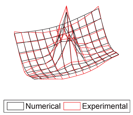
1. Introduction
The applications of sandwich structures continue to increase rapidly and range from satellites, spacecrafts, aircrafts, ships, automobiles, rail cars, wind energy systems to bridge construction, among others [1]. Sandwich panels typically consist of two thin face sheets or skins and a lightweight thicker core, which is sandwiched between two faces to obtain a structure of superior bending stiffness. Nevertheless, due to manufacturing defects or impact loads, these structures can experience imperfect bonding or debonding between the skin and the honeycomb core. Debonding in a sandwich structure may severely degrade its mechanical properties, which can produce a catastrophic failure of the overall structure. Therefore, it is important to detect the presence of debonding at an early stage.
A disadvantage of sandwich structures is that their structural failures, especially in the core, cannot always be detected by traditional non-destructive detection methods. A global technique called vibration-based damage detection has been rapidly expanding over the last few years [2]. The basic idea is that vibration characteristics (natural frequencies, mode shapes, damping, frequency response function, etc.) are functions of the physical properties of the structure. Thus, changes to the material and/or geometric properties due to damage will cause detectable changes in the vibrations characteristics. A debonded region in a sandwich structure is equivalent to a delamination in composite laminates. Many studies have demonstrated that vibration characteristics are sensitive to delamination even if the delamination is located in hidden or internal areas [3,4]. Nevertheless, there have only been a few studies related to the debonding of sandwich structures [5–10].
Vibration-based damage assessment methods are classified as model-based or non-model based. Non-model-based methods detect damage by comparing the measurements from the undamaged and damaged structures, whereas model-based methods locate and quantify damage by correlating an analytical model with test data from a damaged structure. Additionally, model-based methods are particularly useful for predicting the system response to new loading conditions and/or new system configurations (damage states), allowing damage prognosis [11]. Model-based damage assessment requires the solution of a nonlinear inverse problem, which can be accomplished using supervised learning algorithms as neural networks or by global optimisation algorithms. The most successful applications of vibration-based damage assessment are model updating methods based on global optimization algorithms [12–16]. Nevertheless, these algorithms are exceedingly slow and the damage assessment process is achieved via a costly and time-consuming inverse process, which presents an obstacle for real-time health monitoring applications.
Supervised learning algorithms are an alternative to model updating. The objective of supervised learning is to estimate the structure’s health based on current and past samples. Supervised learning can be divided into two classes: parametric and non-parametric. Parametric approaches assumed a statistical model for the data samples. A popular parametric approach is to model each class density as Gaussian [17]. Nonparametric algorithms do not assume a structure for the data. The most frequently nonparametric algorithms used in damage assessment are artificial neural networks [18–24]. A trained neural network can potentially detect, locate and quantify structural damage in a short period of time. Hence, it can be used for real-time damage assessment. Although once a neural network is already trained it can process data very quickly, the slow learning speed and the large number of parameters that need to be tuned within the training stage have been a major bottleneck in their application [25].
A new nonparametric method for supervised learning was presented by Gupta et al. [26,27]. This method generalized linear approximation by using the maximum-entropy (max-ent) principle [28] for statistical inference. A similar approach was adopted by Erkan [29] for semi-supervised learning problems, where a decision rule is to be learned from labelled and unlabeled data. By using max-ent methods, training is avoided and data is processed in a period of time that is comparable to the one of neural networks. In addition, it only requires one parameter to be selected. Hence, max-ent methods become very appealing for real-time health monitoring applications. Gupta [26] demonstrated the application of the max-ent approach to color management and gas pipeline integrity problems. In the present paper, we demonstrate the applicability of max-ent methods in structural damage assessment.
The primary contribution of this research is the development of a real-time damage assessment algorithm for honeycomb panels that uses a linear approximation method in conjunction with the mode shapes and natural frequencies of the structure. The linear approximation is handled by a statistical inference model based on the maximum-entropy principle [28]. The honeycomb panels are modeled with finite elements using a simplified three-layer shell model. The adhesive layer between the skin and core is modeled using linear springs, with reduced rigidities for the debonded sectors. The algorithm is validated using experimental data from an aluminum honeycomb panel containing different damage scenarios.
The remainder of this work is structured as follows: Section 2 introduces the proposed damage assessment algorithm and provides previous research on the max-ent linear approximation method. Section 3 describes the construction of the numerical model for the honeycomb sandwich panel. Section 4 presents the experimental structure and the correlation between the experimental and numerical modes. Section 5 describes the setting up of the database. Section 6 presents the case studies and the damage assessment results. Finally, conclusions and forthcoming work are presented in Section 7.
2. Damage Assessment Using Linear Approximation with Maximum Entropy
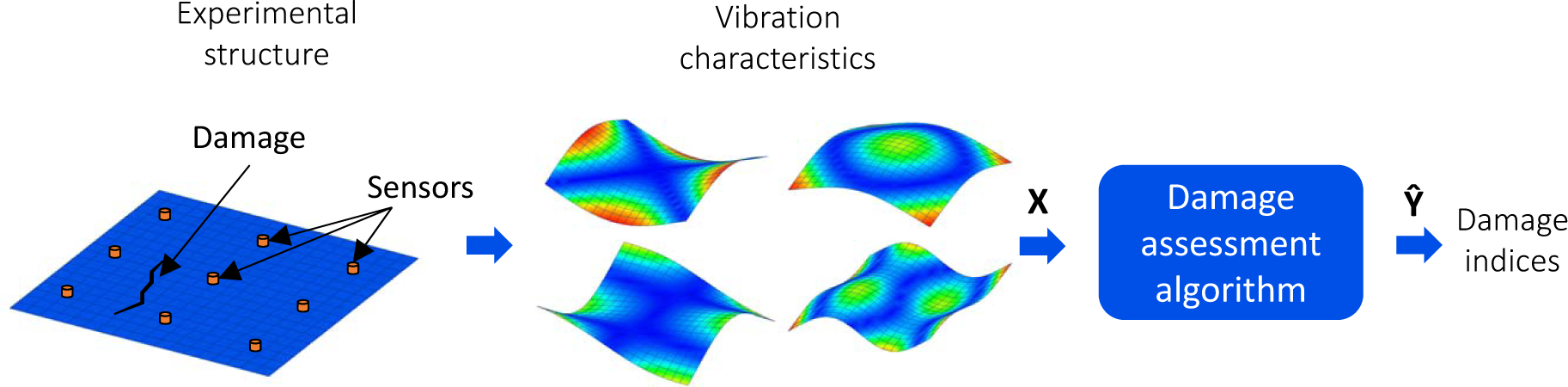
The main problem of vibration-based damage assessment is to ascertain the presence, location and severity of structural damage given a structure’s dynamic characteristics. This principle is illustrated in Figure 1; the vibration characteristics of the structure, which in this case correspond to mode shapes and natural frequencies, act as the input to the algorithm, and the outputs are the damage indices of each element in the structure.
Let the observation vector represent the ith damage state of the structure. Let the feature vector represent a set of vibration characteristics of the structure associated with the damage state Yi. The variables X and Y have joint distribution PX,Y. Let a set of k independent and identically distributed samples be drawn from PX,Y. These sample represent the database (X1, Y1), (X2, Y2), …, (Xk, Yk). The central problem in supervised learning is to form an estimate of PY|X, i.e. given a certain feature X, estimate the corresponding observation Y. Let Ŷ denote the estimated value of Y.
Linear approximation takes the N nearest neighbors to a test point X and uses a linear combination of them to represent X as
where w1, w2, …,wN are weighting functions, and X1(X), X2(X), …, XN(X) are the N closest neighbors to a test point X out of the database set. The equations given in (1) can be expressed as the following system of linear equations:

After w is obtained from Equation (2), Ŷ is estimated as
where Y1(X), Y2(X), …, YN(X) are the corresponding observations to the N selected neighbors. Typically, the system of Equation (2) is undetermined, and its solution is tackled via a constrained optimization technique of the family of least-squares (nonnegative least-squares [30]). An alternative that provides the least-biased solution is obtained via the maximum-entropy (max-ent) variational principle [28]. Recently, max-ent methods have become quite popular in the computational mechanics community as a powerful tool for numerical solution of PDEs [31–39], and their applications in the solution of ill-posed inverse problems have also been explored [40,41].
The notion of entropy in information theory was introduced by Shannon as a measure of uncertainty [42]. Later, on using the Shannon entropy, Jaynes [28] postulated the maximum-entropy principle as a rationale means for least-biased statistical inference when insufficient information is available. The maximum-entropy principle is suitable to find the least-biased probability distribution when there are fewer constraints than unknowns and is posed as follows:
Consider a set of N discrete events {x1, …, xN}. The possibility of each event is pi = p(xi) ∈ [0, 1] with uncertainty − ln pi. The Shannon entropy is the amount of uncertainty represented by the distribution {p1, …, pN}. The least-biased probability distribution and the one that has the most likelihood to occur is obtained via the solution of the following optimization problem (maximum-entropy principle):
subject to the constraints:
where is the non-negative orthant and < gr(x) > is the known expected value of functions gr(x) (r = 0, 1, …, m), with g0(x) = 1 being the normalizing condition.
The optimization problem (4) assigns probabilities to every xi in the set. Now, assume that the probability pi has an initial guess mi known as a prior, which reduces its uncertainty to − ln pi+ln mi = − ln(pi/mi). An alternative problem can be formulated by using this prior in (4) [43]:
subject to the constraints:
In (5), the variational principle associated with is known as the principle of minimum relative (cross) entropy [44,45]. Depending upon the prior employed, the optimization problem (5) will favor some xi in the set by assigning more probability to them, and eventually, assigning non-zero probability (pi > 0) to a selected number of xi (i < N) in the set. It can be easily seen that if the prior is constant, the Shannon-Jaynes entropy functional (4) is recovered as a particular case.
Because of its general character and flexibility, we adopt the relative entropy approach for our problem, where the probability pi is replaced with the weighting function wi of the linear approximation problem posed in Equation (1). This reads:
subject to the constraints:
where has been introduced as a shifted measure for stability purposes. A typical prior distribution is the smooth Gaussian [31]
where is a parameter that controls the radius of the Gaussian prior at Xi, and therefore its associated weight function; and hi is a characteristic n–dimensional Euclidean distance between neighbors that can be distinct for each Xi. In view of the optimization problem posed in (6) for supervised learning, maximizing the entropy chooses the weight solution that commits the least to any one in the database samples [27].
The solution of the max-ent optimization problem is handled by using the procedure of Lagrange multipliers, which yields [43]:
where .
In Equation (8), the Lagrange multiplier vector λ∗ is the minimizer of the dual optimization problem posed in Equation (6) [43]:
which gives rise to the following system of nonlinear equations:
where ∇λ stands for the gradient with respect to λ. Once the converged λ∗ is found, the weight functions are computed from Equation (8).
3. Numerical Model
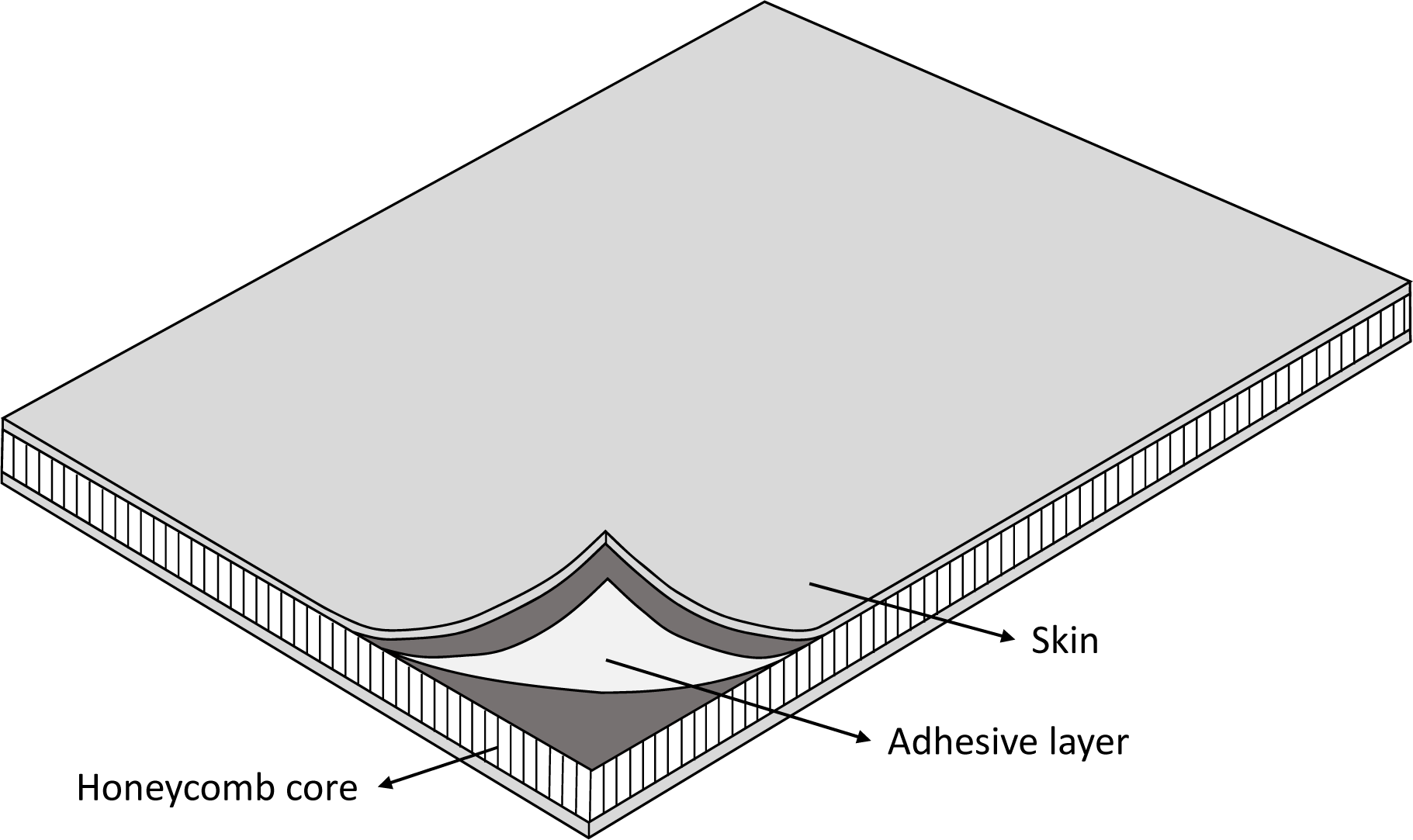
Figure 2 shows a scheme for a honeycomb sandwich panel, consisting of two thin face sheets or skins and a honeycomb core, which are bonded together by an adhesive layer. The panel can be modeled by a detailed 3D finite element model, but the computational effort increases very rapidly as the number of cells increases. Therefore, it is more convenient to develop equivalent simplified models for the honeycomb core to reduce the required computational time. Burton and Noor [46] studied the performance of nine different modeling approaches based on two-dimensional shell theories to predict the static response of sandwich panels. The results were compared to those from a detailed three-dimensional model. Their study showed that the global response can be accurately predicted by discrete three-layer models, predictor-corrector approaches and even first-order shear deformation theory, provided that proper values for the shear correction factors are used. According to Birman and Bert [47], a key factor in the practical application of the first-order shear deformation theory is the determination of the shear correction factor. The analysis presented by these researchers concluded that the shear correction factor should be taken with a value equal to unity for sandwich structures, as a first approximation. The work presented by Burton and Noor [48] showed that continuum layer models for the honeycomb core provide solutions that are close to those calculated by using detailed finite element models. Tanimoto et al. [49] used beam elements to model the honeycomb core and the adhesive layer. The proposed model was validated by experimental vibration tests. Burlayenko and Sadowski [50] performed an analysis of sandwich plates with hollow and foam-filled honeycomb cores using a commercially available finite element code. The sandwich plates were modeled on the basis of a simplified three-layered continuum model using a mixed shell/solid approach.
Consequently, the prediction of the dynamic response of the honeycomb panels can be accomplished by equivalent continuum models. In the present study, the honeycomb panels are modeled with finite elements using a simplified three-layer shell model and the adhesive layer between the skin and core is modeled using linear springs. Because the properties of the skin are known, the attention is focused on modeling the effective properties of the adhesive layer and the core material.
A debonded region between the skin and core of a honeycomb panel is similar to a delamination in laminated composites. There are a considerable amount of analytical and numerical methods used to model delaminated composite laminates. Della and Shu [51] provided an extensive review of them. The majority of these methods can be categorized into two classes. The first is a region approach where the laminate is divided into sub-laminates and continuity conditions are imposed at the junctions, whereas the second is a layer-wise model where delamination is introduced as an embedded layer or as a discontinuity function in the displacement field. On the other hand, modeling vibrations in sandwich structures with debonding is generally accompanied by contact problems between the interfaces of the debonded region [52]. Burlayenko and Sadowski [7,8] modeled the debonded region by creating a small gap between the face and the core and by introducing bi-linear spring elements between the double nodes in the debonded area. The springs have a stiffness equal to zero in tension and a large value in compression, simulating a contact condition. A piecewise-linear model does not predict a unique mode shape as in a linear system, but the mode shape depends on the vibration amplitude.
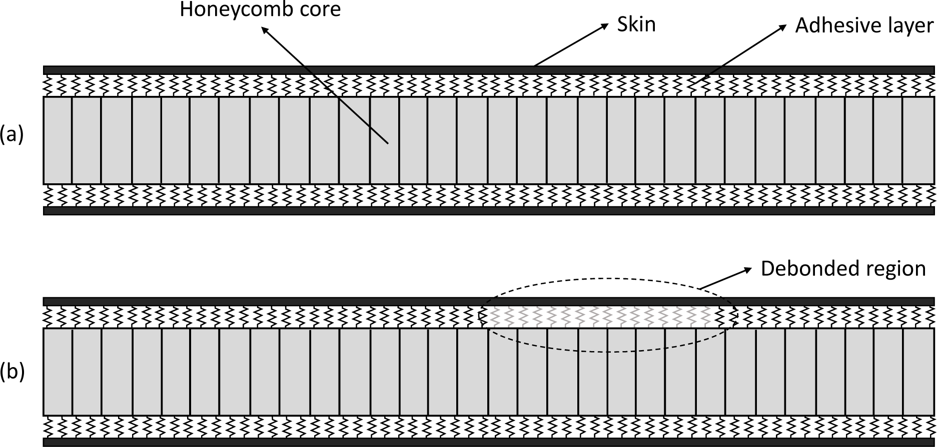
In this study, the adhesive layer between the skin and core is modeled using linear springs, with reduced rigidity in debonded sectors, as shown in Figure 3.
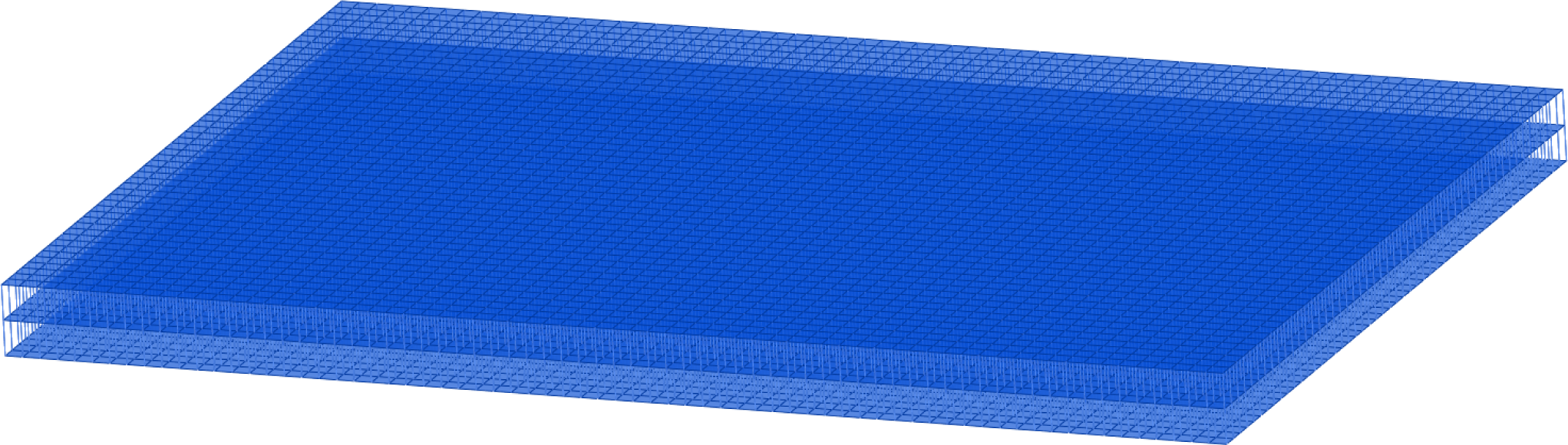
The numerical model is built in Matlab® using the SDTools Structural Dynamics Toolbox [53], the skins and honeycomb panel are modeled with standard isotropic 4-node shell elements. The final model shown in Figure 4 has 10,742 shell and 7,242 spring elements. The mechanical properties of the sandwich construction depend upon the adhesives, temperature and pressure used during curing. In addition, the anisotropic nature of the honeycomb core makes testing the sandwich specimens mandatory to determine their properties with accuracy. Here, the mechanical properties of the adhesive layer and the honeycomb core are determined by updating the finite element model with the experimental mode shapes and natural frequencies for both undamaged cases and those with debonding.
4. Experimental structure
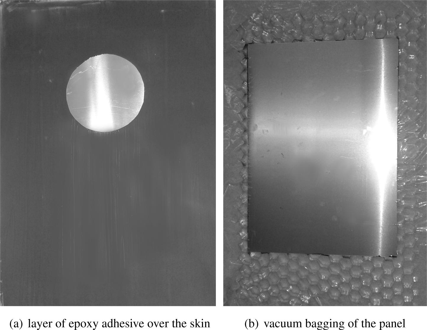
The experimental structure consists of a sandwich panel of 0.25 × 0.35 m2 made of an aluminum honeycomb core bonded to two aluminum skins, each with a thickness of 0.8 mm. The properties of the core are summarized in Table 1. The skins are bonded to the honeycomb core using an epoxy adhesive that provides a high performance solution to ambient temperature cure bonding of aluminum honeycomb to a wide range of skin materials. Figure 5a shows an aluminum sheet with a layer of epoxy adhesive, the circular region without adhesive is introduced to simulate debonding. Damaged panels were build with circular-shaped debonded regions with radius between 0.038 m and 0.045 m. To ensure perfect bonding, the panel is cured using a vacuum bagging system, as shown in Figure 5b.
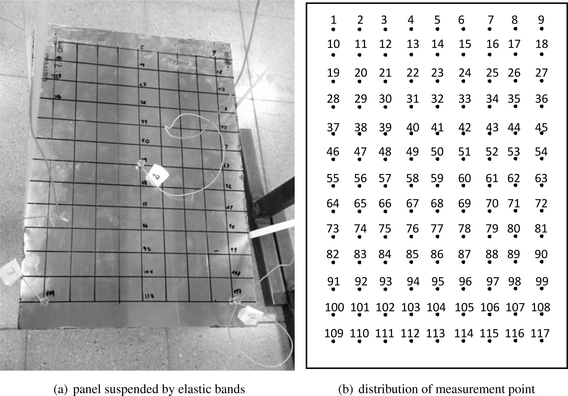
Figure 6 shows the experimental setup used to simulate a free boundary condition. The honeycomb sandwich panel is suspended by soft elastic bands. The out of plane vibration is captured by four miniature piezoelectric accelerometers located in three corners and in the centre of the panel. The panel is excited by an impact hammer at the 117 points described in Figure 6b, resulting in 468 measured Frequency Response Functions.
The identified modal parameters of the experimental structure are used to update the numerical model. The parameters that were updated in the numerical model are the following: the density and Young’s Modulus of the skins; the density, bending stiffness and shear correction factor of the core; and the stiffness of the springs representing the adhesive layer. The updated parameters are presented in Table 2.
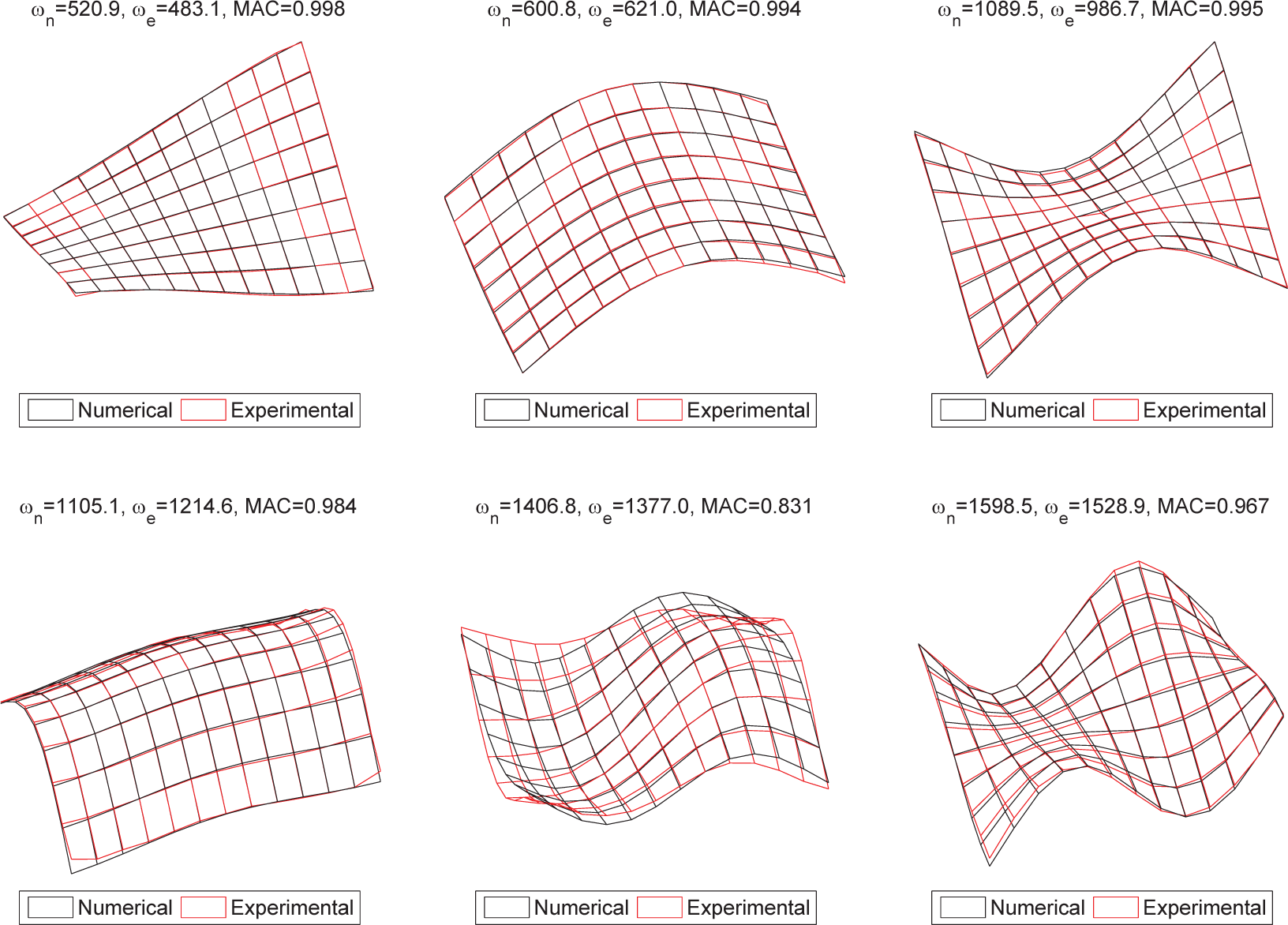
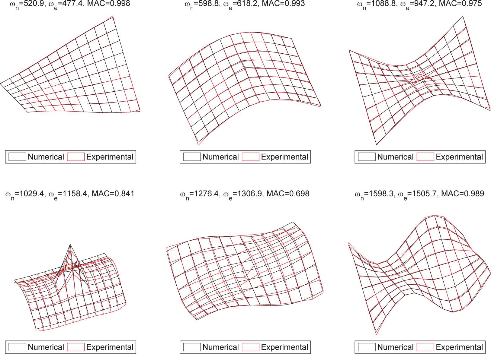
Figure 7 shows the first six experimental mode shapes compared to those from the numerical model after updating. The correlation between two mode shapes is measured by the Modal Assurance Criterion (MAC), defined as,
Where φi is the ith mode shape, subscripts N, E refer to numerical and experimental respectively. A MAC value of 0 indicates no correlation whereas a value of 1 indicates two completely correlated modes.
The results show that the correlation between the numerical and experimental modes is almost perfect for the first three modes, with MAC values higher than 0.99. The fifth mode presents the lowest correlation, with a MAC value of 0.83. In this case, the first-order shear approximation may not be sufficient. The maximum difference between the experimental and the numerical natural frequencies is 11%.
Figure 8 presents the correlation between the numerical and experimental global modes for the case with a circular debonded region at the centre of the plate. The modes are plotted over the surface of the debonded skin. Here, the numerical model was updated again considering the spring stiffness in the debonded region as updating parameter. Although the correlation is not as good as in the undamaged case, both the numerical and experimental models show the same behavior in the presence of damage, which is a reduction in the natural frequencies, and a strong discontinuity at the debonded region for mode 4.
5. Construction of the Database
The database is built as follows:
- (1)
Define a set of damage scenarios to be used in the database.
- (2)
Set j = 1.
- (3)
Parameterized the jth scenario with an observation vector Yj.
- (4)
Build the numerical model associated with the jth scenario.
- (5)
Construct a feature vector Xj using the modal parameters derived from the numerical model.
- (6)
Add the pair of vectors (Xj, Yj) to the database, set j = j + 1 and go to step 3.
The damage scenarios used to construct the database consist of panels with circular-shaped debonded regions at one of the 117 points that are depicted in Figure 6b. Debonding is restricted to the skin that is measured during experiments. For each of the 117 points, thirteen debonded radius between 0.01 m and 0.07 m are considered (i.e. 0.01, 0.015, …, 0.065, 0.07) resulting in 1521 pairs of vectors in the database. The next subsections describe how the observation and feature vectors are built.
5.1. Observation Vector
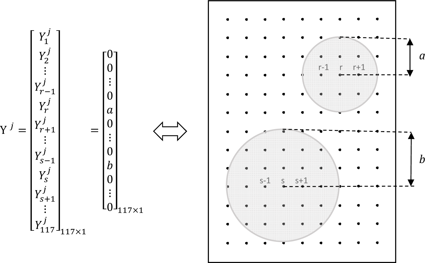
Damage is modeled by circular-shaped debonded regions centered at some of the 117 points that are shown in Figure 6b. The jth observation vector is , where the value implies a debonded region that extends to a radius from the ith point. Figure 9 illustrates an example of an observation vector Yj that represents a damage scenario with two debonded regions centered at points r and s.
5.2. Feature Vector
The first six global mode shapes and natural frequencies that are shown in Figure 7 are used to build the feature vectors. The jth feature vector Xj contains the experimental changes in the natural frequencies and mode shapes with respect to the intact case:

where ω represents a vector that contains the natural frequencies and ϕj represents the ith mode shape vector. The superscripts D and U refer to damaged and undamaged, respectively. The vector of the mode shape changes is normalized with respect to its maximum value to reduce the difference between the numerical and experimental results. This difference is expected because the numerical model does not contain contact conditions whereas the experimental model does.
Since each mode shape is a vector of dimension 117 × 1 and each vector of natural frequencies has dimension 6×1, the feature vectors have dimension 123×1. A disadvantage of high-dimensional feature spaces, as the present case, is that points that are scattered in those spaces are usually far from each other. Thus, neighborhood methods that are based purely on distance become less useful. Nevertheless, Gupta [26] showed that the linear approximation with maximum entropy is more suited than standard neighborhood methods for three and higher dimension feature spaces.
6. Damage Assessment Results
The algorithm is tested for the three experimental damage scenarios shown in Figure 10. The first case has a debonded region centered at point 59 (the centre of the panel), the second case has a debonded region centered nearby points 30, 31, 39 and 40, and the third case has a debonded region centered nearby points 31, 32, 40, 41. The radius for the three debonded regions are 0.038 m, 0.039 m and 0.045 m respectively. Debonding was introduced into the experimental panels by purposely leaving circular areas without adhesive as shown in Figure 5a.
The results of the max-ent linear approximation algorithm are compared with those obtained by solving the nonnegative least-squares problem posed in Equation (2). The procedure to assess the experimental damage using both approaches is implemented as follows:
- (1)
Perform an experimental modal analysis of the damaged panel and identify the first six global mode shapes and natural frequencies.
- (2)
Construct the feature test point X using Equation (12).
- (3)
Read the feature vectors in the database.
- (4)
Compute weights.
Max-ent
- (a)
Select parameter βi in the Gaussian prior given in Equation (7), so that k neighbors contribute to the solution.
- (b)
Solve the system of nonlinear equations presented in Equation (10).
- (c)
Compute the weight functions from Equation (8).
Nonnegative least-squares
- (a)
Select the k closest neighbors.
- (b)
Build the matrices A and b in Equation (2).
- (c)
Compute the weights using the Matlab function lsqnonneg.
- (5)
Read the observation vectors in the database and estimate the experimental damage from (3).
Both methods use the ten closest neighbors to the test point. The time needed to solve the linear approximation problem (stages 4 and 5 above) is 0.7 and 0.03 seconds for the max-ent and nonnegative least-squares approaches, respectively. Table 3 details the running time of both algorithms. It is clear that a more efficient method to select the parameter βi could greatly reduce the computational time of the max-ent approach. Nevertheless, it should be noted that both algorithms can reach a solution in less than a second, which can be considered real-time for structural damage assessment problems. Other algorithms such as parallel genetic algorithms can take between 1000 and 10000 seconds to solve a similar problem [12].
Figures 11, 12 and 13 present the damage assessment results. In these figures, the black zones indicate the detected damage, where each pixel represents a debonded spring. The actual damage introduced into the panel is depicted by a circle. In the three cases, the max-ent approach identifies debonded regions that are closer to the actual damage than those identified by the least-squares method. In the first case, the centre of the experimental damage matches one of the 117 predefined locations. Thus, the max-ent algorithm is able to detect the exact location of the debonded region. However, when the actual centre of the damage does not match one of the 117 locations, as in the second and third cases, the algorithm detects the damage at a location that is close to the actual location but not at the exact location.
7. Conclusions and Further Research
This article presented a new methodology to identify debonded regions in aluminum honeycomb panels using a linear approximation method handled by a statistical inference model based on the maximum-entropy principle. The algorithm was validated using experimental data from an aluminum honeycomb panel subjected to different damage scenarios.
The honeycomb panels were modeled with finite elements using a simplified three-layer shell model. The adhesive layer between the skin and core was modeled using linear springs with the rigidity being reduced at debonded locations. This numerical model predicted the first six modes of the undamaged and damaged panels with reasonable accuracy. Nevertheless, the numerical model can be improved by using higher order shear approximations.
In the three experimental cases, the linear approximation using the max-ent technique was successful in assessing the experimental damage. The detected damage closely corresponds with the experimental damage in all cases. In addition, the damage state of the panels is assessed in less than one second thereby providing the possibility of real-time damage assessment.
The results show that the proposed algorithm can assess debonded regions with sizes between 0.038 m and 0.045 m. It would be useful to establish the minimum size that can be detected with confidence. This value largely depends on the sensitivity of mode shapes and natural frequencies to damage and on the level of experimental variability.
The proposed damage assessment algorithm provides only two options for a spring in the adhesive layer: either healthy or debonded. This can be improved by setting the output for each spring as a number associated with a debonding probability that ranges from 0 to 1.
Lastly, further research is needed to adapt this algorithm to cases with multiple debonded regions and to test its performance in more realistic configurations than a free plate.
Acknowledgments
Valentina del Fierro was supported by CONICYT grant CONICYT-PCHA/Magster Nacional/2013-221320691. The authors acknowledge the partial financial support of the Chilean National Fund for Scientific and Technological Development (Fondecyt) under Grants No. 11110389 and 11110046.
Author Contributions
Viviana Meruane and Valentina del Fierro built the updated numerical model, designed the experiment, processed and analyzed the experimental data, and tested the damage assessment algorithm. Alejandro Ortiz-Bernardin programmed the max-ent linear approximation algorithm and adapted it to the application case. The article was written by Viviana Meruane and Alejandro Ortiz-Bernardin.
Conflicts of Interest
The authors declare no conflict of interest
References
- Vinson, J.R. Sandwich structures: past, present, and future. In Sandwich Structures 7: Advancing with Sandwich Structures and Materials; Springer: Dordrecht, The Netherlands, 2005; pp. 3–12. [Google Scholar]
- Carden, E.; Fanning, P. Vibration Based Condition Monitoring: A Review. Struct. Health Monit 2004, 3, 355–377. [Google Scholar]
- Zou, Y.; Tong, L.; Steven, G. Vibration-based model-dependent damage (delamination) identification and health monitoring for composite structures-a review. J. Sound Vib 2000, 230, 357–378. [Google Scholar]
- Montalvao, D.; Maia, N.; Ribeiro, A. A. Review of Vibration-based Structural Health Monitoring with Special Emphasis on Composite Materials. Shock Vib. Digest 2006, 38, 295–324. [Google Scholar]
- Jiang, L.; Liew, K.; Lim, M.; Low, S. Vibratory behaviour of delaminated honeycomb structures: A 3-D finite element modelling. Comput. Struct 1995, 55, 773–788. [Google Scholar]
- Kim, H.Y.; Hwang, W. Effect of debonding on natural frequencies and frequency response functions of honeycomb sandwich beams. Compos. Struct 2002, 55, 51–62. [Google Scholar]
- Burlayenko, V.; Sadowski, T. Dynamic behaviour of sandwich plates containing single/multiple debonding. Comput. Mater. Sci 2011, 50, 1263–1268. [Google Scholar]
- Burlayenko, V.N.; Sadowski, T. Influence of skin/core debonding on free vibration behavior of foam and honeycomb cored sandwich plates. Int. J. Non-Lin. Mech 2010, 45, 959–968. [Google Scholar]
- Mohanan, A.; Pradeep, K.; Narayanan, K. Performance Assessment of Sandwich Structures with Debonds and Dents. Int. J. Sci. Eng. Res 2013, 4, 174–179. [Google Scholar]
- Shahdin, A.; Morlier, J.; Gourinat, Y. Damage monitoring in sandwich beams by modal parameter shifts: A comparative study of burst random and sine dwell vibration testing. J. Sound Vib 2010, 329, 566–584. [Google Scholar]
- Farrar, C.; Lieven, N. Damage prognosis: the future of structural health monitoring. Philos. Trans. A Math. Phys. Eng. Sci 2007, 365, 623–632. [Google Scholar]
- Meruane, V.; Heylen, W. Damage detection with parallel genetic algorithms and operational modes. Struct. Health Monit 2010, 9, 481–496. [Google Scholar]
- Meruane, V.; Heylen, W. An hybrid real genetic algorithm to detect structural damage using modal properties. Mech. Syst. Signal Process 2011, 25, 1559–1573. [Google Scholar]
- Perera, R.; Torres, R. Structural damage detection via modal data with genetic algorithms. J. Struct. Eng 2006, 132, 1491–1501. [Google Scholar]
- Kouchmeshky, B.; Aquino, W.; Bongard, J.; Lipson, H. Co-evolutionary algorithm for structural damage identification using minimal physical testing. Int. J. Numer. Meth. Eng 2007, 69, 1085–1107. [Google Scholar]
- Teughels, A.; De Roeck, G.; Suykens, J. Global optimization by coupled local minimizers and its application to FE model updating. Comput. Struct 2003, 81, 2337–2351. [Google Scholar]
- Markou, M.; Singh, S. Novelty detection: a review–part 1: statistical approaches. Signal Process 2003, 83, 2481–2497. [Google Scholar]
- Islam, A.S.; Craig, K.C. Damage detection in composite structures using piezoelectric materials (and neural net). Smart Mater. Struct 1994, 3, 318–328. [Google Scholar]
- Okafor, A.C.; Chandrashekhara, K.; Jiang, Y. Delamination prediction in composite beams with built-in piezoelectric devices using modal analysis and neural network. Smart Mater. Struct 1996, 5, 338–347. [Google Scholar]
- Valoor, M.T.; Chandrashekhara, K. A thick composite-beam model for delamination prediction by the use of neural networks. Compos. Sci. Tech 2000, 60, 1773–1779. [Google Scholar]
- Ishak, S.; Liu, G.; Shang, H.; Lim, S. Locating and sizing of delamination in composite laminates using computational and experimental methods. Compos. B Eng 2001, 32, 287–298. [Google Scholar]
- Chakraborty, D. Artificial neural network based delamination prediction in laminated composites. Mater. Des 2005, 26, 1–7. [Google Scholar]
- Su, Z.; Ling, H.Y.; Zhou, L.M.; Lau, K.T.; Ye, L. Efficiency of genetic algorithms and artificial neural networks for evaluating delamination in composite structures using fibre Bragg grating sensors. Smart Mater. Struct 2005, 14, 1541–1553. [Google Scholar]
- Zhang, Z.; Shankar, K.; Ray, T.; Morozov, E.V.; Tahtali, M. Vibration-Based Inverse Algorithms for Detection of Delamination in Composites. Compos. Struct 2013, 102, 226–236. [Google Scholar]
- Meruane, V.; Mahu, J. Real-time structural damage assessment using artificial neural networks and anti-resonant frequencies. Shock Vib 2014, 2014, 653279:1–653279:14. [Google Scholar]
- Gupta, M.R. An information theory approach to supervised learning. PhD thesis, Stanford University, CA, USA, 2003. [Google Scholar]
- Gupta, M.R.; Gray, R.M.; Olshen, R.A. Nonparametric supervised learning by linear interpolation with maximum entropy. IEEE Trans. Pattern Anal. Mach. Intell 2006, 28, 766–781. [Google Scholar]
- Jaynes, E.T. Information theory and statistical mechanics. Phys. Rev 1957, 106, 620–630. [Google Scholar]
- Erkan, A.N. Semi-supervised learning via generalized maximum entropy. PhD thesis, New York University, NY, USA, 2010. [Google Scholar]
- Lawson, C.L.; Hanson, R.J. Solving least squares problems; SIAM: New Jersey, USA, 1974; pp. 161–164. [Google Scholar]
- Arroyo, M.; Ortiz, M. Local maximum-entropy approximation schemes: A seamless bridge between finite elements and meshfree methods. Int. J. Numer. Meth. Eng 2006, 65, 2167–2202. [Google Scholar]
- Ortiz, A.; Puso, M.A.; Sukumar, N. Maximum-entropy meshfree method for compressible and near-incompressible elasticity. Comput. Meth. Appl. Mech. Eng 2010, 199, 1859–1871. [Google Scholar]
- Yaw, L.L.; Sukumar, N.; Kunnath, S.K. Meshfree co-rotational formulation for two-dimensional continua. Int. J. Numer. Meth. Eng 2009, 79, 979–1003. [Google Scholar]
- Cyron, C.J.; Arroyo, M.; Ortiz, M. Smooth, second order, non-negative meshfree approximants selected by maximum entropy. Int. J. Numer. Meth. Eng 2009, 79, 1605–1632. [Google Scholar]
- Rosolen, A.M.; Millán, R.D.; Arroyo, M. On the optimum support size in meshfree methods: A variational adaptivity approach with maximum entropy approximants. Int. J. Numer. Meth. Eng 2010, 82, 868–895. [Google Scholar]
- González, D.; Cueto, E.; Doblaré, M. A higher order method based on local maximum entropy approximation. Int. J. Numer. Meth. Eng 2010, 83, 741–764. [Google Scholar]
- Li, B.; Habbal, F.; Ortiz, M. Optimal transportation meshfree approximation schemes for fluid and plastic flows. Int. J. Numer. Meth. Eng 2010, 83, 1541–1579. [Google Scholar]
- Cyron, C.; Nissen, K.; Gravemeier, V.; Wall, W. Stable meshfree methods in fluid mechanics based on Green’s functions. Comput. Mech 2010, 46, 287–300. [Google Scholar]
- Cyron, C.; Nissen, K.; Gravemeier, V.; Wall, W. Information flux maximum-entropy approximation schemes for convection and diffusion problems. Int. J. Numer. Meth. Fluid 2010, 64, 1180–1200. [Google Scholar]
- Gamboa, F.; Gassiat, E. Bayesian methods and maximum entropy for ill-posed inverse problems. Ann. Stat 1997, 25, 328–350. [Google Scholar]
- Loubes, J.M.; Pelletier, B. Maximum entropy solution to ill-posed inverse problems with approximately known operator. J. Math. Anal. Appl 2008, 344, 260–273. [Google Scholar]
- Shannon, C.E. A mathematical theory of communication. Bell Syst. Tech. J 1948, 27, 379–423. [Google Scholar]
- Sukumar, N.; Wright, R.W. Overview and construction of meshfree basis functions: From moving least squares to entropy approximants. Int. J. Numer. Meth. Eng 2007, 70, 181–205. [Google Scholar]
- Kullback, S. Information Theory and Statistics; Wiley: New York, USA, 1959. [Google Scholar]
- Shore, J.E.; Johnson, R.W. Axiomatic derivation of the principle of maximum entropy and the principle of minimum cross-entropy. IEEE Trans. Inform. Theor 1980, 26, 26–36. [Google Scholar]
- Burton, W.S.; Noor, A.K. Assessment of computational models for sandwich panels and shells. Comput. Meth. Appl. Mech. Eng 1995, 124, 125–151. [Google Scholar]
- Birman, V.; Bert, C.W. On the choice of shear correction factor in sandwich structures. J. Sandw. Struct. and Mater 2002, 4, 83–95. [Google Scholar]
- Burton, W.; Noor, A. Assessment of continuum models for sandwich panel honeycomb cores. Comput. Meth. Appl. Mech. Eng 1997, 145, 341–360. [Google Scholar]
- Tanimoto, Y.; Nishiwaki, T.; Shiomi, T.; Maekawa, Z. A numerical modeling for eigenvibration analysis of honeycomb sandwich panels. Compos. Interfac 2001, 8, 393–402. [Google Scholar]
- Burlayenko, V.N.; Sadowski, T. Analysis of structural performance of sandwich plates with foam-filled aluminum hexagonal honeycomb core. Comput. Mater. Sci 2009, 45, 658–662. [Google Scholar]
- Della, C.N.; Shu, D. Vibration of delaminated composite laminates: A review. Appl. Mech. Rev 2007, 60, 1–20. [Google Scholar]
- Müller, I. Clapping in delaminated sandwich-beams due to forced oscillations. Comput. Mech 2007, 39, 113–126. [Google Scholar]
- SDTools, Structural dynamics toolbox & FEMLink. Users Guide Version; SDTools: Paris, France, 2014.


| Property | Value |
|---|---|
| Cell size | 19.1 mm |
| Foil thickness | 5 × 10⁻⁵ m |
| Thickness | 10 mm |
| Density | 20.8 kg/m3 |
| Compressive strength | 0.448 MPa |
| Shear strength in longitudinal direction (σxy) | 0.345 MPa |
| Shear modulus in longitudinal direction (Gxy) | 89.63 MPa |
| Shear strength in width direction (σyz) | 0.241 MPa |
| Shear modulus in width direction (Gyz) | 41.37 MPa |
| Component | Property | Value |
|---|---|---|
| Skin | Density | 2.53 × 10³ kg/m3 |
| Young’s modulus | 6.14 × 10¹⁰ Pa | |
| Core | Density | 31.1 kg/m3 |
| Young’s modulus | 2.41 × 10¹⁰ Pa | |
| Shear correction factor | 0.67 | |
| Adhesive layer | Stiffness healthy layer | 3.42 × 10⁸ Nm−1/m2 |
| Stiffness debonded layer | 4.96 × 10⁷ Nm−1/m2 | |
| Stage | Time (s) | ||
|---|---|---|---|
| Max-ent | Nonnegative least-squares | ||
| 4 | (a) | 5.91×10⁻¹ | 4.30×10⁻³ |
| (b) | 9.89×10⁻² | 1.24×10⁻⁴ | |
| (c) | 1.00×10⁻² | 2.90×10⁻³ | |
| 5 | 8.7×10⁻⁵ | 8.7×10⁻⁵ |
© 2014 by the authors; licensee MDPI, Basel, Switzerland This article is an open access article distributed under the terms and conditions of the Creative Commons Attribution license (http://creativecommons.org/licenses/by/3.0/).
Share and Cite
Meruane, V.; Fierro, V.D.; Ortiz-Bernardin, A. A Maximum Entropy Approach to Assess Debonding in Honeycomb aluminum Plates. Entropy 2014, 16, 2869-2889. https://doi.org/10.3390/e16052869
Meruane V, Fierro VD, Ortiz-Bernardin A. A Maximum Entropy Approach to Assess Debonding in Honeycomb aluminum Plates. Entropy. 2014; 16(5):2869-2889. https://doi.org/10.3390/e16052869
Chicago/Turabian StyleMeruane, Viviana, Valentina Del Fierro, and Alejandro Ortiz-Bernardin. 2014. "A Maximum Entropy Approach to Assess Debonding in Honeycomb aluminum Plates" Entropy 16, no. 5: 2869-2889. https://doi.org/10.3390/e16052869