Information-Geometric Markov Chain Monte Carlo Methods Using Diffusions

Abstract
: Recent work incorporating geometric ideas in Markov chain Monte Carlo is reviewed in order to highlight these advances and their possible application in a range of domains beyond statistics. A full exposition of Markov chains and their use in Monte Carlo simulation for statistical inference and molecular dynamics is provided, with particular emphasis on methods based on Langevin diffusions. After this, geometric concepts in Markov chain Monte Carlo are introduced. A full derivation of the Langevin diffusion on a Riemannian manifold is given, together with a discussion of the appropriate Riemannian metric choice for different problems. A survey of applications is provided, and some open questions are discussed.1. Introduction
There are three objectives to this article. The first is to introduce geometric concepts that have recently been employed in Monte Carlo methods based on Markov chains [1] to a wider audience. The second is to clarify what a “diffusion on a manifold” is, and how this relates to a diffusion defined on Euclidean space. Finally, we review the state-of-the-art in the field and suggest avenues for further research.
The connections between some Monte Carlo methods commonly used in statistics, physics and application domains, such as econometrics, and ideas from both Riemannian and information geometry [2,3] were highlighted by Girolami and Calderhead [1] and the potential benefits demonstrated empirically. Two Markov chain Monte Carlo methods were introduced, the manifold Metropolis-adjusted Langevin algorithm and Riemannian manifold Hamiltonian Monte Carlo. Here, we focus on the former for two reasons. First, the intuition for why geometric ideas can improve standard algorithms is the same in both cases. Second, the foundations of the methods are quite different, and since the focus of the article is on using geometric ideas to improve performance, we considered a detailed description of both to be unnecessary. It should be noted, however, that impressive empirical evidence exists for using Hamiltonian methods in some scenarios (e.g., [4]). We refer interested readers to [5,6].
We take an expository approach, providing a review of some necessary preliminaries from Markov chain Monte Carlo, diffusion processes and Riemannian geometry. We assume only a minimal familiarity with measure-theoretic probability. More informed readers may prefer to skip these sections. We then provide a full derivation of the Langevin diffusion on a Riemannian manifold and offer some intuition for how to think about such a process. We conclude Section 4 by presenting the Metropolis-adjusted Langevin algorithm on a Riemannian manifold.
A key challenge in the geometric approach is which manifold to choose. We discuss this in Section 4.4 and review some candidates that have been suggested in the literature, along with the reasoning for each. Rather than provide a simulation study here, we instead reference studies where the methods we describe have been applied in Section 5. In Section 6, we discuss several open questions, which we feel could be interesting areas of further research and of interest to both theorists and practitioners.
Throughout, π (·) will refer to an n-dimensional probability distribution and π (x) its density with respect to the Lebesgue measure.
2. Markov Chain Monte Carlo
Markov chain Monte Carlo (MCMC) is a set of methods for drawing samples from a distribution, π (·), defined on a measurable space , whose density is only known up to some proportionality constant. Although the i-th sample is dependent on the (i − 1)-th, the Ergodic Theorem ensures that for an appropriately constructed Markov chain with invariant distribution π (·), long-run averages are consistent estimators for expectations under π (·). As a result, MCMC methods have proven useful in Bayesian statistical inference, where often, the posterior density π(x|y) ∝ f (y|x)π0(x) for some parameter, x (where f (y|x) denotes the likelihood for data y and π0(x) the prior density), is only known up to a constant [7]. Here, we briefly introduce some concepts from general state space Markov chain theory together with a short overview of MCMC methods. The exposition follows [8].
2.1. Markov Chain Preliminaries
A time-homogeneous Markov chain, {Xm}m∈ℕ, is a collection of random variables, Xm, each of which is defined on a measurable space , such that:
for any . We define the transition kernel P(xm−1, A) = ℙ[Xm ∈ A|Xm−1 = xm−1] for the chain to be a map for which P(x, ·) defines a distribution over for any x ∈ , and P(·, A) is measurable for any . Intuitively, P defines a map from points to distributions in . Similarly, we define the m-step transition kernel to be:
We call a distribution π (·) invariant for {Xm}m∈ℕ if:
for all . If P(x, ·) admits a density, p(x′|x), this can be equivalently written:
The connotation of Equations (3) and (4) is that if Xm ~ π(·), then Xm+s ~ π(·) for any s ∈ ℕ. In this instance, we say the chain is “at stationarity”. Of interest to us will be Markov chains for which there is a unique invariant distribution, which is also the limiting distribution for the chain, meaning that for any for which π(x0) > 0:
for any . Certain conditions are required for Equation (5) to hold, but for all Markov chains presented here, these are satisfied (though, see [8]).
A useful condition, which is sufficient (though not necessary) for π(·) to be an invariant distribution, is reversibility, which can be shown by the relation:
Integrating over both sides with respect to x, we recover Equation (4). In other words, a chain is reversible if, at stationarity, the probability that xi ∈ A and xi+1 ∈ B are equal to the probability that xi+1 ∈ A and xi ∈ B. The relation (6) will be the primary tool used to construct Markov chains with a desired invariant distribution in the next section.
2.1.1. Monte Carlo Estimates from Markov Chains
Of most interest here are estimators constructed from a Markov chain. The Ergodic Theorem states that for any chain, {Xm}m∈ℕ, satisfying Equation (5) and any g ∈ L1(π), we have that:
with probability one [7]. This is a Markov chain analogue to the Law of large numbers.
The efficiency of estimators of the form can be assessed through the autocorrelation between elements in the chain. We will assess the efficiency of relative to estimators , where {Zi}m∈ℕ is a sequence of independent random variables, each having distribution π(·). Provided Varπ[g(Zi)] < ∞, then . We now seek a similar result for estimators of the form, .
It follows directly from the Kipnis–Varadhan Theorem [9] that an estimator, , from a reversible Markov chain for which X0 ~ π(·) satisfies:
provided that , where ρ(0,i) = Corrπ[g(X0), g(Xi)]. We will refer to the constant, τ, as the autocorrelation time for the chain.
Equation (8) implies that for large enough m, . In practical applications, the sum in Equation (8) is truncated to the first p − 1 realisations of the chain, where p is the first instance at which |ρ(0,p)| < ϵ for some ϵ > 0. For example, in the Convergence Diagnosis and Output Analysis for MCMC (CODA) package within the R statistical software ϵ = 0.05 [10,11].
Another commonly used measure of efficiency is the effective sample size meff = m/τ, which gives the number of independent samples from π(·) needed to give an equally efficient estimate for π[g(X)]. Clearly, minimising τ is equivalent to maximising meff.
The measures arising from Equation (8) give some intuition for what sort of Markov chain gives rise to efficient estimators. However, in practice, the chain will never be at stationarity. Therefore, we also assess Markov chains according to how far away they are from this point. For this, we need to measure how close Pm(x0, ·) is from π(·), which requires a notion of distance between probability distributions.
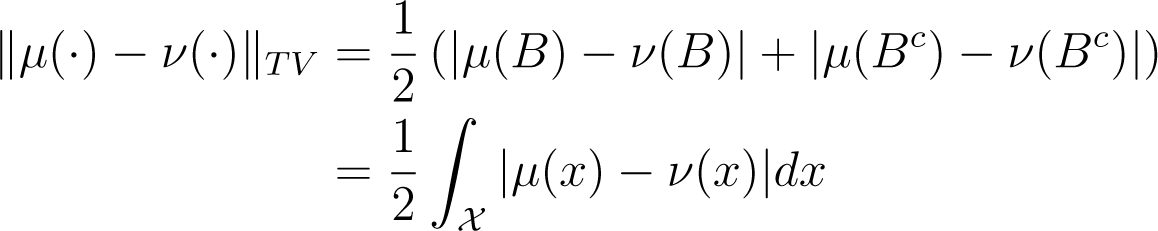
Although there are several appropriate choices [12], a common option in the Markov chain literature is the total variation distance:
which informally gives the largest possible difference between the probabilities of a single event in according to μ(·) and ν(·). If both distributions admit densities, Equation (9) can be written (see Appendix A):
which is proportional to the L1 distance between μ(x) and ν(x). Our metric, ‖ · ‖TV ∈ [0,1], with ‖ · ‖TV = 1 for distributions with disjoint supports and ‖μ(·) − ν(·)‖TV = 0, implies μ(·) ≡ ν(·).
Typically, for an unbounded , the distance ‖Pm(x0, ·) − π(·)‖TV will depend on x0 for any finite m. Therefore, bounds on the distance are often sought via some inequality of the form:
for some M < ∞, where depends on x0 and is called a drift function, and f: ℕ → [0, ∞) depends on the number of iterations, m (and is often defined, such that f (0) = 1).
A Markov chain is called geometrically ergodic if f (m) = rm in Equation (11) for some 0 < r < 1. If in addition to this, V is bounded above, the chain is called uniformly ergodic. Intuitively, if either condition holds, then the distribution of Xm will converge to π(·) geometrically quickly as m grows, and in the uniform case, this rate is independent of x0. As well as providing some (often qualitative if M and r are unknown) bounds on the convergence rate of a Markov chain, geometric ergodicity implies that a central limit theorem exists for estimators of the form, . For more detail on this, see [13,14].
In practice several approximate methods also exist to assess whether a chain is close enough to stationarity for long-run averages to provide suitable estimators (e.g., [15]). The MCMC practitioner also uses a variety of visual aids to judge whether an estimate from the chain will be appropriate for his or her needs.
2.2. Markov Chain Monte Carlo
Now that we have introduced Markov chains, we turn to simulating them. The objective here is to devise a method for generating a Markov chain, which has a desired limiting distribution, π(·). In addition, we would strive for the convergence rate to be as fast as possible and the effective sample size to be suitably large relative to the number of iterations. Of course, the computational cost of performing an iteration is also an important practical consideration. Ideally, any method would also require limited problem-specific alterations, so that practitioners are able to use it with as little knowledge of the inner workings as is practical.
Although other methods exist for constructing chains with a desired limiting distribution, a popular choice is the Metropolis–Hastings algorithm [7]. At iteration i, a sample is drawn from some candidate transition kernel, Q(xi−1, ·), and then either accepted or rejected (in which case, the state of the chain remains xi−1). We focus here on the case where Q(xi−1, ·) admits a density, q(x′|xi−1), for all xi−1 ∈ (though, see [8]). In this case, a single step is shown below (the wedge notation a ∧ b denotes the minimum of a and b). The “acceptance rate”, α(xi−1,x′), governs the behaviour of the chain, so that, when it is close to one, then many proposed moves are accepted, and the current value in the chain is constantly changing. If it is on average close to zero, then many proposals are rejected, so that the chain will remain in the same place for many iterations. However, α ≈ 1 is typically not ideal, often resulting in a large autocorrelation time (see below). The challenge in practice is to find the right acceptance rate to balance these two extremes.

| Require: xi−1 |
| Draw X′ ~ Q(xi−1, ·) |
| Draw Z ~ U[0, 1] |
| Set |
| if z < α(xi−1, x′) then |
| Set xi ← x′ |
| else |
| Set xi ← xi−1 |
| end if |
Combining the “proposal” and “acceptance” steps, the transition kernel for the resulting Markov chain is:
for any A ∈ B, where:
is the average probability that a draw from Q(x, ·) will be rejected, and δx(A) = 1 if x ∈ A and zero, otherwise. A Markov chain defined in this way will have π(·) as an invariant distribution, since the chain is reversible for π(·). We note here that:
in the case that the proposed move is accepted and that if the proposed move is rejected, then xi = xi−1; so the chain is reversible for π(·). It can be shown that π(·) is also the limiting distribution for the chain [7].
The convergence rate and autocorrelation time of a chain produced by the algorithm are dependent on both the choice of proposal, Q(xi−1, ·), and the target distribution, π(·). For simple forms of the latter, less consideration is required when choosing the former. A broad objective among researchers in the field is to find classes of proposal kernels that produce chains that converge and mix quickly for a large class of target distributions. We first review a simple choice before discussing one that is more sophisticated, and the will be the focus of the rest of the article.
2.3. Random Walk Proposals
An extremely simple choice for Q(x, ·) is one for which:
where ‖ · ‖ denotes some appropriate norm on , meaning the proposal is symmetric. In this case, the acceptance rate reduces to:
In addition to simplifying calculations, Equation (14) strengthens the intuition for the method, since proposed moves with higher density under π(·) will always be accepted. A typical choice for Q(x, ·) is , where the matrix, Σ, is often chosen in an attempt to match the correlation structure of π(·) or simply taken as the identity [16]. The tuning parameter, λ, is the only other user-specific input required.
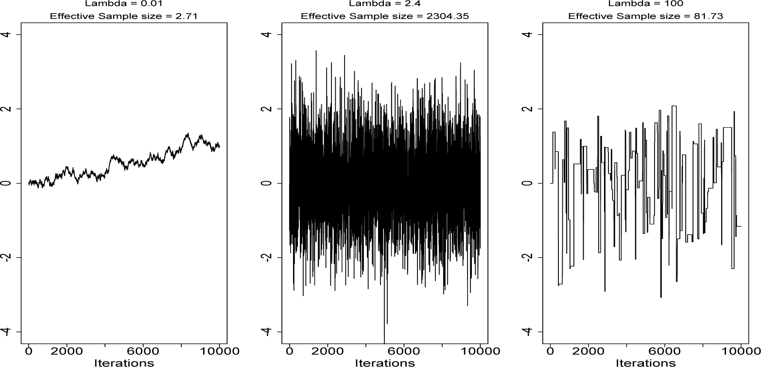
Much research has been conducted into properties of the random walk Metropolis algorithm (RWM). It has been shown that the optimal acceptance rate for proposals tends to 0.234 as the dimension, n, of the state space, , tends to ∞ for a wide class of targets (e.g., [17,18]). The intuition for an optimal acceptance rate is to find the right balance between the distance of proposed moves and the chances of acceptance. Increasing the former will reduce the autocorrelation in the chain if the proposal is accepted, but if it is rejected, the chain will not move at all, so autocorrelation will be high. Random walk proposals are sometimes referred to as blind (e.g., [19]), as no information about π(·) is used when generating proposals, so typically, very large moves will result in a very low chance of acceptance, while small moves will be accepted, but result in very high autocorrelation for the chain. Figure 1 demonstrates this in the simple case where π(·) is a one-dimensional distribution.
Several authors have also shown that for certain classes of π(·), the tuning parameter, λ, should be chosen, such that λ2 ∝ n−1, so that α ↛ 0 as n → ∞ [20]. Because of this, we say that algorithm efficiency “scales” O(n−1) as the dimension n of π(·) increases.
Ergodicity results for a Markov chain constructed using the RWM algorithm also exist [21–23]. At least exponentially light tails are a necessity for π(x) for geometric ergodicity, which means that π(x)/e−‖x‖ → c as ‖x‖ → ∞, for some constant, c. For super-exponential tails (where π(x) → 0 at a faster than the exponential rate), additional conditions are required [21,23]. We demonstrate with a simple example why heavy-tailed forms of π(x) pose difficulties here (where π(x) → 0 at a rate slower than e−‖x‖).
Example: Take π(x) ∝ 1/(1 + x2), so that π(·) is a Cauchy distribution. Then, if, the ratio π(x′)/π(x) = (1 + x2)/(1 + (x′)2) → 1 as |x| → ∞. Therefore, if x0 is far away from zero, the Markov chain will dissolve into a random walk, with almost every proposal being accepted.
It should be noted that starting the chain from at or near zero can also cause problems in the above example, as the tails of the distribution may not be explored. See [7] for more detail here.
Ergodicity results for the RWM also exist for specific classes of the statistical model. Conditions for geometric ergodicity in the case of generalised linear mixed models are given in [24], while spherically constrained target densities are discussed in [25]. In [26], the authors provide necessary conditions for the geometric convergence of RWM algorithms, which are related to the existence of exponential moments for π(·) and P(x, ·). Weaker forms of ergodicity and corresponding conditions are also discussed in the paper.
In the remainder of the article, we will primarily discuss another approach to choosing Q, which has been shown empirically [1] and, in some cases, theoretically [20] to be superior to the RWM algorithm, though it should be noted that random walk proposals are still widely used in practice and are often sufficient for more straightforward problems [16].
3. Diffusions
In MCMC, we are concerned with discrete time processes. However, often, there are benefits to first considering a continuous time process with the properties we desire. For example, some continuous time processes can be specified via a form of differential equation. In this section, we derive a choice for a Metropolis–Hastings proposal kernel based on approximations to diffusions, those continuous-time n-dimensional Markov processes (Xt)t≥0 for which any sample path t ↦ Xt(ω) is a continuous function with probability one. For any fixed t, we assume Xt is a random variable taking values on the measurable space as before. The motivation for this section is to define a class of diffusions for which π(·) is the invariant distribution. First, we provide some preliminaries, followed by an introduction to our main object of study, the Langevin diffusion.
3.1. Preliminaries
We focus on the class of time-homogeneous Itô diffusions, whose dynamics are governed by a stochastic differential equation of the form:
where (Bt)t≥0 is a standard Brownian motion and the drift vector, b, and volatility matrix, σ, are Lipschitz continuous [27]. Since [Bt+Δt − Bt|Bt = bt] = 0 for any Δt ≥ 0, informally, we can see that:
implying that the drift dictates how the mean of the process changes over a small time interval, and if we define the process (Mt)t≥0 through the relation:
then we have:
giving the stochastic part of the relationship between Xt+Δt and Xt for small enough Δt; see, e.g., [28].
While Equation(15) is often a suitable description of an Itô diffusion, it can also be characterised through an infinitesimal generator, , which describes how functions of the process are expected to evolve. We define this partial differential operator through its action on a function, f ∈ C0( ), as:
though can be associated with the drift and volatility of (Xt)t≥0 by the relation:
where Vij(x) denotes the component in row i and column j of σ(x)σ(x)T [27].
As in the discrete case, we can describe the transition kernel of a continuous time Markov process, Pt(x0, ·). In the case of an Itô diffusion, Pt(x0, ·) admits a density, pt(x|x0), which, in fact, varies smoothly as a function of t. The Fokker–Planck equation describes this variation in terms of the drift and volatility and is given by:
Although, typically, the form of Pt(x0, ·) is unknown, the expectation and variance of Xt ~ Pt(x0, ·) are given by the integral equations:

where the second of these is a result of the Itô isometry [27]. Continuing the analogy, a natural question is whether a diffusion process has an invariant distribution, π(·), and whether:
for any and any , in some sense. For a large class of diffusions (which we confine ourselves to), this is, in fact, the case. Specifically, in the case of positive Harris recurrent diffusions with invariant distribution π(·), all compact sets must be small for some skeleton chain, see [29] for details. In addition, Equation (21) provides a means of finding π(·), given b and σ. Setting the left-hand side of Equation (21) to zero gives:
which can be solved to find π(·).
3.2. Langevin Diffusions
Given Equation (23), our goal becomes clearer: find drift and volatility terms, so that the resulting dynamics describe a diffusion, which converges to some user-defined invariant distribution, π(·). This process can then be used as a basis for choosing Q in a Metropolis–Hastings algorithm. The Langevin diffusion, first used to describe the dynamics of molecular systems [30], is such a process, given by the solution to the stochastic differential equation:
Since Vij(x) = 1{i=j}, it is clear that
which is a sufficient condition for Equation (23) to hold. Therefore, for any case in which π(x) is suitably regular, so that ∇ log π(x) is well-defined and the derivatives in Equation (23) exist, we can use (24) to construct a diffusion, which has invariant distribution, π(·).
Roberts and Tweedie [31] give sufficient conditions on π(·) under which a diffusion, (Xt)t≥0, with dynamics given by Equation (24), will be ergodic, meaning:
as t → ∞, for any .
3.3. Metropolis-Adjusted Langevin Algorithm
We can use Langevin diffusions as a basis for MCMC in many ways, but a popular variant is known as the Metropolis-adjusted Langevin algorithm (MALA), whereby Q(x, ·) is constructed through a Euler–Maruyama discretisation of (24) and used as a candidate kernel in a Metropolis–Hastings algorithm. The resulting Q is:
where λ is again a tuning parameter.
Before we discuss the theoretical properties of the approach, we first offer an intuition for the dynamics. From Equation (27), it can be seen that Langevin-type proposals comprise a deterministic shift towards a local mode of π(x), combined with some random additive Gaussian noise, with variance λ2 for each component. The relative weights of the deterministic and random parts are fixed, given as they are by the parameter, λ. Typically, if λ1/2 ≫ λ, then the random part of the proposal will dominate and vice versa in the opposite case, though this also depends on the form of ∇ log π(x) [31].
Again, since this is a Metropolis–Hastings method, choosing λ is a balance between proposing large enough jumps and ensuring that a reasonable proportion are accepted. It has been shown that in the limit, as n ∇ ∞, the optimal acceptance rate for the algorithm is 0.574 [20] for forms of π(·), which either have independent and identically distributed components or whose components only differ by some scaling factor [20]. In these cases, as n → ∞, the parameter, λ, must be ∝ n−1/3, so we say the algorithm efficiency scales O(n−1/3). Note that these results compare favourably with the O(n−1) scaling of the random walk algorithm.
Convergence properties of the method have also been established. Roberts and Tweedie [31] highlight some cases in which MALA is either geometrically ergodic or not. Typically, results are based on the tail behaviour of π(x). If these tails are heavier than exponential, then the method is typically not geometrically ergodic and similarly if the tails are lighter than Gaussian. However, in the in between case, the converse is true. We again offer two simple examples for intuition here.
Example: Take π(x) ∝ 1/(1 + x2) as in the previous example. Then, ∇ log π(x) = −2x/(1 + x2)2 → 0 as |x| → ∞. Therefore, if x0 is far away from zero, then the MALA will be approximately equal to the RWM algorithm and, so, will also dissolve into a random walk.
Example: Take. Then, ∇ log π(x) = −4x3 and. Therefore, for any fixed λ, there exists c > 0, such that, for |x0| > c, we have |4λ2x3| >> x and |x − 4λ2x3| >> λ, suggesting that MALA proposals will quickly spiral further and further away from any neighbourhood of zero, and hence, nearly all will be rejected.
For cases where there is a strong correlation between elements of x or each element has a different marginal variance, the MALA can also be “pre-conditioned” in a similar way to the RWM, so that the covariance structure of proposals more accurately reflects that of π(x) [32]. In this case, proposals take the form:
where λ is again a tuning parameter. It can be shown that provided Σ is a constant matrix, π(x) is still the invariant distribution for the diffusion on which Equation (28) is based [33].
4. Geometric Concepts in Markov Chain Monte Carlo
Ideas from information geometry have been successfully applied to statistics from as early as [34]. More widely, other geometric ideas have also been applied, offering new insight into common problems (e.g., [35,36]). A survey is given in [37]. In this section, we suggest why some ideas from differential geometry may be beneficial for sampling methods based on Markov chains. We then review what is meant by a “diffusion on a manifold”, before turning to the specific case of Equation (24). After this, we discuss what can be learned from work in information geometry in this context.
4.1. Manifolds and Markov Chains
We often make assumptions in MCMC about the properties of the space, , in which our Markov chains evolve. Often or a simple re-parametrisation would make it so. However, here, ℝn = {(a1, …,an): ai ∈ (−∞, ∞) ∀i}. The additional assumption that is often made is that ℝn is Euclidean, an inner product space with the induced distance metric:
For sampling methods based on Markov chains that explore the space locally, like the RWM and MALA, it may be advantageous to instead impose a different metric structure on the space, , so that some points are drawn closer together and others pushed further apart. Intuitively, one can picture distances in the space being defined, such that if the current position in the chain is far from an area of , which is “likely to occur” under π(·), then the distance to such a typical set could be reduced. Similarly, once this region is reached, the space could be “stretched” or “warped”, so that it is explored as efficiently as possible.
While the idea is attractive, it is far from a constructive definition. We only have the pre-requisite that must be a metric space. However, as Langevin dynamics use gradient information, we will require to be a space on which we can do differential calculus. Riemannian manifolds are an appropriate choice, therefore, as the rules of differentiation are well understand for functions defined on them [38,39], while we are still free to define a more local notion of distance than Euclidean. In this section, we write ℝn to denote the Euclidean vector space.
4.2. Preliminaries
We do not provide a full overview of Riemannian geometry here [38–40]. We simply note that for our purposes, we can consider an n-dimensional Riemannian manifold (henceforth, manifold) to be an n-dimensional metric space, in which distances are defined in a specific way. We also only consider manifolds for which a global coordinate chart exists, meaning that a mapping r: ℝn → M exists, which is both differentiable and invertible and for which the inverse is also differentiable (a diffeomorphism). Although this restricts the class of manifolds available (the sphere, for example, is not in this class), it is again suitable for our needs and avoids the practical challenges of switching between coordinate patches. The connection with ℝn defined through r is crucial for making sense of differentiability in M. We say a function f: M → ℝ is “differentiable” if (f o r): ℝn → ℝ is [39].
As has been stated, Equation (29) can be induced via a Euclidean inner product, which we denote 〈·,·〉. However, it will aid intuition to think of distances in ℝn via curves:
We could think of the distance between two points in x, y ∈ ℝn as the minimum length among all curves that pass through x and y. If γ(0) = x and γ(1) = y, the length is defined as:
giving the metric:
In ℝn, the curve with a minimum length will be a straight line, so that Equation (32) agrees with Equation (29). More generally, we call a solution to Equation (32) a geodesic [38].
In a vector space, metric properties can always be induced through an inner product (which also gives a notion of orthogonality). Such a space can be thought of as “flat”, since for any two points, y and z, the straight line ay + (1 − a)z, a ∈ [0,1] is also contained in the space. In general, manifolds do not have vector space structure globally, but do so at the infinitesimal level. As such, we can think of them as “curved”. We cannot always define an inner product, but we can still define distances through (32). We define a curve on a manifold, M, as γM: [0,1] → M. At each point γM(t) = p ∈ M, the velocity vector, γ′M (t), lies in an n-dimensional vector space, which touches M at p. These are known as tangent spaces, denoted TpM, which can be thought of as local linear approximations to M. We can define an inner product on each as gp: TpM → ℝ, which allows us to define a generalisation of (31) as:
and provides a means to define a distance metric on the manifold as d(x, y) = inf {L(γM): γM(0) = x,γM(1) = y}. We emphasise the difference between this distance metric on M and gp, which is called a Riemannian metric or metric tensor and which defines an inner product on TpM.
Embeddings and Local Coordinates
So far, we have introduced manifolds as abstract objects. In fact, they can also be considered as objects that are embedded in some higher-dimensional Euclidean space. A simple example is any two-dimensional surface, such as the unit sphere, lying in ℝ3. If a manifold is embedded in this way, then metric properties can be induced from the ambient Euclidean space.
We seek to make these ideas more concrete through an example, the graph of a function, f(x1, x2), of two variables, x1 and x2. The resulting map, r, is:
We can see that M is embedded in ℝ3, but that any point can be identified using only two coordinates, x1 and x2. In this case, each TpM is a plane, and therefore, a two-dimensional subspace of ℝ3, so: (i) it inherits the Euclidean inner product, 〈·,·〉; and (ii) any vector, υ ∈ TpM, can be expressed as a linear combination of any two linearly independent basis vectors (a canonical choice is the partial derivatives ∂r/∂x1 := r1 and r2, evaluated at x = r−1(p) ∈ ℝ2). The resulting inner product, gp(υ, w), between two vectors, v, w ∈ TpM, can be induced from the Euclidean inner product as:

where:
and we use υi, wi to denote the components of υ and w. To write (31) using this notation, we define the curve, x(t) ∈ ℝ2, corresponding to γM(t) ∈ M as x = (r−1 o γM): [0,1] → ℝ2. Equation (31) can then be written:
which can be used in (32) as before.
The key point is that, although we have started with an object embedded in ℝ3, we can compute the Riemannian metric, gp(υ, w) (and, hence, distances in M), using only the two-dimensional “local” coordinates (x1, x2). We also need not have explicit knowledge of the mapping, r, only the components of the positive definite matrix, G(x). The Nash embedding theorem [41] in essence enables us to define manifolds by the reverse process: simply choose the matrix, G(x), so that we define a metric space with suitable distance properties, and some object embedded in some higher-dimensional Euclidean space will exist for which these metric properties can be induced as above. Therefore, to define our new space, we simply choose an appropriate matrix-valued map, G(x) (we discuss this choice in Section 4.4). If G(x) does not depend on x, then M has a vector space structure and can be thought of as “flat”. Trivially, G(x) = I gives Euclidean n-space.
We can also define volumes on a Riemannian manifold in local coordinates. Following standard coordinate transformation rules, we can see that for the above example, the area element, dx, in ℝ2 will change according to a Jacobian J = |(Dr)T(Dr)|1/2, where Dr = ∂(p1, p2, p3)/∂(x1, x2). This reduces to J = |G(x)|1/2, which is also the case for more general manifolds [38]. We therefore define the Riemannian volume measure on a manifold, M, in local coordinates as:
If G(x) = I, then this reduces to the Lebesgue measure.
4.3. Diffusions on Manifolds
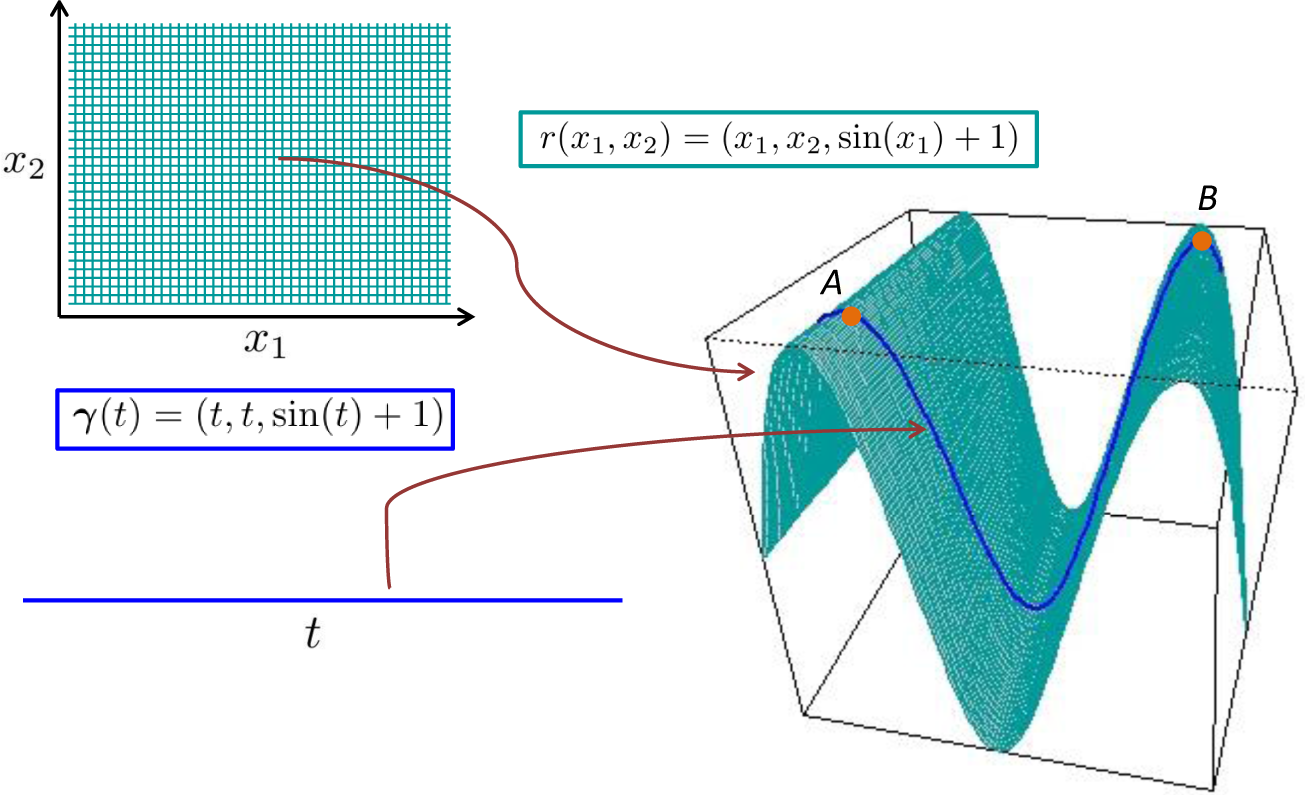
By a “diffusion on a manifold” in local coordinates, we actually mean a diffusion defined on Euclidean space. For example, a realisation of Brownian motion on the surface, S ⊂ ℝ3, defined in Figure 2 through r(x1, x2) = (x1, x2, sin(x1) + 1) will be a sample path, which is defined on S and “looks locally” like Brownian motion in a neighbourhood of any point, p ∈ S. However, the pre-image of this sample path (through r−1) will not be a realisation of a Brownian motion defined on ℝ2, owing to the nonlinearity of the mapping. Therefore, to define “Brownian motion on S”, we define some diffusion (Xt)t≥0 that takes values in ℝ2, for which the process (r(Xt))t≥0 “looks locally” like a Brownian motion (and lies on S). See [42] for more intuition here.
Our goal, therefore, is to define a diffusion on Euclidean space, which, when mapped onto a manifold through r, becomes the Langevin diffusion described in (24) by the above procedure. Such a diffusion takes the form:
where those objects marked with a tilde must be defined appropriately. The next few paragraphs are technical, and readers aiming to simply grasp the key points may wish to skip to the end of this Subsection.
We turn first to , which we use to denote Brownian motion on a manifold. Intuitively, we may think of a construction based on embedded manifolds, by setting , and for each increment sampling some random vector in the tangent space TpM, and then moving along the manifold in the prescribed direction for an infinitesimal period of time before re-sampling another velocity vector from the next tangent space [42]. In fact, we can define such a construction using Stratonovich calculus and show that the infinitesimal generator can be written using only local coordinates [28]. Here, we instead take the approach of generalising the generator directly from Euclidean space to the local coordinates of a manifold, arriving at the same result. We then deduce the stochastic differential equation describing in Itô form using (20).
For a standard Brownian motion on , where Δ denotes the Laplace operator:
Substituting into (20) trivially gives bi(x) = 0 ∀i, Vij(x) = 1{i=j}, as required. The Laplacian, Δf(x), is the divergence of the gradient vector field of some function, f ∈ C2(ℝn), and its value at x ∈ ℝn can be thought of as the average value of f in some neighbourhood of x [43].
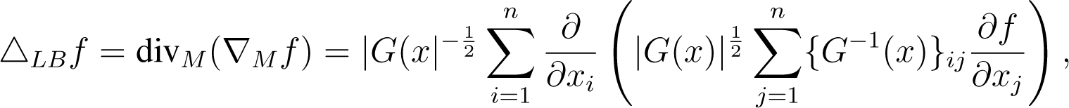
To define a Brownian motion on any manifold, the gradient and divergence must be generalised. We provide a full derivation in Appendix B, which shows that the gradient operator on a manifold can be written in local coordinates as ∇M = G−1(x)∇. Combining with the operator, divM, we can define a generalisation of the Laplace operator, known as the Laplace–Beltrami operator (e.g., [44,45]), as:

for some .
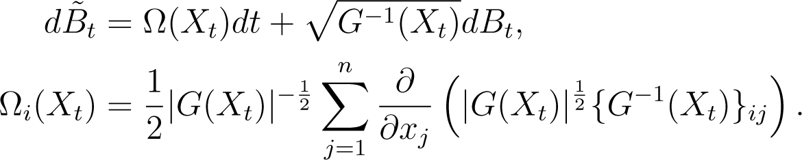
The generator of a Brownian motion on M is ΔLB/2 [44]. Using (20), the resulting diffusion has dynamics given by:

Those familiar with the Itô formula will not be surprised by the additional drift term, Ω(Xt). As Itô integrals do not follow the chain rule of ordinary calculus, non-linear mappings of martingales, such as (Bt)t≥0, typically result in drift terms being added to the dynamics (e.g., [27]).
To define , we simply note that this is again the gradient operator on a general manifold, so . For the density, , we note that this density will now implicitly be defined with respect to the volume measure, , on the manifold. Therefore, to ensure the diffusion (39) has the correct invariant density with respect to the Lebesgue measure, we define:
Putting these three elements together, Equation (39) becomes:
which, upon simplification, becomes:
It can be shown that this diffusion has invariant Lebesgue density π(x), as required [33]. Intuitively, when a set is mapped onto the manifold, distances are changed by a factor, . Therefore, to end up with the initial distances, they must first be changed by a factor of before the mapping, which explains the volatility term in Equation (43).
The resulting Metropolis–Hastings proposal kernel for this “MALA on a manifold” was clarified in [33] and is given by:
where λ2 is a tuning parameter. The nonlinear drift term here is slightly different to that reported in [1,32], for reasons discussed in [33].
4.4. Choosing a Metric
We now turn to the question of which metric structure to put on the manifold, or equivalently, how to choose G(x). In this section, we sometimes switch notation slightly, denoting the target density, π(x|y), as some of the discussion is directed towards Bayesian inference, where π(·) is the posterior distribution for some parameter, x, after observing some data, y. The problem statement is: what is an appropriate choice of distance between points in the sample space of a given probability distribution?
A related (but distinct) question is how to define a distance between two probability distributions from the same parametric family, but with different parameters. This has been a key theme in information geometry, explored by Rao [46] and others [2] for many years. Although generic measures of distance between distributions (such as total variation) are often appropriate, based on information-theoretic principles, one can deduce that for a given parametric family, , it is in some sense natural to consider this “space of distributions” to be a manifold, where the Fisher information is the matrix, G(x) (with the α = 0 connection employed; see [2] for details).
Because of this, Girolami and Calderhead [1] proposed a variant of the Fisher metric for geometric Markov chain Monte Carlo, as:
where π(x|y) ∝ f (y|x)π0(x) is the target density, f denotes the likelihood and π0the prior. The metric is tailored to Bayesian problems, which are a common use for MCMC, so the Fisher information is combined with the negative Hessian of the log-prior. One can also view this metric as the expected negative Hessian of the log target, since this naturally reduces to (46).
The motivation for a Hessian-style metric can also be understood from studying MCMC proposals. From (45) and by the same logic as for general pre-conditioning methods [32], the objective is to choose G−1(x) to match the covariance structure of π(x|y) locally If the target density were Gaussian with covariance matrix, Σ, then:
In the non-Gaussian case, the negative Hessian is no longer constant, but we can imagine that it matches the correlation structure of π(x|y) locally at least. Such ideas have been discussed in the geostatistics literature previously [47]. One problem with simply using (47) to define a metric is that unless π(x|y) is log-concave, the negative Hessian will not be globally positive-definite, although Petra et al. [48] conjecture that it may be appropriate for use in some realistic scenarios and suggest some computationally efficient approximation procedures [48].
Example: Take π(x) ∝ 1/(1 + x2), and set G(x) = −∂2 log π(x)/∂x2. Then, G−1(x) = (1 + x2)2/(2 − 2x2), which is negative if x2 > 1, so unusable as a proposal variance.
Girolami and Calderhead [1] use the Fisher metric in part to counteract this problem. Taking expectations over the data ensures that the likelihood contribution to G(x) in (46) will be positive (semi-)definite globally (e.g., [49]); so, provided a log-concave prior is chosen, then (46) should be a suitable choice for G(x). Indeed, Girolami and Calderhead [1] provide several examples in which geometric MCMC methods using this Fisher metric perform better than their “non-geometric” counterparts.
Betancourt [50] also starts from the viewpoint that the Hessian (47) is an appropriate choice for G(x) and defines a mapping from the set of n × n matrices to the set of positive-definite n × n matrices by taking a “smooth” absolute value of the eigenvalues of the Hessian. This is done in a way such that derivatives of G(x) are still computable, inspiring the author to the name, SoftAbs metric. For a fixed value of x, the negative Hessian, H(x), is first computed and, then, decomposed into UTDU, where D is the diagonal matrix of eigenvalues. Each diagonal element of D is then altered by the mapping tα: ℝ → ℝ, given by:
where α is a tuning parameter (typically chosen to be as large as possible for which eigenvalues remain non-zero numerically). The function, tα, acts as an absolute value function, but also uplifts eigenvalues, which are close to zero to ≈ 1/α. It should be noted that while the Fisher metric is only defined for models in which a likelihood is present and for which the expectation is tractable, the SoftAbs metric can be found for any target distribution, π(·).
Many authors (e.g., [1,48]) have noted that for many problems, the terms involving derivatives of G(x) are often small, and so, it is not always worth the computational effort of evaluating them. Girolami and Calderhead [1] propose the simplified manifold, MALA, in which proposals are of the form:
Using this method means derivatives of G(x) are no longer needed, so more pragmatic ways of regularising the Hessian are possible. One simple approach would be to take the absolute values of each eigenvalue, giving G(x) = UT|D|U, where H(x) = UTDU is the negative Hessian and |D| is a diagonal matrix with {|D|}ii = |λi| (this approach may fall into difficulties if eigenvalues are numerically zero). Another would be choosing G(x) as the “nearest” positive-definite matrix to the negative Hessian, according to some distance metric on the set of n × n matrices. The problem has, in fact, been well-studied in mathematical finance, in the context of finding correlations using incomplete data sets [51], and tackled using distances induced by the Frobenius norm. Approximate solution algorithms are discussed in Higham [51]. It is not clear to us at present whether small changes to the Hessian would result in large changes to the corresponding positive definite matrix under a given distance or, indeed, whether given a distance metric on the space of matrices, there is always a well-defined unique “nearest” positive definite matrix. Below, we provide two simple examples, here showing how a “Hessian-style metric” can alleviate some of the difficulties associated with both heavy and light-tailed target densities.
Example: Take π(x) ∝ 1/(1 + x2), and set G(x) = | − ∂2 log π(x)/∂x2|. Then, G−1(x) ∇ log π(x) = −x(1 + x2)/| 1 − x2|, which no longer tends to zero as |x| → ∞, suggesting a manifold variant of MALA with a Hessian-style metric may avoid some of the pitfalls of the standard algorithm. Note that the drift may become very large if |x| ≈ 1, but since this event occurs with probability zero, we do not see it as a major cause for concern.
Example: Take π(x) ∝ e−x4, and set G(x) = | − ∂2 log π(x)/∂x2|. Then, G−1(x) ∇ log π(x) = −x/3, which is O(x), so alleviating the problem of spiralling proposals for light-tailed targets demonstrated by MALA in an earlier example.
Other choices for G(x) have been proposed, which are not based on the Hessian. These have the advantage that gradients need not be computed (either analytically or using computational methods). Sejdinovic et al. [52] propose a Metropolis–Hastings method, which can be viewed as a geometric variant of the RWM, where the choice for G(x) is based on mapping samples to an appropriate feature space, and performing principal component analysis on the resulting features to choose a local covariance structure for proposals.
If we consider the RWM with Gaussian proposals to be a Euler–Maruyama discretisation of Brownian motion on a manifold, then proposals will take the form . If we assume (like in the simplified manifold MALA) that Ω(x) ≈ 0, then we have proposals centred at the current point in the Markov chain with a local covariance structure (the full Hastings acceptance rate must now be used as q(x′|x) ≠ q(x|x′) in general).
As no gradient information is needed, the Sejdinovic et al. metric can be used in conjunction with the pseudo-marginal MCMC algorithm, so that π(x|y) need not be known exactly. Examples from the article demonstrate the power of the approach [52].
An important property of any Riemannian metric is how it transforms under coordinate change (e.g., [2]). The Fisher information metric commonly studied in information geometry is an example of a “coordinate invariant” choice for G(x). If we consider two parametrisations for a statistical model given by x and z = t(x), computing the Fisher information under x and then transforming this matrix using the Jacobian for the mapping, t, will give the same result as computing the Fisher information under z. It should be noted that because of either the prior contribution in (46) or the nonlinear transformations applied in other cases, none of the metrics we have reviewed here have this property, which means that we have no principled way of understanding how G(x) will relate to G(z). It is intuitive, however, that using information from all of π(x), rather than only the likelihood contribution, f(y|x), would seem sensible when trying to sample from π(·).
5. Survey of Applications
Rather than conduct our own simulation study, we instead highlight some cases in the literature where geometric MCMC methods have been used with success.
Martin et al. [53] consider Bayesian inference for a statistical inverse problem, in which a surface explosion causes seismic waves to travel down into the ground (the subsurface medium). Often, the properties of the subsurface vary with distance from ground level or because of obstacles in the medium, in which case, a fraction of the waves will scatter off these boundaries and be reflected back up to ground level at later times. The observations here are the initial explosion and the waves, which return to the surface, together with return times. The challenge is to infer the properties of the subsurface medium from this data. The authors construct a likelihood based on the wave equation for the data and perform Bayesian inference using a variant of the manifold MALA. Figures are provided showing the local correlations present in the posterior and, therefore, highlighting the need for an algorithm that can navigate the high density region efficiently. Several methods are compared in the paper, but the variant of MALA that incorporates a local correlation structure is shown to be the most efficient, particularly as the dimension of the problem increases [53].
Calderhead and Girolami [54] dealt with two models for biological phenomena based on nonlinear dynamical systems. A model of circadian control in the Arabidopsis thaliana plant comprised a system of six nonlinear differential equations, with twenty two parameters to be inferred. Another model for cell signalling consisted of a system of six nonlinear differential equations with eight parameters, with inference complicated by the fact that observations of the model are not recorded directly [54]. The resulting inference was performed using RWM, MALA and geometric methods, with the results highlighting the benefits of taking the latter approach. The simplified variant of MALA on a manifold is reported to have produced the most efficient inferences overall, in terms of effective sample size per unit of computational time.
Stathopoulos and Girolami [55] considered the problem of inferring parameters in Markov jump processes. In the paper, a linear noise approximation is shown, which can make inference in such models more straightforward, enabling an approximate likelihood to be computed. Models based on chemical reaction dynamics are considered; one such from chemical kinetics contained four unknown parameters; another from gene expression consisted of seven. Inference was performed using the RWM, the simplified manifold MALA and Hamiltonian methods, with the MALA reported as most efficient according to the chosen diagnostics. The authors note that the simplified manifold method is both conceptually simple and able to account for local correlations, making it an attractive choice for inference [55].
Konukoglu et al. [56] designed a method for personalising a generic model for a physiological process to a specific patient, using clinical data. The personalisation took the form of patient-specific parameter inference. The authors highlight some of the difficulties of this task in general, including the complexity of the models and the relative sparsity of the datasets, which often result in a parameter identifiability issue [56]. The example discussed in the paper is the Eikonal-diffusion model describing electrical activity in cardiac tissue, which results in a likelihood for the data based on a nonlinear partial differential equation, combined with observation noise [56]. A method for inference was developed by first approximating the likelihood using a spectral representation and then using geometric MCMC methods on the resulting approximate posterior. The method was first evaluated on synthetic data and then repeated on clinical data taken from a study for ventricular tachycardia radio-frequency ablation [56].
6. Discussion
The geometric viewpoint in not necessary to understand manifold variants of the MALA. Indeed, several authors [32,33] have discussed these algorithms without considering them to be “geometric”, rather simply Metropolis–Hastings methods in which proposal kernels have a position-dependent covariance structure. We do not claim that the geometric view is the only one that should be taken. Our goal is merely to point out that such position-dependent methods can often be viewed as methods defined on a manifold and that studying the structure of the manifold itself may lead to new insights on the methods. For example, taking the geometric viewpoint and noting the connection with information geometry enabled Girolami and Calderhead to adopt the Fisher metric for calculations [1]. We list here a few open questions on which the geometric viewpoint may help shed some insight.
Computationally-minded readers will have noted that using position-dependent covariance matrices adds a significant computational overhead in practice, with additional O(n3) matrix inversions required at each step of the corresponding Metropolis–Hastings algorithms. Clearly, there will be many problems for which the matrix, G(x), does not change very much, and therefore, choosing a constant covariance G−1(x) = Σ may result in a more efficient algorithm overall. Geometrically, this would correspond to a manifold with scalar curvature close to zero everywhere. It may be that geometric ideas could be used to understand whether the manifold is flat enough that a constant choice of G(x) is sufficient. To make sense of this truly would require a relationship between curvature, an inherently local property and more global statements about the manifold. Many results in differential geometry, beginning with the celebrated Gauss–Bonnet theorem, have previously related global and local properties in this way [57]. It is unknown to the authors whether results exist relating the curvature of a manifold to some global property, but this is an interesting avenue for further research.
A related question is when to choose the simplified manifold MALA over the full method. Problems in which the term, ‖Λ(x)‖, is sufficient large to warrant calculation correspond to those for which the manifold has very high curvature in many places; so again, making some global statement related to curvature could help here.
Although there is a reasonably intuitive argument for why the Hessian is an appropriate starting point for G(x), the lack of positive-definiteness may be seen as a cause for concern by some. After all, it could be argued that if the curvature is not positive-definite in a region, then how can it be a reasonable approximation to the local covariance structure. Many statistical models used to describe natural phenomena are characterised by distributions with heavy tails or multiple modes, for which this is the case. In addition, for target densities of the form π(x) ∝ e−|x|, the Hessian is everywhere equal to zero!The attempts to force positive-definiteness we have described will typically result in small moves being proposed in such regions of the sample space, which may not be an optimal strategy. Much work in information geometry has centred on the geometry of Hessian structures [58], and some insights from this field may help to better understand the question of choosing an appropriate metric. In addition, the field of pseudo-Riemannian geometry deals with forms of G(x), which need not be positive-definite [39]; so again, understanding could be gained from here.
Some recent work in high-dimensional inference has centred on defining MCMC methods for which efficiency scales O(1) with respect to the dimension, n, of π(·) [19,59]. In the case where X takes values in some infinite-dimensional function space, this can be done provided a Gaussian prior measure is defined for X. A striking result from infinite-dimensional probability spaces is that two different probability measures defined over some infinite dimensional space have a striking tendency to have disjoint supports [60]. The key challenge for MCMC is to define transition kernels for which proposed moves are inside the support for π(·). A straight-forward approach is to define proposals for which the prior is invariant, since the likelihood contribution to the posterior typically will not alter its support from that of the prior [19]. However, the posterior may still look very different from the prior, as noted in [61], so this proposal mechanism, though O(1), can still result in slow exploration. Understanding the geometry of the support and defining methods that incorporate the likelihood term, but also respect this geometry, so as to ensure proposals remain in support of π(·), is an intriguing research proposition.
The methods reviewed in this paper are based on first order Langevin diffusions. Algorithms have also been developed that are based on second order Langevin diffusions, in which a stochastic differential equation governs the behaviour of the velocity of a process [62,63]. A natural extension to the work of Girolami and Calderhead [1] and Xifara et al. [33] would be to map such diffusions onto a manifold and derive Metropolis–Hastings proposal kernels based on the resulting dynamics. The resulting scheme would be a generalisation of [63], though the most appropriate discretisation scheme for a second order process to facilitate sampling is unclear and perhaps a question worthy of further exploration.
We have focused primarily here on the sample space and on defining an appropriate manifold on which to construct Markov chains. In some inference problems, however, the sample space is a pre-defined manifold, for example the set of n × n rotation matrices, commonly found in the field of directional statistics [64]. Such manifolds are often not globally mappable to Euclidean n-space. Methods have been devised for sampling from such spaces [65,66]. In order to use the methods described here for such problems, an appropriate approach for switching between coordinate patches at the relevant time would need to be devised, which could be an interesting area of further study.
Alongside these geometric problems, we can also discuss geometric MCMC methods from a statistical perspective. The last example given in the previous section hinted that the manifold MALA may cope better with target distributions with heavy tails. In fact, Latuszynski et al. [67] have shown that, in one dimension, the manifold MALA is geometrically ergodic for a class of targets of the form π(x) ∝ exp(− |x|β) for any choice of β ≠ 1. This incorporates cases where tails are heavier than exponential and lighter than Gaussian, two scenarios under which geometric ergodicity fails for the MALA.
Finding optimal acceptance rates and scaling of λ with dimension are two other related challenges. In this case, the picture is more complex. Traditional results have been shown for Metropolis–Hastings methods in the case where target distributions are independent and identically-distributed or some other suitable symmetry and regularity in the shape of π(·). Manifold methods are, however, specifically tailored to scenarios in which this is not the case, scenarios in which there is a high correlation between components of x, which changes depending on the value of x. It is less clear how to proceed with finding relevant results that can serve as guidelines to practitioners here. Indeed, Sherlock [18] notes that a requirement for optimal acceptance rate results for the RWM to be appropriate is that the curvature of π(x) does not change too much, yet this is the very scenario in which we would want to use a manifold method.
Acknowledgments
We thank the two reviewers for helpful comments and suggestions. Samuel Livingstone is funded by a PhD Scholarship from Xerox Research Centre Europe. Mark Girolami is funded by an Engineering and Physical Sciences Research Council Established Career Research Fellowship, EP/J016934/1, and a Royal Society Wolfson Research Merit Award.
Author Contributions
The article was written by Samuel Livingstone under the guidance of Mark Girolami. All authors have read and approved the final manuscript.
Conflicts of Interest
The authors declare no conflict of interest.
Appendix
A. Total Variation Distance
We show how to obtain (10) from (9). Denoting two probability distributions, μ(·) and ν(·), and associated densities, μ(x) and ν(x), we have:
Define the set . To see that , note that , and the result follows from properties of (e.g., [68]). Now, for any :
and similarly:
so, the supremum will be attained either at B or Bc. However, since μ( ) = ν( ) = 1, then:
so that
Using these facts gives an alternative characterisation of the total variation distance as:

as required.
B. Gradient and Divergence Operators on a Riemannian Manifold
The gradient of a function on ℝn is the unique vector field, such that, for any unit vector, u:
the directional derivative of f along u at x ∈ ℝn.
On a manifold, the gradient operator, ∇M, can still be defined, such that the inner product gp(∇M f(x),u)=Du[f(x)]. Setting ∇M = G(x)−1∇ gives:
which is equal to the directional derivative along u as required.
The divergence of some vector field, υ, at a point, x ∈ ℝn, is the net outward flow generated by υ through some small neighbourhood of x. Mathematically, the divergence of υ(x) ∈ ℝ3 is given by ∑i ∂υi/∂xi. On a more general manifold, the divergence is also a sum of derivatives, but here, they are covariant derivatives. A short introduction is provided in Appendix C. Here, we simply state that the covariant derivative of a vector field, υ, at a point p ∈ M is the orthogonal projection of the directional derivative onto the tangent space, TpM. Intuitively, a vector field on a manifold is a field of vectors, each of which lie in the tangent space to a point, p ∈ M. It only makes sense therefore to discuss how vector fields change along the manifold or in the direction of vectors, which also lie in the tangent space. Although the idea seems simple, the covariant derivative has some attractive geometric properties; notably, it can be completely written in local coordinates,and, so, does not depend on knowledge of an embedding in some ambient space.
The divergence of a vector field, υ, defined on a manifold, M, at the point, p ∈ M, is defined as:
where ei denotes the i-th basis vector for the tangent space, TpM, at p ∈ M, and υi denotes the i-th coefficient. This can be written in local coordinates (see Appendix C) as:
and can be combined with ∇M to form the Laplace–Beltrami operator (41).
C. Vector Fields and the Covariant Derivative
Here, we provide a short introduction to vector fields and differentiation on a smooth manifold; see [38,39]. The following geometric notation is used here: (i) vector components are indexed with a superscript, e.g., υ = (υ1, …,υn); and (ii) repeated subscripts and superscripts are summed over, e.g., υiei = ∑iυiei (known as the Einstein summation convention).
For any smooth manifold, M, the set of all tangent vectors to points on M is known as the tangent bundle and denoted TM.
A Cr vector field defined on M is a mapping that assigns to each point, p ∈ M, a tangent vector, υ(p) ∈ TpM. In addition, the components of υ(p) in any basis for TpM must also be Cr [38]. We will denote the set of all vector fields on M as Γ(TM). For some vector field, υ ∈ Γ(TM), at any point, p ∈ M, the vector, υ(p) ∈ TpM, can be written as a linear combination of some n basis vectors {e1,…, en} as υ = υiei. To understand how υ will change in a particular direction along M, it only makes sense, therefore, to consider derivatives along vectors in TpM. Two other things must be considered when defining a derivative along a manifold: (i) how the components, υi, of each basis vector will change; and (ii) how each basis vector, ei, itself will change. For the usual directional derivative on ℝn, the basis vectors do not change, as the tangent space is the same at each point, but for a more general manifold, this is no longer the case: the ei’s are referred to as a “local” basis for each TpM.
The covariant derivative, Dc, is defined so as to account for these shortcomings. When considering differentiation along a vector, u* ∉ TpM, u* is simply projected onto the tangent space. The derivative with respect to any u ∈ TpM can now be decomposed into a linear combination of derivatives of basis vectors and vector components:
where the argument, p, has been dropped, but is implied for both components and local basis vectors. The operator, , is defined to be linear in both u and υ and to satisfy the product rule [38]; so, Equation (51) can be decomposed into:
The operator, Dc, need, therefore, only be defined along the direction of basis vectors ei and for vector component υi and basis vector ei arguments.
For components υi, is defined as simply the partial derivative ∂jυi := ∂υi/∂xj. The directional derivative of some basis vector ei along some ej is best understood through the example of a regular surface Σ ⊂ ℝ3. Here, Dej[ei] will be a vector, w ∈ ℝ3. Taking the basis for this space at the point, p, as , where denotes the unit normal to TpΣ, we can write . The covariant derivative, , is simply the projection of w onto TpΣ, given by w* = αe1 + βe2. More generally, at some point, p, in a smooth manifold, M, the covariant derivative (with upper and lower indices summed over). The coefficients, , are known as the Christoffel symbols: denotes the coefficient of the k-th basis vector when taking the derivative of the i-th with respect to the j-th. If a Riemannian metric, g, is chosen for M; then, they can be expressed completely as a function of g (or in local coordinates as a function of the matrix, G). Using these definitions, Equation (52) can be re-written as:
The divergence of a vector field, υ ∈ Γ(TM), at the point, p ∈ M, is given by:
where, again, repeated indices are summed over. If M = ℝn, this reduces to the usual sum of partial derivatives, ∂iυi. On a more general manifold, M, the equivalent expression is:”’
where, again, repeated indices are summed. As has been previously stated, if a metric, g, and coordinate chart is chosen for M, the Christoffel symbols can be written in terms of the matrix, G(x). In this case [69]:
so Equation (55) becomes:
where υ = υ(x).
References
- Girolami, M.; Calderhead, B. Riemann manifold Langevin and Hamiltonian Monte Carlo methods. J. R. Stat. Soc. Ser. B 2011, 73, 123–214. [Google Scholar]
- Amari, S.I.; Nagaoka, H. Methods of Information Geometry; American Mathematical Society: Providence, RI, USA, 2007; Volume 191. [Google Scholar]
- Marriott, P.; Salmon, M. Applications of Differential Geometry to Econometrics; Cambridge University Press: Cambridge, UK, 2000. [Google Scholar]
- Betancourt, M.; Girolami, M. Hamiltonian Monte Carlo for Hierarchical Models 2013, arXiv, 1312.0906.
- Neal, R. MCMC using Hamiltonian Dynamics. In Handbook of Markov Chain Monte Carlo; Chapman and Hall/CRC: Boca Raton, FL, USA, 2011; pp. 113–162. [Google Scholar]
- Betancourt, M.; Stein, L.C. The Geometry of Hamiltonian Monte Carlo 2011, arXiv, 1112.4118.
- Robert, C.P.; Casella, G. Monte Carlo Statistical Methods; Springer: New York, NY, USA, 2004; Volume 319. [Google Scholar]
- Tierney, L. Markov chains for exploring posterior distributions. Ann. Stat 1994, 22, 1701–1728. [Google Scholar]
- Kipnis, C.; Varadhan, S. Central limit theorem for additive functionals of reversible Markov processes and applications to simple exclusions. Commun. Math. Phys 1986, 104, 1–19. [Google Scholar]
- R Core Team, R: A Language and Environment for Statistical Computing; R Foundation for Statistical Computing: Vienna, Austria, 2012.
- Plummer, M.; Best, N.; Cowles, K.; Vines, K. CODA: Convergence diagnosis and output analysis for MCMC. R. News 2006, 6, 7–11. [Google Scholar]
- Gibbs, A.L.; Su, F.E. On choosing and bounding probability metrics. Int. Stat. Rev 2002, 70, 419–435. [Google Scholar]
- Jones, G.L.; Hobert, J.P. Honest exploration of intractable probability distributions via Markov chain Monte Carlo. Stat. Sci 2001, 16, 312–334. [Google Scholar]
- Jones, G.L. On the Markov chain central limit theorem. Probab. Surv 2004, 1, 299–320. [Google Scholar]
- Gelman, A.; Rubin, D.B. Inference from iterative simulation using multiple sequences. Stat. Sci 1992, 7, 457–472. [Google Scholar]
- Sherlock, C.; Fearnhead, P.; Roberts, G.O. The random walk Metropolis: Linking theory and practice through a case study. Stat. Sci 2010, 25, 172–190. [Google Scholar]
- Sherlock, C.; Roberts, G. Optimal scaling of the random walk Metropolis on elliptically symmetric unimodal targets. Bernoulli 2009, 15, 774–798. [Google Scholar]
- Sherlock, C. Optimal scaling of the random walk Metropolis: General criteria for the 0.234 acceptance rule. J. Appl. Probab 2013, 50, 1–15. [Google Scholar]
- Beskos, A.; Kalogeropoulos, K.; Pazos, E. Advanced MCMC methods for sampling on diffusion pathspace. Stoch. Processes Appl 2013, 123, 1415–1453. [Google Scholar]
- Roberts, G.O.; Rosenthal, J.S. Optimal scaling for various Metropolis–Hastings algorithms. Stat. Sci 2001, 16, 351–367. [Google Scholar]
- Roberts, G.O.; Tweedie, R.L. Geometric convergence and central limit theorems for multidimensional Hastings and Metropolis algorithms. Biometrika 1996, 83, 95–110. [Google Scholar]
- Mengersen, K.L.; Tweedie, R.L. Rates of convergence of the Hastings and Metropolis algorithms. Ann. Stat 1996, 24, 101–121. [Google Scholar]
- Jarner, S.F.; Hansen, E. Geometric ergodicity of Metropolis algorithms. Stoch. Processes Appl 2000, 85, 341–361. [Google Scholar]
- Christensen, O.F.; Møller, J.; Waagepetersen, R.P. Geometric ergodicity of Metropolis–Hastings algorithms for conditional simulation in generalized linear mixed models. Methodol. Comput. Appl. Probab 2001, 3, 309–327. [Google Scholar]
- Neal, P.; Roberts, G. Optimal scaling for random walk Metropolis on spherically constrained target densities. Methodol. Comput. Appl. Probab 2008, 10, 277–297. [Google Scholar]
- Jarner, S.F.; Tweedie, R.L. Necessary conditions for geometric and polynomial ergodicity of random-walk-type. Bernoulli 2003, 9, 559–578. [Google Scholar]
- Øksendal, B. Stochastic Differential Equations; Springer: New York, NY, USA, 2003. [Google Scholar]
- Rogers, L.C.G.; Williams, D. Diffusions, Markov Processes and Martingales: Volume 2, Itô Calculus; Cambridge University Press: Cambridge, UK, 2000; Volume 2. [Google Scholar]
- Meyn, S.P.; Tweedie, R.L. Stability of Markovian processes III: Foster–Lyapunov criteria for continuous-time processes. Adv. Appl. Probab 1993, 25, 518–518. [Google Scholar]
- Coffey, W.; Kalmykov, Y.P.; Waldron, J.T. The Langevin Equation: with Applications to Stochastic Problems in Physics, Chemistry, and Electrical Engineering; World Scientific: Singapore, Singapore, 2004; Volume 14. [Google Scholar]
- Roberts, G.O.; Tweedie, R.L. Exponential convergence of Langevin distributions and their discrete approximations. Bernoulli 1996, 2, 341–363. [Google Scholar]
- Roberts, G.O.; Stramer, O. Langevin diffusions and Metropolis–Hastings algorithms. Methodol. Comput. Appl. Probab 2002, 4, 337–357. [Google Scholar]
- Xifara, T.; Sherlock, C.; Livingstone, S.; Byrne, S.; Girolami, M. Langevin diffusions and the Metropolis-adjusted Langevin algorithm. Stat. Probab. Lett 2013, 91, 14–19. [Google Scholar]
- Jeffreys, H. An invariant form for the prior probability in estimation problems. Proc. R. Soc. Lond. Ser. A Math. Phys. Sci 1946, 186, 453–461. [Google Scholar]
- Critchley, F.; Marriott, P.; Salmon, M. Preferred point geometry and statistical manifolds. Ann. Stat 1993, 21, 1197–1224. [Google Scholar]
- Marriott, P. On the local geometry of mixture models. Biometrika 2002, 89, 77–93. [Google Scholar]
- Barndorff-Nielsen, O.; Cox, D.; Reid, N. The role of differential geometry in statistical theory. Int. Stat. Rev 1986, 54, 83–96. [Google Scholar]
- Boothby, W.M. An Introduction to Differentiable Manifolds and Riemannian Geometry; Academic Press: San Diego, CA, USA, 1986; Volume 120. [Google Scholar]
- Lee, J.M. Smooth Manifolds; Springer: New York, NY, USA, 2003. [Google Scholar]
- Do Carmo, M.P. Riemannian Geometry; Springer: New York, NY, USA, 1992. [Google Scholar]
- Nash, J.F., Jr. The imbedding problem for Riemannian manifolds. In The Essential John Nash; Princeton University Press: Princeton, NJ, USA, 2002; p. 151. [Google Scholar]
- Manton, J.H. A Primer on Stochastic Differential Geometry for Signal Processing 2013, arXiv, 1302.0430.
- Stewart, J. Multivariable Calculus; Cengage Learning: Boston, MA, USA, 2011. [Google Scholar]
- Hsu, E.P. Stochastic Analysis on Manifolds; American Mathematical Society: Providence, RI, USA, 2002; Volume 38. [Google Scholar]
- Kent, J. Time-reversible diffusions. Adv. Appl. Probab 1978, 10, 819–835. [Google Scholar]
- Radhakrishna Rao, C. Information and accuracy attainable in the estimation of statistical parameters. Bull. Calcutta Math. Soc 1945, 37, 81–91. [Google Scholar]
- Christensen, O.F.; Roberts, G.O.; Sköld, M. Robust Markov chain Monte Carlo methods for spatial generalized linear mixed models. J. Comput. Graph. Stat 2006, 15, 1–17. [Google Scholar]
- Petra, N.; Martin, J.; Stadler, G.; Ghattas, O. A computational framework for infinite-dimensional Bayesian inverse problems: Part II. Stochastic Newton MCMC with application to ice sheet flow inverse problems 2013, arXiv, 1308.6221. [Google Scholar]
- Pawitan, Y. In All Likelihood: Statistical Modelling and Inference Using Likelihood; Oxford University Press: Oxford, UK, 2001. [Google Scholar]
- Betancourt, M. A General Metric for Riemannian Manifold Hamiltonian Monte Carlo. In Geometric Science of Information; Springer: New York, NY, USA, 2013; pp. 327–334. [Google Scholar]
- Higham, N.J. Computing the nearest correlation matrix—a problem from finance. IMA J. Numer. Anal 2002, 22, 329–343. [Google Scholar]
- Sejdinovic, D.; Garcia, M.L.; Strathmann, H.; Andrieu, C.; Gretton, A. Kernel Adaptive Metropolis–Hastings 2013, arXiv, 1307.5302.
- Martin, J.; Wilcox, L.C.; Burstedde, C.; Ghattas, O. A stochastic Newton MCMC method for large-scale statistical inverse problems with application to seismic inversion. SIAM J. Sci. Comput 2012, 34, A1460–A1487. [Google Scholar]
- Calderhead, B.; Girolami, M. Statistical analysis of nonlinear dynamical systems using differential geometric sampling methods. Interface Focus 2011, 1, 821–835. [Google Scholar]
- Stathopoulos, V.; Girolami, M.A. Markov chain Monte Carlo inference for Markov jump processes via the linear noise approximation. Philos. Trans. R. Soc. A 2013, 371, 20110541. [Google Scholar]
- Konukoglu, E.; Relan, J.; Cilingir, U.; Menze, B.H.; Chinchapatnam, P.; Jadidi, A.; Cochet, H.; Hocini, M.; Delingette, H.; Jaïs, P.; et al. Efficient probabilistic model personalization integrating uncertainty on data and parameters: Application to eikonal-diffusion models in cardiac electrophysiology. Prog. Biophys. Mol. Biol 2011, 107, 134–146. [Google Scholar]
- Do Carmo, M.P.; Do Carmo, M.P. Differential Geometry of Curves and Surfaces; Englewood Cliffs: Prentice-Hall, NJ, USA, 1976; Volume 2. [Google Scholar]
- Shima, H. The Geometry of Hessian Structures; World Scientific: Singapore, Singapore, 2007; Volume 1. [Google Scholar]
- Cotter, S.; Roberts, G.; Stuart, A.; White, D. MCMC methods for functions: Modifying old algorithms to make them faster. Stat. Sci 2013, 28, 424–446. [Google Scholar]
- Da Prato, G.; Zabczyk, J. Stochastic Equations in Infinite Dimensions; Cambridge University Press: Cambridge, UK, 2008. [Google Scholar]
- Law, K.J. Proposals which speed up function-space MCMC. J. Comput. Appl. Math 2014, 262, 127–138. [Google Scholar]
- Ottobre, M.; Pillai, N.S.; Pinski, F.J.; Stuart, A.M. A Function Space HMC Algorithm With Second Order Langevin Diffusion Limit 2013, arXiv, 1308.0543.
- Horowitz, A.M. A generalized guided Monte Carlo algorithm. Phys. Lett. B 1991, 268, 247–252. [Google Scholar]
- Mardia, K.V.; Jupp, P.E. Directional Statistics; Wiley: New York, NY, USA, 2009; Volume 494. [Google Scholar]
- Byrne, S.; Girolami, M. Geodesic Monte Carlo on embedded manifolds. Scand. J. Stat 2013, 40, 825–845. [Google Scholar]
- Diaconis, P.; Holmes, S.; Shahshahani, M. Sampling from a manifold. In Advances in Modern Statistical Theory and Applications: A Festschrift in Honor of Morris L. Eaton; Institute of Mathematical Statistics: Washington, DC, USA, 2013; pp. 102–125. [Google Scholar]
- Latuszynski, K.; Roberts, G.O.; Thiery, A.; Wolny, K. Discussion on “Riemann manifold Langevin and Hamiltonian Monte Carlo methods” (by Girolami, M. and Calderhead, B.). J. R. Stat. Soc. Ser. B 2011, 73, 188–189. [Google Scholar]
- Capinski, M.; Kopp, P.E. Measure, Integral and Probability; Springer: New York, NY, USA, 2004. [Google Scholar]
- Schutz, B.F. Geometrical Methods of Mathematical Physics; Cambridge University Press: Cambridge, UK, 1984. [Google Scholar]


© 2014 by the authors; licensee MDPI, Basel, Switzerland This article is an open access article distributed under the terms and conditions of the Creative Commons Attribution license (http://creativecommons.org/licenses/by/3.0/).
Share and Cite
Livingstone, S.; Girolami, M. Information-Geometric Markov Chain Monte Carlo Methods Using Diffusions. Entropy 2014, 16, 3074-3102. https://doi.org/10.3390/e16063074
Livingstone S, Girolami M. Information-Geometric Markov Chain Monte Carlo Methods Using Diffusions. Entropy. 2014; 16(6):3074-3102. https://doi.org/10.3390/e16063074
Chicago/Turabian StyleLivingstone, Samuel, and Mark Girolami. 2014. "Information-Geometric Markov Chain Monte Carlo Methods Using Diffusions" Entropy 16, no. 6: 3074-3102. https://doi.org/10.3390/e16063074