On the Fisher Metric of Conditional Probability Polytopes

Abstract

We consider three different approaches to define natural Riemannian metrics on polytopes of stochastic matrices. First, we define a natural class of stochastic maps between these polytopes and give a metric characterization of Chentsov type in terms of invariance with respect to these maps. Second, we consider the Fisher metric defined on arbitrary polytopes through their embeddings as exponential families in the probability simplex. We show that these metrics can also be characterized by an invariance principle with respect to morphisms of exponential families. Third, we consider the Fisher metric resulting from embedding the polytope of stochastic matrices in a simplex of joint distributions by specifying a marginal distribution. All three approaches result in slight variations of products of Fisher metrics. This is consistent with the nature of polytopes of stochastic matrices, which are Cartesian products of probability simplices. The first approach yields a scaled product of Fisher metrics; the second, a product of Fisher metrics; and the third, a product of Fisher metrics scaled by the marginal distribution.

1. Introduction

The Riemannian structure of a function’s domain has a crucial impact on the performance of gradient optimization methods, especially in the presence of plateaus and local maxima. The natural gradient [1] gives the steepest increase direction of functions on a Riemannian space. For example, artificial neural networks can often be trained by following some function’s gradient on a space of probabilities. In this context, it has been observed that following the natural gradient with respect to the Fisher information metric, instead of the Euclidean metric, can significantly alleviate the plateau problem [1,2]. The Fisher information metric, which is also called Shahshahani metric [3] in biological contexts, is broadly recognized as the natural metric of probability spaces. An important argument was given by Chentsov [4], who showed that the Fisher information metric is the only metric on probability spaces for which certain natural statistical embeddings, called Markov morphisms, are isometries. More generally, Chentsov’s theorem characterizes the Fisher metric and α-connections of statistical manifolds uniquely (up to a multiplicative constant) by requiring invariance with respect to Markov morphisms. Campbell [5] gave another proof that characterizes invariant metrics on the set of non-normalized positive measures, which restrict to the Fisher metric in the case of probability measures (up to a multiplicative constant). In this paper, we explore ways of defining distinguished Riemannian metrics on spaces of stochastic matrices.

In learning theory, when modeling the policy of a system, it is often preferred to consider stochastic matrices instead of joint probability distributions. For example, in robotics applications, policies are optimized over a parametric set of stochastic matrices by following the gradient of a reward function [6,7]. The set of stochastic matrices can be parametrized in many ways, e.g., in terms of feedforward neural networks, Boltzmann machines [8] or projections of exponential families [9]. The information geometry of policy models plays an important role in these applications and has been studied by Kakade [2], Peters and co-workers [10–12], and Bagnell and Schneider [13], among others. A stochastic matrix is a tuple of probability distributions, and therefore, the space of stochastic matrices is a Cartesian product of probability simplices. Accordingly, in applications, usually a product metric is considered, with the usual Fisher metric on each factor. On the other hand, Lebanon [14] takes an axiomatic approach, following the ideas of Chentsov and Campbell, and characterizes a class of invariant metrics of positive matrices that restricts to the product of Fisher metrics in the case of stochastic matrices. We will consider three different approaches discussed in the following.

In the first part, we take another look at Lebanon’s approach for characterizing a distinguished metric on polytopes of stochastic matrices. However, since the maps considered by Lebanon do not map stochastic matrices to stochastic matrices, we will use different maps. We show that the product of Fisher metrics can be characterized by an invariance principle with respect to natural maps between stochastic matrices.

In the second part, we consider an approach that allows us to define Riemannian structures on arbitrary polytopes. Any polytope can be identified with an exponential family by using the coordinates of the polytope vertices as observables. The inverse of the moment map then defines an embedding of the polytope in a probability simplex. This embedding can be used to pull back geometric structures from the probability simplex to the polytope, including Riemannian metrics, affine connections, divergences, etc. This approach has been considered in [9] as a way to define low-dimensional families of conditional probability distributions. More general embeddings can be defined by identifying each exponential family with a point configuration, B, together with a weight function, ν. Given B and ν, the corresponding exponential family defines geometric structures on the set (conv B)°, which is the relative interior of the convex support of the exponential family Moreover, we can define natural morphisms between weighted point configurations as surjective maps between the point sets, which are compatible with the weight functions. As it turns out, the Fisher metric on (conv B)° can be characterized by invariance under these maps.

In the third part, we return to stochastic matrices. We study natural embeddings of conditional distributions in probability simplices as joint distributions with a fixed marginal. These embeddings define a Fisher metric equal to a weighted product of Fisher metrics. This result corresponds to the definitions commonly used in robotics applications.

All three approaches give very similar results. In all cases, the identified metric is a product metric. This is a sensible result, since the set of k × m stochastic matrices is a Cartesian product of probability simplices ${\mathrm{\Delta }}_{m-1}\times \cdots \times {\mathrm{\Delta }}_{m-1}={\mathrm{\Delta }}_{m-1}^k$, which suggests using the product metric of the Fisher metrics defined on the factor simplices, ∆_m−1. Indeed, this is the result obtained from our second approach. The first approach yields that same result with an additional scaling factor of 1/k. Only when stochastic matrices of different sizes are compared, the two approaches differ. The third approach yields a product of Fisher metrics scaled by the marginal distribution that defines the embedding.

Which metric to use depends on the concrete problem and whether a natural marginal distribution is defined and known. In Section 7, we do a case study using a reward function that is given as an expectation value over a joint distribution. In this simple example, the weighted product metric gives the best asymptotic rate of convergence, under the assumption that the weights are optimally chosen. In Section 8, we sum up our findings.

The contents of the paper is organized as follows. Section 2 contains basic definitions around the Fisher metric and concepts of differential geometry. In Section 3, we discuss the theorems of Chentsov, Campbell and Lebanon, which characterize natural geometric structures on the probability simplex, on the set of positive measures and on the cone of positive matrices, respectively. In Section 4, we study metrics on polytopes of stochastic matrices, which are invariant under natural embeddings. In Section 5, we define a Riemannian structure for polytopes, which generalizes the Fisher information metric of probability simplices and conditional models in a natural way. In Section 6, we study a class of weighted product metrics. In Section 7, we study the gradient flow with respect to an expectation value. Section 8 contains concluding remarks. In Appendix A, we investigate restrictions on the parameters of the metrics characterized in Sections 3 and 4 that make them positive definite. Appendix B contains the proofs of the results from Section 4.

2. Preliminaries

We will consider the simplex of probability distributions on [m] := {1,…, m}, m ≥ 2, which is given by ${\mathrm{\Delta }}_{m-1}:=\left\{{\left(p_i\right)}_i\in {\mathrm{ℝ}}^m:p_i\ge 0,{\displaystyle {\sum }_i{p}_i=1}\right\}$. The relative interior of ∆_m−1 consists of all strictly positive probability distributions on [m], and will be denoted ${\mathrm{\Delta }}_{m-1}^{°}$. This is a subset of ${\mathrm{ℝ}}_{+}^m$, the cone of strictly positive vectors. The set of k × m row-stochastic matrices is given by ${\mathrm{\Delta }}_{m-1}^k:=\left\{{\left(K_{ij}\right)}_{ij}\right\}\in {\mathrm{ℝ}}^{k\times m}:{\left(K_{ij}\right)}_j\in {\mathrm{\Delta }}_{m-1}$ for all i ∈ [k and is equal to the Cartesian product ×_i∈[k] ∆_m−1. The relative interior ${({\mathrm{\Delta }}_{m-1}^k)}^{\circ }$ is a subset of ${\mathrm{ℝ}}_{+}^{k\times m}$, the cone of strictly positive matrices.

Given two random variables X and Y taking values in the finite sets [k] and [m], respectively, the conditional probability distribution of Y given X is the stochastic matrix K = (P(y|x))_{x∈[k],y∈[m]} with rows (P(y|x))_y∈[m] ∈ ∆_m−1 for all x ∈ [k]. Therefore, the polytope of stochastic matrices ${\mathrm{\Delta }}_{m-1}^k$ is called a conditional polytope.

The tangent space of ${\mathrm{ℝ}}_{+}^n$ at a point $p\in {\mathrm{ℝ}}_{+}^n$, denoted by $T_p{\mathrm{ℝ}}_{+}^n$, is the real vector space spanned by the vectors ∂₁,…, ∂_n of partial derivatives with respect to the n components. The tangent space of ${\mathrm{\Delta }}_{n-1}^{\circ }$ at a point $p\in {\mathrm{\Delta }}_{n-1}^{\circ }\subset {\mathrm{ℝ}}_{+}^n$ is the subspace $T_p{\mathrm{\Delta }}_{n-1}^{\circ }\subset T_p{\mathrm{ℝ}}_{+}^n$ consisting of the vectors:

$$u={\displaystyle \sum _i{u}_i{\partial }_i\in T_p{\mathrm{ℝ}}_{+}^n\text{with}}{\displaystyle \sum _i{u}_i=0.}$$

(1)

The Fisher metric on the positive probability simplex ${\mathrm{\Delta }}_{n-1}^{\circ }$ is the Riemannian metric given by:

$$g_p^{(n)}(u,v)={\displaystyle \sum _{i=1}^n\frac{u_i{v}_i}{p_i},\text{for all }u,v\in T_p{\mathrm{\Delta }}_{n-1}^{\circ }.}$$

(2)

The same formula (2) also defines a Riemannian metric on ${\mathrm{ℝ}}_{+}^n$, which we will denote by the same symbol. This, however, is not the only way in which the Fisher metric can be extended from ${\mathrm{\Delta }}_{n-1}^{\circ }$ to ${\mathrm{ℝ}}_{+}^n$. We will discuss other extensions in the next section (see Campbell’s theorem, Theorem 3).

Consider a smoothly parametrized family of probability distributions $\mathrm{ℳ}=\left\{{\left(p\left(x;\theta \right)\right)}_{x\in \left[n\right]}:\theta \in \Omega \right\}\subseteq {\mathrm{\Delta }}_{n-1}^{\circ }$, where $\Omega \subseteq {\mathrm{ℝ}}^d$ is open. Then, g⁽ⁿ⁾ induces a Riemannian metric on $\mathrm{ℳ}$. Denote by ${\partial }_{{\theta }_i}=\frac{\partial }{\partial {\theta }_i}$ the tangent vector corresponding to the partial derivative with respect to θ_i, for all i ∈ [d]. Then, the Fisher matrix has coordinates:

(3)

Here, it is not necessary to assume that the parameters θ_i are independent. In particular, the dimension of $\mathrm{ℳ}$ may be smaller than d, in which case the matrix is not positive definite. If the map $\Omega \to \mathrm{ℳ},\theta \mapsto p\left(·;\theta \right)$ is an embedding (i.e., a smooth injective map that is a diffeomorphism onto its image), then $g_{\theta }^{\mathrm{ℳ}}$ defines a Riemannian metric on Ω, which corresponds to the pull-back of g⁽ⁿ⁾.

Consider an embedding f: ε → ε′. The pull-back of a metric g′ on ε′ through f is defined as:

$${\left(f^{*}{g}^{\prime }\right)}_p\left(u,v\right):={g^{\prime }}_{f\left(p\right)}\left(f_{*}u,f_{*}v\right),\text{for all }u,v\in T_p\epsilon ,$$

(4)

where f_* denotes the push-forward of T_pε through f, which in coordinates is given by:

$$f_{*}:T_p\epsilon \to T_p{\epsilon }^{\prime };{\displaystyle \sum _i{u}_i{\partial }_{{\theta }_i}}\mapsto {\displaystyle \sum _j{\displaystyle \sum _i{u}_i\frac{\partial f_j(p)}{\partial {\theta }_i}{\partial }_{{{\theta }^{\prime }}_j},}}$$

(5)

where ${\left\{{\partial }_{{\theta }_i}\right\}}_i$ spans T_qε and ${\left\{{\partial }_{{{\theta }^{\prime }}_j}\right\}}_j$ spans T_f(p)ε′.

An embedding f: ε → ε′ of two Riemannian manifolds (ε, g) and (ε′, g′) is an isometry iff:

$$g_p\left(u,v\right)={\left(f^{*}{g}^{\prime }\right)}_p\left(u,v\right),\text{for all }p\in \epsilon \text{ and }u,v\in T_p\epsilon ,$$

(6)

In this case, we say that the metric g is invariant with respect to f (and g′).

3. The Results of Campbell and Lebanon

One of the theoretical motivations for using the Fisher metric is provided by Chentsov’s characterization [4], which states that the Fisher metric is uniquely specified, up to a multiplicative constant, by an invariance principle under a class of stochastic maps, called Markov morphisms. Later, Campbell [5] considered the characterization problem on the space ${\mathrm{ℝ}}_{+}^n$ instead of ${\mathrm{\Delta }}_{n-1}^{\circ }$. This simplifies the computations, since ${\mathrm{ℝ}}_{+}^n$ has a more symmetric parametrization.

Definition 1. Let 2 ≤ m ≤ n. A (row) stochastic partition matrix (or just row-partition matrix) is a matrix $Q\in {\mathrm{ℝ}}^{m\times n}$ of non-negative entries, which satisfies ${\displaystyle {\sum }_{j\in A_{i^{\prime }}}{Q}_{ij}={\delta }_{i{i}^{\prime }}}$ for an m block partition {A₁,…, A_m} of [n]. The linear map defined by:

$${\mathrm{ℝ}}_{+}^m\to {\mathrm{ℝ}}_{+}^n;p\mapsto p\cdot Q$$

(7)

is called a congruent embedding by a Markov mapping of ${\mathrm{ℝ}}_{+}^m$ to ${\mathrm{ℝ}}_{+}^n$ or just a Markov map, for short.

An example of a 3 × 5 row-partition matrix is:

$$Q=\left(\begin{array}{ccccc}1/2& 0& 1/2& 0& 0\\ 0& 1/3& 0& 2/3& 0\\ 0& 0& 0& 0& 1\end{array}\right).$$

(8)

Markov maps preserve the 1-norm and restrict to embeddings ${\mathrm{\Delta }}_{m-1}^{\circ }\to {\mathrm{\Delta }}_{n-1}^{\circ }$.

Theorem 2 (Chentsov’s theorem.).

• Let g^(m) be a Riemannian metric on${\mathrm{\Delta }}_{m-1}^{\circ }$ for m ∈ {2, 3,…}. Let this sequence of metrics have the property that every congruent embedding by a Markov mapping is an isometry. Then, there is a constant C > 0 that satisfies:

  $$g_p^{\left(m\right)}\left(u,v\right)=C{\displaystyle \sum _i\frac{u_i{v}_i}{p_i}.}$$

  (9)

• Conversely, for any C > 0, the metrics given by Equation (9) define a sequence of Riemannian metrics under which every congruent embedding by a Markov mapping is an isometry.

The main result in Campbell’s work [5] is the following variant of Chentsov’s theorem.

Theorem 3 (Campbell’s theorem.).

• Let g^(m) be a Riemannian metric on${\mathrm{ℝ}}_{+}^m$ for m ∈ {2,3,…}. Let this sequence of metrics have the property that every embedding by a Markov mapping is an isometry. Then:

  $$g_p^{\left(m\right)}\left({\partial }_i,{\partial }_j\right)=A\left(\left|p\right|\right)+{\delta }_{ij}C\left(\left|p\right|\right)\frac{\left|p\right|}{p_i},$$

  (10)

  where $\left|p\right|={\displaystyle {\sum }_{i=1}^m{p}_i}$, δ_ij is the Kronecker delta, and A and C are C^∞ functions on ${\mathrm{ℝ}}_{+}$ satisfying C(α) > 0 and A(α) + C(α) > 0 for all α > 0.

• Conversely, if A and C are C^∞ functions on${\mathrm{ℝ}}^{+}$ satisfying C(α) > 0, A(α) + C(α) > 0 for all α > 0, then Equation (10) defines a sequence of Riemannian metrics under which every embedding by a Markov mapping is an isometry.

The metrics from Campbell’s theorem also define metrics on the probability simplices ${\mathrm{\Delta }}_{m-1}^{\circ }$ for m = 2,3,…. Since the tangent vectors $\upsilon ={\displaystyle {\sum }_i{\upsilon }_i{\partial }_i\in T_p{\mathrm{\Delta }}_{m-1}^{\circ }}$ satisfy ${\displaystyle {\sum }_i{\upsilon }_i=0}$, for any two vectors $u,\upsilon \in T_p{\mathrm{\Delta }}_{m-1}^{\circ }$, also ${\displaystyle {\sum }_i{\displaystyle {\sum }_{j}A{u}_i{\upsilon }_j=0}}$ for any A. In this case, the choice of A is immaterial, and the metric becomes Chentsov’s metric.

Remark 4. Observe that Chentsov’s theorem is not a direct implication of Campbell’s theorem. However, it can be deduced from it by the following arguments. Suppose that we have a family of Riemannian simplices $\left({\mathrm{\Delta }}_{m-1}^{\circ },g^{\left(m\right)}\right)$ for m ∈ {2, 3,…}, and suppose that they are isometric with respect to Markov maps. If we can extend every g^(m) to a Riemannian metric ${\tilde{g}}^{\left(m\right)}$ on ${\mathrm{ℝ}}_{+}^m$ in such a way that the resulting spaces $\left({\mathrm{ℝ}}_{+}^m,{\tilde{g}}^{\left(m\right)}\right)$ still isometric with respect to Markov maps, then Campbell’s theorem implies that g^(m) is a multiple of the Fisher metric. Such metric extensions can be defined as follows. Consider the diffeomorphism:

$${\mathrm{\Delta }}_{m-1}^{\circ }\times {\mathrm{ℝ}}_{+}\cong {\mathrm{ℝ}}_{+}^m,\left(p,r\right)\mapsto r\cdot p.$$

(11)

Any tangent vector $u\in T_{\left(p,r\right)}{\mathrm{ℝ}}_{+}^m$ can be written uniquely as u = u_p + u_r∂_r, where u_p is tangent to $r{\mathrm{\Delta }}_{m-1}^{\circ }$. Since each Markov map f preserves the one-norm | · |, its push-forward f_* maps the tangent vector ${\partial }_r\in T_{\left(p,r\right)}{\mathrm{ℝ}}_{+}^m$ to the corresponding tangent vector ${\partial }_r\in T_{f\left(p,r\right)}{\mathrm{ℝ}}_{+}^m$; that is, f_*u = f_*u_p + u_r∂_r. Therefore,

$${\tilde{g}}_{\left(p,r\right)}^{\left(m\right)}\left(u,\upsilon \right):=g_p^{\left(m\right)}\left(u_p,{\upsilon }_p\right)+u_r{\upsilon }_r$$

(12)

is a metric on ${\mathrm{ℝ}}_{+}^m$ that is invariant under f.

In what follows, we will focus on positive matrices. In order to define a natural Riemannian metric, we can use the identification ${\mathrm{ℝ}}_{+}^{k\times m}\cong {\mathrm{ℝ}}_{+}^{km}$ and apply Campbell’s theorem. This leads to metrics of the form:

$$g_M^{\left(k,m\right)}\left({\partial }_{ij},{\partial }_{kl}\right)=A\left(\left|M\right|\right)+{\delta }_{ik}{\delta }_{jl}C\left(\left|M\right|\right)/M_{ij},$$

(13)

where ${\partial }_{ij}=\frac{\partial }{\partial M_{ij}}$ and $\left|M\right|={\displaystyle {\sum }_{ij}{M}_{ij}}$. However, a disadvantage of this approach is that the action of general Markov maps on ${\mathrm{ℝ}}_{+}^{km}$ has no natural interpretation in terms of the matrix structure. Therefore, Lebanon [14] considered a special class of Markov maps defined as follows.

Definition 5. Consider a k × l row-partition matrix R and a collection of m × n row-partition matrices Q = {Q⁽¹⁾,…, Q^(k)}. The map:

$${\mathrm{ℝ}}_{+}^{k\times m}\to {\mathrm{ℝ}}_{+}^{l\times n};M\mapsto R^{\top }\left(M\otimes Q\right)$$

(14)

is called a congruent embedding by a Markov morphism of ${\mathrm{ℝ}}_{+}^{k\times m}$ to ${\mathrm{ℝ}}_{+}^{l\times n}$ in [15]. We will refer to such an embedding as a Lebanon map. Here, the row product M ⊗ Q is defined by:

$${\left(M\otimes Q\right)}_{ab}={\left(M\cdot Q^{\left(a\right)}\right)}_{ab},\text{for all }a\in \left[k\right],b\in \left[n\right];$$

(15)

that is, the a-th row of M is multiplied by the matrix Q^(a).

In a Lebanon map, each row of the input matrix M is mapped by an individual Markov mapping Q⁽ⁱ⁾, and each resulting row is copied and scaled by an entry of R. This kind of map preserves the sum of all matrix entries. Therefore, with the identification ${\mathrm{ℝ}}_{+}^{k\times m}\cong {\mathrm{ℝ}}_{+}^{km}$, each Lebanon map restricts to a map ${\mathrm{\Delta }}_{mk-1}^{\circ }\to {\mathrm{\Delta }}_{nl-1}^{\circ }$. The set ${\mathrm{\Delta }}_{mk-1}^{\circ }$ can be identified with the set of joint distributions of two random variables. Lebanon maps can be regarded as special Markov maps that incorporate the product structure present in the set of joint probability distributions of a pair of random variables. In Section 4, we will give an interpretation of these maps.

Contrary to what is stated in [15], a Lebanon map does not map $\left({\mathrm{\Delta }}_{m-1}^k\right)°$ to $\left({\mathrm{\Delta }}_{l-1}^l\right)°$, unless k = l. Therefore, later, we will provide a characterization for the metrics on $\left({\mathrm{\Delta }}_{m-1}^k\right)°$ in terms of invariance under other maps (which are not Markov nor Lebanon maps).

The main result in Lebanon’s work [15, Theorems 1 and 2] is the following.

Theorem 6 (Lebanon’s theorem.).

• For each k ≥ 1, m ≥ 2, let g^(k,m) be a Riemannian metric on${\mathrm{ℝ}}_{+}^{k\times m}$ in such a way that every Lebanon map is an isometry. Then:

  $$g_M^{\left(k,m\right)}\left({\partial }_{ab,}{\partial }_{cd}\right)=A\left(\left|M\right|\right)+{\delta }_{ac}\left(\frac{B\left(\left|M\right|\right)}{\left|M_a\right|}+{\delta }_{bd}\frac{C\left(\left|M\right|\right)}{M_{ab}}\right)$$

  (16)

  for some differentiable functions$A,B,C\in C^{\infty }\left({\mathrm{ℝ}}_{+}\right)$.

• Conversely, let$\left\{\left({\mathrm{ℝ}}_M^{k\times m},g^{\left(k,m\right)}\right)\right\}$ be a sequence of Riemannian manifolds, with metrics g^(k,m) of the form (16) for some$A,B,C\in C^{\infty }\left({\mathrm{ℝ}}_{+}\right)$. Then, every Lebanon map is an isometry.

Lebanon does not study the question under which assumptions on $A,B,C\in C^{\infty }\left({\mathrm{ℝ}}_{+}\right)$ the formula (16) does indeed define a Riemannian metric. This question has the following simple answer, which we will prove in Appendix A:

Proposition 7. The matrix (16) is positive definite if and only if C(|M|) > 0, B(|M|) + C(|M|) > 0 and A(|M|) + B(|M|) + C(|M|) > 0.

The class of metrics (16) is larger than the class of metrics (13) derived in Campbell’s theorem. The reason is that Campbell’s metrics are invariant with respect to a larger class of embeddings.

The special case with A(|M|) = 0, B(|M|) = 0 and C(|M|) = 1 is called product Fisher metric,

$$g_M^{\left(k,m\right)}\left({\partial }_{ab},{\partial }_{cd}\right)={\delta }_{ac}{\delta }_{bd}\frac{1}{M_{ab}}.$$

(17)

Furthermore, if we restrict to $\left({\mathrm{\Delta }}_{m-1}^k\right)°$, the functions A and B do not play any role. In this case |M| = k, and we obtain the scaled product Fisher metric:

$$g_M^{\left(k,m\right)}\left({\partial }_{ab},{\partial }_{cd}\right)={\delta }_{ac}{\delta }_{bd}\frac{C\left(k\right)}{M_{ab}},$$

(18)

where $C\left(k\right):\mathbb{N}\to {\mathrm{ℝ}}_{+}$ is a positive function. As mentioned before, Lebanon’s theorem does not give a characterization of invariant metrics of stochastic matrices, since Lebanon maps do not preserve the stochasticity of the matrices. However, Lebanon maps are natural maps on the set ${\mathrm{\Delta }}_{mk-1}^{\circ }$ of positive joint distributions. In the same way as Chentsov’s theorem can be derived from Campbell’s theorem (see Remark 4), we obtain the following corollary:

Corollary 8.

• Let$\left\{\left({\mathrm{\Delta }}_{km-1}^{\circ },g^{\left(k,m\right)}\right):k\ge 1,m\ge 2\right\}$ be a double sequence of Riemannian manifolds with the property that every Lebanon map is an isometry. Then:

  $$g_P^{\left(k,m\right)}\left(u,\upsilon \right)=B{\displaystyle \sum _a{\displaystyle \sum _{b,c}\frac{u_{ab}{u}_{ac}}{\left|P_a\right|}}}+C{\displaystyle \sum _a{\displaystyle \sum _b\frac{u_{ab}{u}_{ac}}{P_{ab}},foreach}P\in {\mathrm{\Delta }}_{km-1}^{\circ },}$$

  (19)

  for some constants$B,C\in \mathrm{ℝ}$ with C > 0 and B + C > 0, where$\left|P_a\right|={\displaystyle {\sum }_b{P}_{ab}}$.

• Conversely, let$\left\{\left({\mathrm{\Delta }}_{km-1}^{\circ },g^{\left(k,m\right)}\right)\right\}$ be a sequence of Riemannian manifolds with metrics g^(k,m) of the form of Equation (19) for some$B,C\in \mathrm{ℝ}$ Then, every Lebanon map is an isometry.

Observe that these metrics agree with (a multiple of) the Fisher metric only if B = 0. The case B = 0 can also be characterized; note that Lebanon maps do not treat the two random variables symmetrically Switching the two random variables corresponds to transposing the joint distribution matrix P. When exchanging the role of the two random variables, the Lebanon map becomes P ⟼ (P^⊤ ⊗ Q)^⊤ R. We call such a map a dual Lebanon map. If we require invariance under both Lebanon maps and their duals in Theorem 6 or Corollary 8, the statements remain true with the additional restriction that B = 0 (as a function or constant, respectively).

4. Invariance Metric Characterizations for Conditional Polytopes

According to Chentsov’s theorem (Theorem 2), a natural metric on the probability simplex can be characterized by requiring the isometry of natural embeddings. Lebanon follows this axiomatic approach to characterize metrics on products of positive measures (Theorem 6). However, the maps considered by Lebanon dissolve the row-normalization of conditional distributions. In general, they do not map conditional polytopes to conditional polytopes. Therefore, we will consider a slight modification of Lebanon maps, in order to obtain maps between conditional polytopes.

4.1. Stochastic Embeddings of Conditional Polytopes

A matrix of conditional distributions P(Y|X) in ${\mathrm{\Delta }}_{m-1}^k$ can be regarded as the equivalence class of all joint probability distributions P(X, Y) ∈ ∆_km−1 with conditional distribution P(Y|X). Which Markov maps of probability simplices are compatible with this equivalence relation? The most obvious examples are permutations (relabelings) of the state spaces of X and Y.

In information theory, stochastic matrices are also viewed as channels. For any distribution of X, the stochastic matrix gives us a joint distribution of the pair (X, Y) and, hence, a marginal distribution of Y. If we input a distribution of X into the channel, the stochastic matrix determines what the distribution of the output Y will be.

Channels can be combined, provided the cardinalities of the state spaces fit together. If we take the output Y of the first channel P(Y|X) and feed it into another channel P(Y′|Y) then we obtain a combined channel P(Y′|X). The composition of channels corresponds to ordinary matrix multiplication. If the first channel is described by the stochastic matrix K and the second channel by Q, then the combined channel is described by K · Q. Observe that in this case, the joint distribution P (considered as a normalized matrix P ∈ ∆_km−1) is transformed similarly; that is, the joint distribution of the pair (X, Y′) is given by P · Q.

More general maps result from compositions where the choice of the second channel depends on the input of the first channel. In other words, we have a first channel that takes as input X and gives as output Y, and we have another channel that takes as input (X,Y) and gives as output Y′; we are interested in the resulting channel from X to Y′. The second channel can be described by a collection of stochastic matrices Q = {Q⁽ⁱ⁾}_i. If K describes the first channel, then the combined channel is described by the row product K ⊗ Q (see Definition 5). Again, the joint distribution of (X, Y′) arises in a similar way as P ⊗ Q.

We can also consider transformations of the first random variable X. Suppose that we use X as the input to a channel described by a stochastic matrix R. In this case, the joint distribution of the output X′ of the channel and Y is described by R^⊤ X. However, in general, there is not much that we can say about the conditional distribution of Y given X′. The result depends in an essential way on the original distribution of X. However, this is not true in the special case that the channel is “not mixing”, that is, in the case that R is a stochastic partition matrix. In this case, the conditional distribution P(Y|X′) is described by ${\overline{R}}^{\top }K$, where $\overline{R}$ is the corresponding partition indicator matrix, where all non-zero entries of R are replaced by one. In other words, each state of X corresponds to several states of X′, and the corresponding row of K is copied a corresponding number of times.

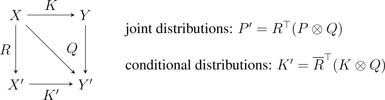
To sum up, if we combine the transformations due to Q and R, then the joint probability distribution transforms as P ⟼ R^⊤ (P ⊗ Q) and the conditional transforms as $K\mapsto {\overline{R}}^{{}^{\top }}\left(K\otimes Q\right)$. In particular, for the joint distribution, we obtain the definition of a Lebanon map. Figure 1 illustrates the situation.

Finally, we will also consider the special case where the partition of R (and $\overline{R}$) is homogeneous, i.e., such that all blocks have the same size. For example, this describes the case where there is a third random variable Z that is independent of Y given X. In this case, the conditional distribution satisfies P(Y|X) = P(Y|X, Z), and R describes the conditional distribution of (X, Z) given X.

Definition 9. A (row) partition indicator matrix is a matrix $\overline{R}\in {\left\{0,1\right\}}^{k\times l}$ that satisfies:

$${\overline{R}}_{ij}=\{\begin{array}{ll}1,\hfill & ifj\in A_i,\hfill \\ 0,\hfill & \text{else},\hfill \end{array}$$

(20)

for a k block partition {A₁,…, A_k} of [l].

For example, the 3 × 5 partition indicator matrix corresponding to Equation (8) is:

$$\overline{R}=\left(\begin{array}{lllll}1\hfill & 0\hfill & 1\hfill & 0\hfill & 0\hfill \\ 0\hfill & 1\hfill & 0\hfill & 1\hfill & 0\hfill \\ 0\hfill & 0\hfill & 0\hfill & 0\hfill & 1\hfill \end{array}\right).$$

(21)

Definition 10. Consider a k × l partition indicator matrix $\overline{R}$ and a collection of m × n stochastic partition matrices $Q={\left\{Q^{\left(i\right)}\right\}}_{i=1}^k$. We call the map:

$$f:{\mathrm{ℝ}}_{+}^{k\times m}\to {\mathrm{ℝ}}_{+}^{l\times n};M\mapsto {\overline{R}}^{\top }\left(M\otimes Q\right)$$

(22)

a conditional embedding of ${\mathrm{ℝ}}_{+}^{k\times m}$ in ${\mathrm{ℝ}}_{+}^{l\times n}$. We denote the set of all such maps by ${\widehat{ℱ}}_{k,m}^{l,n}$. If $\overline{R}$ is the partition indicator matrix of a homogeneous partition (with partition blocks of equal cardinality), then we call f a homogeneous conditional embedding. We denote the set of all such homogeneous conditional embeddings by ${\widehat{ℱ}}_{k,m}^{l,n}$ and assume that l is a multiple of k.

Conditional embeddings preserve the 1-norm of the matrix rows; that is, the elements of ${\widehat{ℱ}}_{k,m}^{l,n}$ map $\left({\mathrm{\Delta }}_{m-1}^k\right)°$ to $\left({\mathrm{\Delta }}_{n-1}^k\right)°$. On the other hand, they do not preserve the 1-norm of the entire matrix. Conditional embeddings are Markov maps only when k = l, in which case they are also Lebanon maps.

4.2. Invariance Characterization

Considering the conditional embeddings discussed in the previous section, we obtain the following metric characterization.

Theorem 11.

• Let g^(k,m) denote a metric on${\mathrm{ℝ}}_{+}^{k\times m}$ for each k ≥ 1 and m ≥ 2. If every homogeneous conditional embedding$f\in {ℱ}_{k,m}^{l,n}$ is an isometry with respect to these metrics, then:

  $$g_M^{\left(k,m\right)}\left({\partial }_{ab},{\partial }_{cd}\right)=\frac{A}{k^2}+{\delta }_{ac}\left(k\frac{B}{k^2}+{\delta }_{bd}\frac{\left|M\right|}{M_{ab}}\frac{C}{k^2}\right),forallM\in {\mathrm{ℝ}}_{+}^{k\times m},$$

  (23)

  for some constants$A,B,C\in \mathrm{ℝ}$, where${\partial }_{ab}=\frac{\partial }{\partial M_{ab}}$ and$\left|M\right|={\displaystyle {\sum }_{ab}{M}_{ab}}$.

• Conversely, given the metrics defined by Equation (23) for any non-degenerate choice of constants$A,B,C\in \mathrm{ℝ}$, each homogeneous conditional embedding$f\in {ℱ}_{k,m}^{l,n},k\le l,m\le n$ is an isometry.

• Moreover, the tensors g^(k,m) from Equation (23) are positive-definite for all k ≥ 1 and m ≥ 2 if and only if C > 0, B + C > 0 and A + B + C > 0.

The proof of Theorem 11 is similar to the proof of the theorems of Chentsov, Campbell and Lebanon. Due to its technical nature, we defer it to Appendix B.

Now, for the restriction of the metric g^(k,m) to $\left({\mathrm{\Delta }}_{m-1}^k\right)°$, we have the following. In this case, |M| = k. Since tangent vectors $\upsilon ={\displaystyle {\sum }_{ab}{\upsilon }_{ab}{\partial }_{ab}\in T_M\left({\mathrm{\Delta }}_{m-1}^k\right)°}$ satisfy ${\displaystyle {\sum }_b{\upsilon }_{ab}}=0$ for all a, the constants A and B become immaterial, and the metric can be written as:

$$g_M^{\left(k,m\right)}\left(u,\upsilon \right)={\displaystyle \sum _{ab}\frac{\left|M\right|u_{ab}{\upsilon }_{ab}}{M_{ab}}\frac{C}{k^2}={\displaystyle \sum _{ab}\frac{u_{ab}{\upsilon }_{ab}}{M_{ab}}\frac{C}{k},\text{for all }u,\upsilon \in T_M({\mathrm{\Delta }}_{m-1}^k)°.}}$$

(24)

This metric is a specialization of the metric (18) derived by Lebanon (Theorem 6).

The statement of Theorem 11 becomes false if we consider general conditional embeddings instead of homogeneous ones:

Theorem 12. There is no family of metrics g^(k,m) on${\mathrm{ℝ}}_{+}^{k\times m}$ (or on$\left({\mathrm{\Delta }}_{m-1}^k\right)°$) for each k ≥ 1 and m ≥ 2, for which every conditional embedding$f\in {\widehat{ℱ}}_{k,m}^{l,n}$ is an isometry.

This negative result will become clearer from the perspective of Section 6: as we will show in Theorem 17, although there are no metrics that are invariant under all conditional embeddings, there are families of metrics (depending on a parameter, ρ) that transform covariantly (that is, in a well-defined manner) with respect to the conditional embeddings. We defer the proof of Theorem 12 to Appendix B.

5. The Fisher Metric on Polytopes and Point Configurations

In the previous section, we obtained distinguished Riemannian metrics on ${\mathrm{ℝ}}_{+}^{k\times m}$ and $\left({\mathrm{\Delta }}_{m-1}^k\right)°$ by postulating invariance under natural maps. In this section, we take another viewpoint based on general considerations about Riemannian metrics on arbitrary polytopes. This is achieved by embedding each polytope in a probability simplex as an exponential family. We first recall the necessary background. In Section 5.2, we then present our general results, and in Section 5.3, we discuss the special case of conditional polytopes.

5.1. Exponential Families and Polytopes

Let $\mathcal{X}$ be a finite set and $A\in {\mathrm{ℝ}}^{d\times \mathcal{X}}$ a matrix with columns a_x indexed by $x\in \mathcal{X}$. It will be convenient to consider the rows A_i, i ∈ [d] of A as functions $A_i:\mathcal{X}\to \mathrm{ℝ}$ Finally, let $\nu :\mathcal{X}\to {\mathrm{ℝ}}_{+}$. The exponential family ε_A,ν is the set of probability distributions on $\mathcal{X}$ given by:

$$p\left(x;\theta \right)=\exp \left({\theta }^{\top }{a}_x+\log \left(\nu \left(x\right)\right)-\log \left(Z\left(\theta \right)\right)\right),\text{for all }x\in \mathcal{X},\text{for all }\theta \in {\mathrm{ℝ}}^d,$$

(25)

with the normalization function $Z\left(\theta \right)={\displaystyle {\sum }_{x^{\prime }\in \mathcal{X}}\exp \left({\theta }^{\top }{a}_{x^{\prime }}+\log \left(\nu \left(x^{\prime }\right)\right)\right)}$. The functions A_i are called the observables and ν the reference measure of the exponential family. When the reference measure ν is constant, ν(x) = 1 for all $x\in \mathcal{X}$, we omit the subscript and write ε_A.

A direct calculation shows that the Fisher information matrix of ε_A,_ν at a point $\theta \in {\mathrm{ℝ}}^d$ has coordinates:

$$g_{\theta }^{{\epsilon }_{A,\nu }}({\partial }_{{\theta }_i},{\partial }_{{\theta }_j})={\text{cov}}_{\theta }(A_i,A_j),\text{\hspace{0.17em}for all} i,j\in [d].$$

(26)

Here, cov_θ denotes the covariance computed with respect to the probability distribution p(·; θ).

The convex support of ε_A,_ν is defined as:

(27)

where conv S is the set of all convex combinations of points in S. The moment map $\mu :p\in {\mathrm{\Delta }}_{n-1}\mapsto A·p\in {\mathrm{ℝ}}^d$ restricts to a homeomorphism $\overline{{\epsilon }_{A,v}}\to \text{conv }A$ conv A; see [16]. Here, $\overline{{\epsilon }_{A,v}}$ denotes the Euclidean closure of ε_A,ν. The inverse of μ will be denoted by ${\mu }^{-1}:\text{conv }A\to \overline{{\epsilon }_{A,v}}\subseteq {\mathrm{\Delta }}_{n-1}$. This gives a natural embedding of the polytope conv A in the probability simplex ${\mathrm{\Delta }}_{\left|\mathcal{X}\right|-1}$. Note that the convex support is independent of the reference measure ν. See [17] for more details.

5.2. Invariance Fisher Metric Characterizations for Polytopes

Let $\mathrm{P}\in {\mathrm{ℝ}}^d$ be a polytope with n vertices a₁,…, a_n. Let A = (a₁,…, a_n) be the matrix with columns $a_i\in {\mathrm{ℝ}}^d$ for all i ∈ [n]. Then, ${\epsilon }_A\subseteq {\mathrm{\Delta }}_{n-1}^{\circ }$ is an exponential family with convex support P. We will also denote this exponential family by ε_P. We can use the inverse of the moment map, μ⁻¹, to pull back geometric structures on ${\mathrm{\Delta }}_{n-1}^{\circ }$ to the relative interior P° of P.

Definition 13. The Fisher metric on P° is the pull-back of the Fisher metric on ${\epsilon }_A\subseteq {\mathrm{\Delta }}_{n-1}^{\circ }$ by μ⁻¹.

Some obvious questions are: Why is this a natural construction? Which maps between polytopes are isometries between their Fisher metrics? Can we find a characterization of Chentsov type for this metric?

Affine maps are natural maps between polytopes. However, in order to obtain isometries, we need to put some additional constraints. Consider two polytopes $\mathrm{P}\in {\mathrm{ℝ}}^d$, ${\mathrm{P}}^{\prime }\in {\mathrm{ℝ}}^d{}^{\prime }$ and an affine map $\varphi :{\mathrm{ℝ}}^d\to {\mathrm{ℝ}}^d{}^{\prime }$ that satisfies ϕ(P) ⊆ P′. A natural condition in the context of exponential families is that ϕ restricts to a bijection between the set vert(P) of vertices of P and the set vert(P′) of vertices of P′. In this case, ${\epsilon }_{{\mathrm{P}}^{\prime }}\subseteq {\epsilon }_{{\mathrm{P}}^{\prime }}\subseteq {\mathrm{\Delta }}_{n-1}^{\circ }$. Moreover, the moment map μ′ of P′ factorizes through the moment map μ of P: μ′ = ϕ ○ μ. Let ϕ⁻¹ = μ ○ μ^′−1. Then, the following diagram commutes:

(28)

It follows that ϕ⁻¹ is an isometry from P′° to its image in P°. Observe that the inverse moment map itself arises in this way: In the diagram (28), if P is equal to ∆_n−1, then the upper moment map μ⁻¹ is the identity map, and ϕ⁻¹ equals the inverse moment map μ'⁻¹ of P′.

The constraint of mapping vertices to vertices bijectively is very restrictive. In order to consider a larger class of affine maps, we need to generalize our construction from polytopes to weighted point configurations.

Definition 14. A weighted point configuration is a pair (A, ν) consisting of a matrix $A\times {\mathrm{ℝ}}^{d\times n}$ with columns a₁,…, a_n and a positive weight function $\nu :\left\{1,\dots ,n\right\}\to {\mathrm{ℝ}}_{+}$ assigning a weight to each column a_i. The pair (A, ν) defines the exponential family ε_A,_ν.

The (A, ν)-Fisher metric on (conv A)° is the pull-back of the Fisher metric on ${\mathrm{\Delta }}_{n-1}^{\circ }$ through the inverse of the moment map.

We recover Definition 13 as follows. For a polytope P, let A be the point configuration consisting of the vertices of P. Moreover, let ν be a constant function. Then, ε_P = ε_A,_ν, and the two definitions of the Fisher metric on P° coincide.

The following are natural maps between weighted point configurations:

Definition 15. Let (A, ν), (A′, ν′) be two weighted point configurations with $A={\left(a_i\right)}_i\in {\mathrm{ℝ}}^{d\times n}$ and $A^{\prime }={({a^{\prime }}_j)}_j\in {\mathrm{ℝ}}^{d^{\prime }\times n^{\prime }}$. A morphism (A,ν) → (A′,ν′) is a pair (ϕ, σ) consisting of an affine map $\varphi :{\mathrm{ℝ}}^d\to {\mathrm{ℝ}}^{d^{\prime }}$ and a surjective map σ: {1,…, n} → {1,…, n′} with $\varphi \left(a_i\right)={a^{\prime }}_{\sigma \left(i\right)}$ and $v^{\prime }\left({a^{\prime }}_j\right)=\alpha {\displaystyle {\sum }_{i:\sigma \left(i\right)=j}v\left(a_i\right)}$, where α > 0 is a constant that does not depend on j.

Consider a morphism (ϕ, σ): (A, ν) → (A′, ν′). For each j ∈ [n′], let $A_j=\left\{i:\varphi \left(a_i\right)={a^{\prime }}_j\right\}$. Then, is $\left(A_1,\dots ,A_{n^{\prime }}\right)$ a partition of [n]. Define a matrix $Q\in {\mathrm{ℝ}}^{n^{\prime }\times n}$ by:

$$Q_{ji}=\{\begin{array}{ll}\frac{\nu \left(i\right)}{{\displaystyle {\sum }_{i^{\prime }\in A_j}\nu \left(i^{\prime }\right)}},\hfill & \text{if }i\in A_j,\hfill \\ 0,\hfill & \text{else}.\hfill \end{array}$$

(29)

Then, Q is a Markov mapping, and the following diagram commutes:

(30)

By Chentsov’s theorem (Theorem 2), Q is an isometric embedding. It follows that ϕ⁻¹ also induces an isometric embedding. This shows the first part of the following theorem:

Theorem 16.

• Let (ϕ, σ): (A, ν) → (A′, ν′) be a morphism of weighted point configurations. Then, ϕ⁻¹: (conv A′)° → (conv A)° is an isometric embedding with respect to the Fisher metrics on (conv A)° and (conv A')°.

• Let g^A,^ν be a Riemannian metric on (conv A)° for each weighted point configuration (A, ν). If every morphism (ϕ, σ): (A, ν) → (A′, ν′) of weighted point configurations induces an isometric embedding ϕ⁻¹: (convA′)° → (conv A)°, then there exists a constant$\alpha \in {\mathrm{ℝ}}_{+}$ such that g^A,^ν is equal to α times the (A, ν)-Fisher metric.

Proof. The first statement follows from the discussion before the theorem. For the second statement, we show that under the given assumptions, all Markov maps are isometric embeddings. By Chentsov’s theorem (Theorem 2), this implies that the metrics g^P agree with the Fisher metric whenever P is a simplex. The statement then follows from the two facts that the metric on P° or (conv A)° is the pull-back of the Fisher metric through the inverse of the moment map and that μ⁻¹ is itself a morphism.

Observe that ∆_n−1 = conv I_n = conv{e₁,…, e_n} is a polytope, and ${\mathrm{\Delta }}_{n-1}^{\circ }$ is the corresponding exponential family. Consider a Markov embedding $Q:{\mathrm{\Delta }}_{n^{\prime }-1}^{\circ }\to {\mathrm{\Delta }}_{n-1}^{\circ }$, p ⟼ p·· Q. Let $\nu \left(i\right)={\displaystyle {\sum }_j{Q}_{ji}}$ be the value of the unique non-zero entry of Q in the i-th column. This defines a morphism and an embedding as follows:

Let A be the matrix that arises from Q by replacing each non-zero entry by one. We define ϕ as the linear map represented by the matrix A, and define σ: [n] → [n'] by σ(j) = i if and only if a_j = e_i, that is, σ(j) indicates the row i in which the j-th column of A is non-zero. Then, (ϕ, σ) is a morphism $\left(I_n,\nu \right)\to \left(I_{n^{\prime }},1\right)$, and by assumption, the inverse ϕ⁻¹ is an isometric embedding ${\mathrm{\Delta }}_{n^{\prime }-1}^{\circ }\to {\mathrm{\Delta }}_{n-1}^{\circ }$. However, ϕ⁻¹ is equal to the Markov map Q. This shows that all Markov maps are isometric embeddings, and so, by Chentsov’s theorem, the statement holds true on the simplices. □

Theorem 16 defines a natural metric on $\left({\mathrm{\Delta }}_{m-1}^k\right)°$ that we want to discuss in more detail next.

5.3. Independence Models and Conditional Polytopes

Consider k random variables with finite state spaces [n₁],…, [n_k]. The independence model consists of all joint distributions $p\in {\mathrm{\Delta }}_{{\displaystyle {\prod }_{i\in \left[k\right]}{n}_i-1}}$ of these variables that factorize as:

$$p\left(x_1,\dots ,x_k\right)={\displaystyle \prod _{i\in \left[k\right]}{p}_i\left(x_i\right),\text{for all }{x}_1\in \left[n_1\right],\dots ,x_k\in \left[n_k\right],}$$

(31)

where $p_i\in {\mathrm{\Delta }}_{n_i-1}$ for all i ∈ [k]. Assuming fixed n₁,…, n_k, we denote the independence model by $\overline{{\epsilon }_k}$. It is the Euclidean closure of an exponential family (with observables of the form ${\delta }_{i{y}_i}$). The convex support of ε_k is equal to the product of simplices ${\mathrm{P}}_k:={\mathrm{\Delta }}_{n_1-1}\times \cdots \times {\mathrm{\Delta }}_{n_k-1}$. The parametrization (31) corresponds to the inverse of the moment map.

We can write any tangent vector $u\in T_{(p_1,\dots ,p_k)}{\mathrm{P}}_k^{\circ }$ of this open product of simplices as a linear combination $u={\displaystyle {\sum }_{i\in \left[k\right]}{\displaystyle {\sum }_{x_i\in \left[n_i\right]}{u}_{i{x}_i}{\partial }_{i,x_i}}}$, where ${\displaystyle {\sum }_{x_i\in \left[n_i\right]}{\upsilon }_{i{x}_i}}=0$ for all i ∈ [k]. Given two such tangent vectors, the Fisher metric is given by:

$$g_{\left(p_1,\dots ,p_k\right)}^{{\mathrm{P}}_k}\left(u,\upsilon \right)={\displaystyle \sum _{i\in \left[k\right]}{\displaystyle \sum _{x_i\in \left[n_i\right]}\frac{u_{i{x}_i}{\upsilon }_{i{x}_i}}{p_i\left(x_i\right)}}}$$

(32)

Just as the convex support of the independence model is the Cartesian product of probability simplices, the Fisher metric on the independence model is the product metric of the Fisher metrics on the probability simplices of the individual variables. If n₁ = … = n_k =: n, then ${\mathrm{P}}_k={\mathrm{\Delta }}_{n-1}^k$ can be identified with the set of k × n stochastic matrices.

The Fisher metric on the product of simplices is equal to the product of the Fisher metrics on the factors. More generally, if P = Q₁ × Q₂ is a Cartesian product, then the Fisher metric on P° is equal to the product of the Fisher metrics on ${\mathrm{Q}}_1^{\circ }$ and ${\mathrm{Q}}_2^{\circ }$. In fact, in this case, the inverse of the moment map of P can be expressed in terms of the two moment map inverses ${\mu }_1:{\mathrm{Q}}_1\to \overline{{\epsilon }_{{\mathrm{Q}}_1}}\subseteq {\mathrm{\Delta }}_{m_1-1}$ and ${\mu }_2:{\mathrm{Q}}_2\to \overline{{\epsilon }_{{\mathrm{Q}}_2}}\subseteq {\mathrm{\Delta }}_{m_2-1}$ and the moment map $\tilde{\mu }$ of the independence model ${\mathrm{\Delta }}_{m_1-1}\times {\mathrm{\Delta }}_{m_2-1}$, by:

$${\mu }^{-1}\left(q_1,q_2\right)={\tilde{\mu }}^{-1}\left({\mu }_1^{-1}\left(q_1\right),{\mu }_2^{-1}\left(q_2\right)\right).$$

(33)

Therefore, the pull-back by μ⁻¹ factorizes through the pull-back by ${\tilde{\mu }}^{-1}$, and since the independence model carries a product metric, the product of polytopes also carries a product metric.

Let us compare the metric $g_K^{\left(k,m\right)}$ from Equation (24), with the Fisher metric $g_{\left(K_1,\dots ,K_k\right)}^{{\mathrm{P}}_k}$ from Equation (32) on the product of simplices ${\mathrm{P}}^{\circ }={\left({\mathrm{\Delta }}_{m-1}^k\right)}^{\circ }$. In both cases, the metric is a product metric; that is, it has the form:

$$g=g_1+\cdots +g_k,$$

(34)

where g_i is a metric on the i-th factor ${\mathrm{\Delta }}_{m-1}^{\circ }$. For $g_K^{{\mathrm{\Delta }}_{m-1}^k}$, g_i is equal to the Fisher metric on ${\mathrm{\Delta }}_{m-1}^{\circ }$. However, for $g_K^{\left(k,m\right)}$, g_i is equal to 1/k times the Fisher metric on ${\mathrm{\Delta }}_{m-1}^{\circ }$. Since this factor only depends on k, it only plays a role if stochastic matrices of different sizes are compared. The additional factor of 1/k can be interpreted as the uniform distribution on k elements. This is related to another more general class of Riemannian metrics that are used in applications; namely, given a function $K\in {\mathrm{\Delta }}_{m-1}^k\to {\rho }^K\in {\mathrm{ℝ}}_{+}^k$, it is common to use product metrics with g_i equal to ρ^K(i) times the Fisher metric on ${\mathrm{\Delta }}_{m-1}^{\circ }$. When K has the interpretation of a channel or when K describes the policy by which a system reacts to some sensor values, a natural possibility is to let ρ^K be the stationary distribution of the channel input or of the sensor values, respectively. We will discuss this approach in Section 6.

6. Weighted Product Metrics for Conditional Models

In this section, we consider metrics on spaces of stochastic matrices defined as weighted sums of the Fisher metrics on the spaces of the matrix rows, similar to Equation (34). This kind of metric was used initially by Amari [1] in order to define a natural gradient in the supervised learning context. Later, in the context of reinforcement learning, Kakade [2] defined a natural policy gradient based on this kind of metric, which has been further developed by Peters et al. [10]. Related applications within unsupervised learning have been pursued by Zahedi et al. [18].

Consider the following weighted product Fisher metric:

$$g_K^{\rho ,m}={\displaystyle \sum _a{\rho }^K\left(a\right)g_{K_a}^{\left(m\right),a},\text{for all }K\in \left({\mathrm{\Delta }}_{m-1}^k\right)°,}$$

(35)

where $g_{K_a}^{\left(m\right),a}$ denotes the Fisher metric of ${\mathrm{\Delta }}_{m-1}^{\circ }$ at the a-th row of K and ${\rho }^K\in {\mathrm{\Delta }}_{k-1}^{\circ }$ is a probability distribution over a associated with each $K\in \left({\mathrm{\Delta }}_{m-1}^k\right)°$. For example, the distribution ρ^K could be the stationary distribution of sensor values observed by an agent when operating under a policy described by K.

In the following, we will try to illuminate the properties of polytope embeddings that yield the metric (35) as the pull-back of the Fisher information metric on a probability simplex. We will focus on the case that ρ^K = ρ is independent of K.

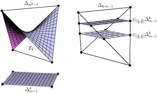
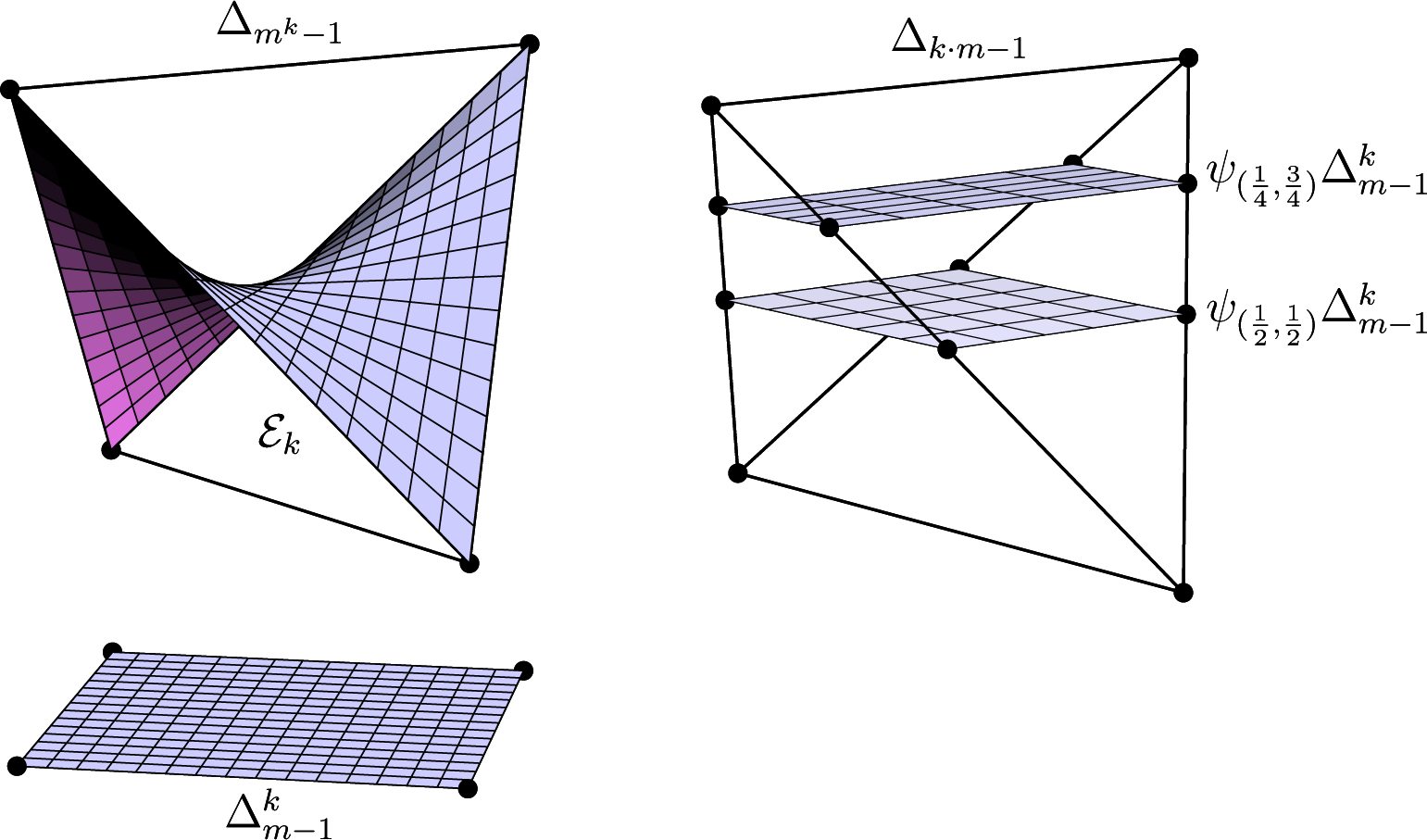
There are two direct ways of embedding ${\mathrm{\Delta }}_{n-1}^k$ in a probability simplex. In Section 5, we used the inverse of the moment map of an exponential family, possibly with some reference measure. This embedding is illustrated in the left panel of Figure 2. If we have given a fixed probability distribution $\rho \in {\mathrm{\Delta }}_{k-1}^{\circ }$, there is a second natural embedding ${\psi }_{\rho }:{\mathrm{\Delta }}_{m-1}^k\to {\mathrm{\Delta }}_{k\cdot m-1}$ defined as follows:

$${\psi }_{\rho }\left(K\right)\left(x,y\right)=\rho \left(x\right)K_{x,y}\text{for all }x\in \left[k\right],y\in \left[m\right].$$

(36)

If ρ is the distribution of a random variable X and $K\in {\mathrm{\Delta }}_{m-1}^k$ is the stochastic matrix describing the conditional distribution of another variable Y given X, then ψ_ρ(K) is the joint distribution of X and Y. Note that ψ_ρ is an affine embedding. See the right panel of Figure 2 for an illustration.

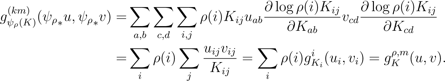
The pull-back of the Fisher metric on ${\mathrm{\Delta }}_{km-1}^{\circ }$ through ψ_ρ is given by:

(37)

This recovers the weighted sum of Fisher metrics from Equation (35).

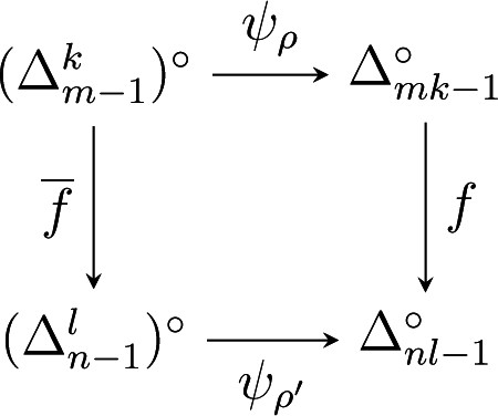
Are there natural maps that leave the metrics g^ρ,^m invariant? Let us reconsider the stochastic embeddings from Definition 10. Let $\overline{R}$ be a k × l indicator partition matrix and R a stochastic partition matrix with the same block structure as $\overline{R}$. Observe that to each indicator partition matrix $\overline{R}$ there are many compatible stochastic partition matrices R, but the indicator partition matrix $\overline{R}$ for any stochastic partition matrix R is unique. Furthermore, let Q = {Q^(a)}_a∈[k] be a collection of stochastic partition matrices. The corresponding conditional embedding $\overline{f}$ maps $K\in {\mathrm{\Delta }}_{m-1}^k$ to $\overline{f}\left(K\right):{\overline{R}}^{\top }\left(K\otimes Q\right)\in {\mathrm{\Delta }}_{n-1}^l$.

Let $\rho \in {\mathrm{\Delta }}_{k-1}^{\circ }$. Suppose that K describes the conditional distribution of Y given X and that ψ_ρ(K) describes the joint distribution of Y and X. As explained in Section 4.1, the matrix f(P) := R^⊤(P⊗Q) describes the joint distribution of a pair of random variables (X′, Y′), and the conditional distribution of Y′ given X′ is given by $\overline{f}\left(K\right)$. In this situation, the marginal distribution of X′ is given by ρ′ = ρR. Therefore, the following diagram commutes:

(38)

The preceding discussion implies the first statement of the following result:

Theorem 17.

• For any k ≥ 1 and m ≥ 2 and any $\rho \in {\mathrm{\Delta }}_{k-1}^{\circ }$, the Riemannian metric g^ρ,^m on$\left({\mathrm{\Delta }}_{m-1}^k\right)°$ satisfies:

  $$g^{\rho ,m}={\overline{f}}^{*}\left(g^{{\rho }^{\prime },n}\right),for{\rho }^{\prime }=\rho R,$$

  (39)

  for any conditional embedding$\overline{f}:K\mapsto \overline{R}\left(K\otimes Q\right)$.

• Conversely, suppose that for any k ≥ 1 and m ≥ 2 and any$\rho \in {\mathrm{\Delta }}_{k-1}^{\circ }$, there is a Riemannian metric g^(ρ,m) on$\left({\mathrm{\Delta }}_{m-1}^k\right)°$, such that Equation (39) holds for all conditional embeddings, and suppose that g^(ρ,m) depends continuously on ρ. Then, there is a constant A > 0 that satisfies g^(ρ,m) = Ag^ρ,^m.

Proof. The first statement follows from the commutative diagram (38). For the second statement, denote by ρ^k the uniform distribution on a set of k elements. If $\overline{f}:K\mapsto \overline{R}\left(K\otimes Q\right)$ is a homogeneous conditional embedding of ${\mathrm{\Delta }}_{m-1}^k$ in ${\mathrm{\Delta }}_{n-1}^l$, then $R=\frac{k}{l}\overline{R}$ is a stochastic partition matrix corresponding to the partition indicator matrix $\overline{R}$. Observe that ρ^l = ρ^kR. Therefore, the family of Riemannian metrics $g^{{\rho }^k,m}$ on ${\mathrm{\Delta }}_{m-1}^k$ satisfies the assumptions of Theorem 11. Therefore, there is a constant A > 0 for which $g^{{\rho }^k,m}$ equals A/k times the product Fisher metric. This proves the statement for uniform distributions ρ.

A general distribution $\rho \in {\mathrm{\Delta }}_{k-1}^{\circ }$ can be approximated by a distribution with rational probabilities. Since g^(ρ,m) is assumed to be continuous, it suffices to prove the statement for rational ρ. In this case, there exists a stochastic partition matrix R for which ρ′ := ρR is a uniform distribution, and so, $g^{\left({\rho }^{\prime },n\right)}$ is of the desired form. Equation (39) shows that g^(ρ,m) is also of the desired form. □

7. Gradient Fields and Replicator Equations

In this section, we use gradient fields in order to compare Riemannian metrics on the space $\left({\mathrm{\Delta }}_{n-1}^k\right)°$.

7.1. Replicator Equations

We start with gradient fields on the simplex ${\mathrm{\Delta }}_{n-1}^{\circ }$. A Riemannian metric g on ${\mathrm{\Delta }}_{n-1}^{\circ }$ allows us to consider gradient fields of differentiable functions $F:{\mathrm{\Delta }}_{n-1}^{\circ }\to \mathrm{ℝ}$. To be more precise, consider the differential $d_{p}F:T_p{\mathrm{\Delta }}_{n-1}^{\circ }\to \mathrm{ℝ}$ of F in p. It is a linear form on $T_p{\mathrm{\Delta }}_{n-1}^{\circ }$, which maps each tangent vector u to $d_{p}F\left(u\right)=\frac{\partial F}{\partial u}\left(p\right)\in \mathrm{ℝ}$. Using the map u ⟼ g_p(u, ·), this linear form can be identified with a tangent vector in $T_p{\mathrm{\Delta }}_{n-1}^{\circ }$, which we denote by grad_pF. If we choose the Fisher metric g⁽ⁿ⁾ as the Riemannian metric, we obtain the gradient in the following way. First consider a differentiable extension of F to the positive cone ${\mathrm{ℝ}}_{+}^n$, which we will denote by the same symbol F. With the partial derivatives ∂_iF of F, the Fisher gradient of F on the simplex ${\mathrm{\Delta }}_{n-1}^{\circ }$ is given as:

$${\left({\text{grad}}_{p}F\right)}_i=p_i\left({\partial }_{i}F\left(p\right)-{\displaystyle \sum _{j=1}^n{p}_j}{\partial }_{j}F\left(p\right)\right),i\in \left[n\right].$$

(40)

Note that the expression on the right-hand side of Equation (40) does not depend on the particular differentiable extension of F to ${\mathrm{ℝ}}_{+}^n$. The corresponding differential equation is well known in theoretical biology as the replicator equation; see [19,20].

$${\dot{p}}_i=p_i\left({\partial }_{i}F\left(p\right)-{\displaystyle \sum _{j=1}^n{p}_j}{\partial }_{j}F\left(p\right)\right),i\in \left[n\right].$$

(41)

We now apply this gradient formula to functions that have the structure of an expectation value. Given real numbers Fi, i ∈ [n], referred to as fitness values, we consider the mean fitness:

$$\overline{F}\left(p\right):={\displaystyle \sum _{i=1}^n{p}_i{F}_i.}$$

(42)

Replacing the p_i by any positive real numbers leads to a differentiable extension of F, also denoted by F. Obviously, we have ∂_iF = F_i, which leads to the following replicator equation:

$${\dot{p}}_i=p_i\left(F_i-\overline{F}\left(p\right)\right),i\in \left[n\right].$$

(43)

This equation has the solution:

$$p_i\left(t\right)=\frac{p_i\left(0\right)e^{t{F}_i}}{{\displaystyle {\sum }_{j=1}^n{p}_j\left(0\right)e^{t{F}_i}}},i\in \left[n\right].$$

(44)

Clearly, the mean fitness will increase along this solution of the gradient field. The rate of increase can be easily calculated:

$$\frac{d}{dt}\overline{F}\left(p\left(t\right)\right)={\displaystyle \sum _{i=1}^n{\dot{p}}_i\left(t\right)F_i}={\displaystyle \sum _{i=1}^n{p}_i\left(F_i-\overline{F}\left(p\right)\right)F_i}={\displaystyle \sum _{i=1}^n{p}_i{\left(F_i-\overline{F}\left(p\right)\right)}^2={\mathrm{var}}_p\left(F\right)>0.}$$

(45)

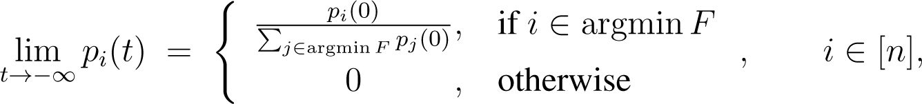
As limit points of this solution, we obtain:

(46)

and:

(47)

7.2. Extension of the Replicator Equations to Stochastic Matrices

Now, we come to the corresponding considerations of gradient fields in the context of stochastic matrices $K\in \left({\mathrm{\Delta }}_{n-1}^k\right)°$. We consider a function:

$$K\mapsto F\left(K\right)=F\left(K_{11},\dots ,K_{1n};K_{21},\dots ,K_{2n};\dots ;K_{k1},\dots ,K_{kn}\right).$$

(48)

One way to deal with this is to consider for each i ∈ [k] the corresponding replicator equation:

$${\dot{K}}_{ij}=K_{ij}\left({\partial }_{ij}F\left(K\right)-{\displaystyle \sum _{j^{\prime }=1}^n{k}_{i{j}^{\prime }}{\partial }_{i{j}^{\prime }}F\left(K\right)}\right),j\in \left[n\right].$$

(49)

Obviously, this is the gradient field that one obtains by using the product Fisher metric on $\left({\mathrm{\Delta }}_{n-1}^k\right)°$ (Equation (17)):

$$g_K^{(k,m)}(u,\upsilon )={\displaystyle \sum _{ij}\frac{1}{K_{ij}}{u}_{ij}{\upsilon }_{ij}.}$$

(50)

If we replace the metric by the weighted product Fisher metric considered by Kakade (Equation (35)),

$$g_K^{\rho ,m}\left(u,\upsilon \right)={\displaystyle \sum _{ij}\frac{{\rho }_i}{K_{ij}}{u}_{ij}{\upsilon }_{ij},}$$

(51)

then we obtain

$${\dot{K}}_{ij}=\frac{K_{ij}}{{\rho }_i}\left({\partial }_{ij}F\left(K\right)-{\displaystyle \sum _{j^{\prime }=1}^n{K}_{i{j}^{\prime }}{\partial }_{i{j}^{\prime }}F\left(K\right)}\right),j\in \left[n\right].$$

(52)

7.3. The Example of Mean Fitness

Next, we want to study how the gradient flows with respect to different metrics compare. We restrict to the class of metrics g^ρ,^m (Equation (35)), where $\rho \in {\mathrm{\Delta }}_k^{\circ }$ is a probability distribution. In principle, one could drop the normalization condition ${\sum }_i{\rho }_i=1$ and allow arbitrary coefficients ρ_i. However, it is clear that the rate of convergence can always be increased by scaling all values ρ_i with a common positive factor. Therefore, some normalization condition is needed for ρ.

With a probability distribution $\rho \in {\mathrm{\Delta }}_{k-1}^{\circ }$ and fitness values F_ij, let us consider again the example of an expectation value function:

$$\overline{F}\left(K\right)={\displaystyle \sum _{i=1}^k{p}_i}{\displaystyle \sum _{j=1}^n{K}_{ij}{F}_{in}.}$$

(53)

With ${\partial }_{ij}\overline{F}\left(\pi \right)=p_i{F}_{ij}$, this leads to:

$${\dot{K}}_{ij}=\frac{p_i}{{\rho }_i}{K}_{ij}\left(F_{ij}-{\displaystyle \sum _{j^{\prime }=1}^n{K}_{i{j}^{\prime }}{F}_{i{j}^{\prime }}}\right),j\in \left[n\right].$$

(54)

The corresponding solutions are given by:

$$K_{ij}\left(t\right)=\frac{K_{ij}\left(0\right)e^{t\frac{P_i}{{\rho }_i}{F}_{ij}}}{{\displaystyle {\sum }_{j^{\prime }=1}^n{K}_{i{j}^{\prime }}\left(0\right)e^{t\frac{P_i}{{\rho }_i}{F}_{i{j}^{\prime }}}}},i\in \left[n\right].$$

(55)

Since $\text{argmax}\left(\frac{p_i}{{\rho }_i}{F}_i.\right)$ and $\text{argmin}\left(\frac{p_i}{{\rho }_i}{F}_i.\right)$ are independent of ρ_i > 0, the limit points are given independently of the chosen ρ as:

(56)

and:

(57)

This is consistent with the fact that the critical points of gradient fields are independent of the chosen Riemannian metric. However, the speed of convergence does depend on the metric:

For each i, let G_i = max_j F_ij and $g_i={max}_{j\notin \text{argmax}\left(F_{ij}\right)}{F}_{ij}$ be the largest and second-largest values in the i-th row of F_ij, respectively. Then, as: t → ∞,

(58)

Therefore,

(59)

Thus, in the long run, the rate of convergence is given by ${\text{inf}}_i\left\{\frac{p_i}{{\rho }_i}\left(G_i-g_i\right)\right\}$, which depends on the parameter ρ of the metric. As a result, in this case study, the optimal choice of ρ_i, i.e., with the largest convergence rate, can be computed if the numbers G_i and g_i are known.

Consider, for example, the case that the differences G_i – g_i are of comparable sizes for all i. Then, we need to find the choice of ρ that maximizes ${\text{inf}}_i\left\{\frac{p_i}{{\rho }_i}\right\}$. Clearly, ${\text{inf}}_i\left\{\frac{p_i}{{\rho }_i}\right\}\le 1$ (since there is always an index i with p_i ≤ ρ_i). Equality is attained for the choice ρ_i = p_i. Thus, we recover the choice of Kakade.

8. Conclusions

So, which Riemannian metric should one use in practice on the set of stochastic matrices, $\left({\mathrm{\Delta }}_{n-1}^k\right)°$? The results provided in this manuscript give different answers, depending on the approach. In all cases, the characterized Riemannian metrics are products of Fisher metrics with suitable factor weights. Theorem 11 suggests to use a factor weight proportional to 1/k, and Theorem 16 suggests to use a constant weight independent of k. In many cases, it is possible to work within a single conditional polytope $\left({\mathrm{\Delta }}_{n-1}^k\right)°$ and a fixed k, and then, these two results are basically equivalent. On the other hand, Theorem 17 gives an answer that allows arbitrary factor weights ρ.

Which metric performs best obviously depends on the concrete application. The first observation is that in order to use the metric g^ρ,^m of Theorem 17, it is necessary to know ρ. If the problem at hand suggests a natural marginal distribution ρ, then it is natural to make use of it and choose the metric g^ρ,^m. Even if ρ is not known at the beginning, a learning system might try to learn it to improve its performance.

On the other hand, there may be situations where there is no natural choice of the weights ρ. Observe that ρ breaks the symmetry of permuting the rows of a stochastic matrix. This is also expressed by the structural difference between Theorems 11 and 16 on the one side and Theorem 17 on the other. While the first two theorems provide an invariance metric characterization, Theorem 17 provides a “covariance” classification; that is, the metrics g^ρ,^m are not invariant under conditional embeddings, but they transform in a controlled manner. This again illustrates that the choice of a metric should depend on which mappings are natural to consider, e.g., which mappings describe the symmetries of a given problem.

For example, consider a utility function of the form $F={\displaystyle {\sum }_i{\rho }_i}{\displaystyle {\sum }_j{K}_{ij}{F}_{ij}}$. Row permutations do not leave g^ρ,^m invariant (for a general ρ), but they are not symmetries of the utility function F, either, and hence, they are not very natural mappings to consider. However, row permutations transform the metric g^ρ,^m and the utility function in a controlled manner; in such a way that the two transformations match. Therefore, in this case, it is natural to use g^ρ,^m. On the other hand, when studying problems that are symmetric under all row permutations, it is more natural to use the invariant metric g^(k,m).

References

- Amari, S. Natural gradient works efficiently in learning. Neur. Comput 1998, 10, 251–276. [Google Scholar]
- Kakade, S. A Natural Policy Gradient. In Advances in Neural Information Processing Systems 14; MIT Press: Cambridge, MA, USA, 2001; pp. 1531–1538. [Google Scholar]
- Shahshahani, S. A New Mathematical Framework for the Study of Linkage and Selection; American Mathematical Society: Providence, RI, USA, 1979. [Google Scholar]
- Chentsov, N. Statistical Decision Rules and Optimal Inference; American Mathematical Society: Providence, RI, USA, 1982. [Google Scholar]
- Campbell, L. An extended Čencov characterization of the information metric. Proc. Am. Math. Soc 1986, 98, 135–141. [Google Scholar]
- Sutton, R.S.; McAllester, D.; Singh, S.; Mansour, Y. Policy Gradient Methods for Reinforcement Learning with Function Approximation. In Advances in Neural Information Processing Systems 12; MIT Press: Cambridge, MA, USA, 2000; pp. 1057–1063. [Google Scholar]
- Marbach, P.; Tsitsiklis, J. Simulation-based optimization of Markov reward processes. IEEE Trans. Autom. Control 2001, 46, 191–209. [Google Scholar]
- Montúfar, G.; Ay, N.; Zahedi, K. Expressive power of conditional restricted boltzmann machines for sensorimotor control 2014, arXiv, 1402.3346.
- Ay, N.; Montúfar, G.; Rauh, J. Selection Criteria for Neuromanifolds of Stochastic Dynamics. In Advances in Cognitive Neurodynamics (III); Yamaguchi, Y., Ed.; Springer-Verlag: Dordrecht, The Netherlands, 2013; pp. 147–154. [Google Scholar]
- Peters, J.; Schaal, S. Natural Actor-Critic. Neurocomputing 2008, 71, 1180–1190. [Google Scholar]
- Peters, J.; Schaal, S. Policy Gradient Methods for Robotics, Proceedings of the IEEE International Conference on Intelligent Robotics Systems (IROS 2006), Beijing, China, 9–15 October 2006.
- Peters, J.; Vijayakumar, S.; Schaal, S. Reinforcement learning for humanoid robotics, Proceedings of the third IEEE-RAS international conference on humanoid robots, Karlsruhe, Germany, 29–30 September 2003; pp. 1–20.
- Bagnell, J.A.; Schneider, J. Covariant policy search, Proceedings of the 18th International Joint Conference on Artificial Intelligence, Acapulco, Mexico, August 9–15 2003; Morgan Kaufmann Publishers Inc: San Francisco, CA, USA, 2003; pp. 1019–1024.
- Lebanon, G. Axiomatic geometry of conditional models. IEEE Trans. Inform. Theor 2005, 51, 1283–1294. [Google Scholar]
- Lebanon, G. An Extended Čencov-Campbell Characterization of Conditional Information Geometry, Proceedings of the 20th Conference in Uncertainty in Artificial Intelligence (UAI 04), Banff, AL, Canada, 7–11 July 2004; Chickering, D.M., Halpern, J.Y., Eds.; AUAI Press: Arlington, VA, USA, 2004; pp. 341–345.
- Barndorff-Nielsen, O. Information and Exponential Families: In statistical Theory; John Wiley & Sons, Inc: Hoboken, NJ, USA, 1978. [Google Scholar]
- Brown, L.D. Fundamentals of Statistical Exponential Families with Applications in Statistical Decision Theory; Institute of Mathematical Statistics: Hayward, CA, USA, 1986. [Google Scholar]
- Zahedi, K.; Ay, N.; Der, R. Higher coordination with less control—A result of informaion maximiation in the sensorimotor loop. Adapt. Behav 2010, 18. [Google Scholar]
- Hofbauer, J.; Sigmund, K. Evolutionary Games and Population Dynamics; Cambridge University Press: Cambridge, United Kingdom, 1998. [Google Scholar]
- Ay, N.; Erb, I. On a notion of linear replicator equations. J. Dyn. Differ. Equ 2005, 17, 427–451. [Google Scholar]
© 2014 by the authors; licensee MDPI, Basel, Switzerland This article is an open access article distributed under the terms and conditions of the Creative Commons Attribution license (http://creativecommons.org/licenses/by/3.0/).
Share and Cite
Montúfar, G.; Rauh, J.; Ay, N. On the Fisher Metric of Conditional Probability Polytopes. Entropy 2014, 16, 3207-3233. https://doi.org/10.3390/e16063207
Montúfar G, Rauh J, Ay N. On the Fisher Metric of Conditional Probability Polytopes. Entropy. 2014; 16(6):3207-3233. https://doi.org/10.3390/e16063207
Chicago/Turabian StyleMontúfar, Guido, Johannes Rauh, and Nihat Ay. 2014. "On the Fisher Metric of Conditional Probability Polytopes" Entropy 16, no. 6: 3207-3233. https://doi.org/10.3390/e16063207