On Clustering Histograms with k-Means by Using Mixed α-Divergences


Abstract
: Clustering sets of histograms has become popular thanks to the success of the generic method of bag-of-X used in text categorization and in visual categorization applications. In this paper, we investigate the use of a parametric family of distortion measures, called the α-divergences, for clustering histograms. Since it usually makes sense to deal with symmetric divergences in information retrieval systems, we symmetrize the α-divergences using the concept of mixed divergences. First, we present a novel extension of k-means clustering to mixed divergences. Second, we extend the k-means++ seeding to mixed α-divergences and report a guaranteed probabilistic bound. Finally, we describe a soft clustering technique for mixed α-divergences.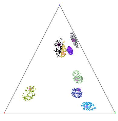
1. Introduction: Motivation and Background
1.1. Clustering Histograms in the Bag-of-Word Modeling Paradigm
A common task of information retrieval (IR) systems is to classify documents into categories. Given a training set of documents labeled with categories, one asks to classify new incoming documents. Text categorisation [1,2] proceeds by first defining a dictionary of words from a corpus. It then models each document by a word count yielding a word distribution histogram per document (see the University of California, Irvine, UCI, machine learning repository for such data-sets [3]). The importance of the words in the dictionary can be weighted by the term frequency-inverse document frequency [2] (tf-idf) that takes into account both the frequency of the words in a given document, but also of the frequency of the words in all documents: Namely, the tf-idf weight for a given word in a given document is the product of the frequency of that word in the document times the logarithm of the ratio of the number of documents divided by the document frequency of the word [2]. Defining a proper distance between histograms allows one to:
Classify a new on-line document: We first calculate its word distribution histogram signature and seek for the labeled document, which has the most similar histogram to deduce its category tag.
Find the initial set of categories: we cluster all document histograms and assign a category per cluster.
This text classification method based on the representation of the bag-of -words (BoWs) has also been instrumental in computer vision for efficient object categorization [4] and recognition in natural images [5]. This paradigm is called bag-of-features [6] (BoFs) in the general case. It first requires one to create a dictionary of “visual words” by quantizing keypoints (e.g., affine invariant descriptors of image patches) of the training database. Quantization is performed using the k-means [7–9] algorithm that partitions n data into k pairwise disjoint clusters C1,…, Ck, where each data element belongs to the closest cluster center (i.e., the cluster prototype). From a given initialization, batched k-means first assigns data points to their closest centers and then updates the cluster centers and reiterates this process until convergence is met to a local minimum (not necessarily the global minimum) after a provably finite number of steps. Csurka et al. [4] used the squared Euclidean distance for building the visual vocabulary. Depending on the chosen features, other distances have proven useful. For example, the symmetrized Kullback–Leibler (KL) divergence was shown to perform experimentally better than the Euclidean or squared Euclidean distances for a compressed histogram of gradient descriptors [10] (CHoGs), even if it is not a metric distance, since its fails to satisfy the triangular inequality. To summarize, k-means histogram clustering with respect to the symmetrized KL (called Jeffreys divergence J) can be used to quantize both visual words and document categories. Nowadays, the seminal bag-of-word method has been generalized fruitfully to various settings using the generic bag-of-X paradigm, like the bag-of-textons [6], the bag-of-readers [11], etc. Bag-of-X represents each data (e.g., document, image, etc.) as an histogram of codeword count indices. Furthermore, the semantic space [12] paradigm has been recently explored to overcome two drawbacks of the bag-of-X paradigms: the high-dimensionality of the histograms (number of bins) and difficult human interpretation of the codewords due to the lack of semantic information. In semantic space, modeling relies on semantic multinomials that are discrete frequency histograms; see [12].
In summary, clustering histograms with respect to symmetric distances (like the symmetrized KL divergence) is playing an increasing role. It turns out that the symmetrized KL divergence belongs to a 1-parameter family of divergences, called symmetrized α-divergences, or Jeffreys α-divergence [13].
1.2. Contributions
Since divergences D(p : q) are usually asymmetric distortion measures between two objects p and q, one has to often consider two kinds of centroids obtained by carrying the minimization process either on the left argument or on the right argument of the divergences; see [14]. In theory, it is enough to consider only one type of centroid, say the right centroid, since the left centroid with respect to a divergence D(p : q) is equivalent to the right centroid with respect to the mirror divergence D′(p : q) = D(q : p). In this paper, we consider mixed divergences [15] that allow one to handle in a unified way the arithmetic symmetrization of a given divergence D(p : q) with both the sided divergences: D(p : q) and its mirror divergence D′(p : q). The mixed α-divergence is the mixed divergence obtained for the α-divergence. We term α-clustering the clustering with respect to α-divergences and mixed α-clustering the clustering w.r.t. mixed α-divergences [16]. Our main contributions are to extend the celebrated batched k-means [7–9] algorithm to mixed divergences by associating two dual centroids per cluster and to generalize the probabilistically guaranteed good seeding of k-means++ [17] to mixed α-divergences. The mixed α-seedings provide guaranteed probabilistic clustering bounds by picking up seeds from the data and do not require explicitly computing of centroids. Therefore, it follows a fast clustering technique in practice, even when cluster centers are not available in closed form. We also consider clustering histograms by explicitly building the symmetrized α-centroids and end up with a variational k-means when the centroids are not available in closed-form, Finally, we investigate soft mixed α-clustering and discuss topics related to α-clustering. Note that clustering with respect to non-symmetrized α-divergences has been recently investigated independently in [18] and proven useful in several applications.
1.3. Outline of the Paper
The paper is organized as follows: Section 2 introduces the notion of mixed divergences, presents an extension of k-means to mixed divergences and recalls some properties of α-divergences. Section 3 describes the α-seeding techniques and reports a probabilistically-guaranteed bound on the clustering quality. Section 4 investigates the various sided/symmetrized/mixed calculations of the α-centroids. Section 5 presents the soft α-clustering with respect to α-mixed divergences. Finally, Section 6 summarises the contributions, discusses related topics and hints at further perspectives. The paper is followed by two appendices. Appendix B studies several properties of α-divergences that are used to derive the guaranteed probabilistic performance of the α-seeding. Appendix C proves that α-sided centroids are quasi-arithmetic means for the power generator functions.
2. Mixed Centroid-Based k-Means Clustering
2.1. Divergences, Centroids and k-Means
Consider a set of n histograms h1,…, hn, each with d bins, with all positive real-valued bins: , ∀1 ≤ i ≤ d, 1 ≤ j ≤ n. A histogram h is called a frequency histogram when its bins sums up to one: . Otherwise, it is called a positive histogram that can eventually be normalized to a frequency histogram:
The frequency histograms belong to the (d-1)-dimensional open probability simplex Δd:
That is, although frequency histograms have d bins, the constraint that those bin values should sum up to one yields d-1 degrees of freedom. In probability theory, the frequency or counting of histograms either model discrete multinomial probabilities or discrete positive measures (also called positive arrays [19]).
The celebrated k-means clustering [8,9] is one of the most famous clustering techniques that has been generalized in many ways [20,21]. In information geometry [22], a divergence D(p : q) is a smooth C3 differentiable dissimilarity measure that is not necessarily symmetric (D(p : q) ≠ D(q : p), hence the notation “:” instead of the classical “,” reserved for metric distances), but is non-negative and satisfies the separability property: D(p : q) = 0 iff p = q. More precisely, let , . Then, we require ∂iD(x : x) = ∂,iD(x : x) = 0 and −∂i∂,jD(x : y) positive definite for defining a divergence. For a distance function D(· : ·), we denote by the weighted average distance of x to a set a weighted histograms:
An important class of divergences on frequency histograms is the f-divergences [23–25] defined for a convex generator f (with f′(1) = f′(1) = 0 and f″(1) = 1):
Those divergences preserve information monotonicity [19] under any arbitrary transition probability (Markov morphisms). f-divergences can be extended to positive arrays [19].
The k-means algorithm on a set of weighted histograms can be tailored to any divergence as follows: First, we initialize the k cluster centers C = {c1,…, ck} (say, by picking up randomly arbitrary distinct seeds). Then, we iteratively repeat until convergence the following two steps:
Assignment: Assign each histogram hj to its closest cluster center:
This yields a partition of the histogram set , where Al denotes the set of histograms of the l-th cluster: .Center relocation: Update the cluster centers by taking their centroids:
Throughout this paper, centroid shall be understood in the broader sense of a barycenter when weights are non-uniform.
2.2. Mixed Divergences and Mixed k-Means Clustering
Since divergences are potentially asymmetric, we can define two-sided k-means or always consider a right-sided k-means, but then define another sided divergence D′(p : q) = D(q : p). We can also consider the symmetrized k-means with respect to the symmetrized divergence: S(p, q) = D(p : q) + D(q : p). Eventually, we may skew the symmetrization with a parameter λ ∈ [0, 1]: Sλ(p, q) = λD(p : q) + (1 − λ)D(q : p) (and consider other averaging schemes instead of the arithmetic mean).
In order to handle those sided and symmetrized k-means under the same framework, let us introduce the notion of mixed divergences [15] as follows:
Definition 1 (Mixed divergence).
for λ ∈ [0, 1].
A mixed divergence includes the sided divergences for λ ∈ {0, 1} and the symmetrized (arithmetic mean) divergence for .
We generalize k-means clustering to mixed k-means clustering [15] by considering two centers per cluster (for the special cases of λ = 0, 1, it is enough to consider only one). Algorithm 1 sketches the generic mixed k-means algorithm. Note that a simple initialization consists of choosing randomly the k distinct seeds from the dataset with li = ri.
Notice that the mixed k-means clustering is different from the k-means clustering with respect to the symmetrized divergences Sλ that considers only one centroid per cluster.
2.3. Sided, Symmetrized and Mixed α-Divergences
For α ≠ ±1, we define the family of α-divergences [26] on positive arrays [27] as:
with the limit cases D−1(p : q) = KL(p : q) and D1(p : q) = KL(q : p), where KL is the extended Kullback–Leibler divergence:
Divergence D0 is the squared Hellinger symmetric distance (scaled by a multiplicative factor of four) extended to positive arrays:
with the Hellinger distance:
Note that α-divergences are defined for the full range of α values: α ∈ ℝ. Observe that α-divergences of Equation (5) are homogeneous of degree one: Dα(λp : λq) = λDα(p : q) for λ > 0.
When histograms p and q are both frequency histograms, we have:
and the extended Kullback–Leibler divergence reduces to the traditional Kullback–Leibler divergence: .
The Kullback–Leibler divergence between frequency histograms and (α = ±1) is interpreted as the cross-entropy minus the Shannon entropy:
Often, denotes the true model (hidden by nature), and is the estimated model from observations. However, in information retrieval, both and play the same symmetrical role, and we prefer to deal with a symmetric divergence.
The Pearson and Neyman χ2 distances are obtained for α = −3 and α = 3, respectively:
The α-divergences belong to the class of Csiszár f-divergences with the following generator:
Remark 1. Historically, the α-divergences have been introduced by Chernoff [28,29] in the context of hypothesis testing. In Bayesian binary hypothesis testing, we are asked to decide whether an observation belongs to one class or the other class, based on prior w1 and w2 and class-conditional probabilities p1 and p2. The average expected error of the best decision maximum a posteriori (MAP) rule is called the probability of error, denoted by Pe. When prior probabilities are identical, we have. Let S(p, q) = ∫ min(p(x), q(x))dx denote the intersection similarity measure, with 0 < S ≤ 1 (generalizing the histogram intersection distance often used in computer vision [30]). S is bounded by the α-Chernoff affinity coefficient:
for all β ∈ [0, 1]. We can convert the affinity coefficient 0 < Cβ ≤ 1 into a divergence Dβ by simply taking Dβ = 1 − Cβ. Since the absolute value of divergences does not matter, we can rescale appropriately the divergence. One nice rescaling is by multiplying by. This lets coincide the parameterized divergence with the fundamental Kullback–Leibler divergence for the limit values β ∈ {0, 1}. Last, by choosing, it yields the well-known expression of the α-divergences.
Interestingly, the α-divergences can be interpreted as a generalized α-Kullback–Leibler divergence [26] with deformed logarithms.
Next, we introduce the mixed α-divergence of a histogram x to two histograms p and q as follows:
Definition 2 (Mixed α-divergence). The mixed α-divergence of a histogram x to two histograms p and q is defined by:
The α-Jeffreys symmetrized divergence is obtained for :
The skew symmetrized α-divergence is defined by:
2.4. Notations and Hard/Soft Clusterings
Throughout the paper, superscript index i denotes the histogram bin numbers and subscript index j the histogram numbers. Index l is used to iterate on the clusters. The left-sided, right-sided and symmetrized histogram positive and frequency α-centroids are denoted by lα, rα, sα and , respectively.
In this paper, we investigate the following kinds of clusterings for sets of histograms:
Hard clustering. Each histogram belongs to exactly one cluster:
k-means with respect to mixed divergences Mλ,α.
k-means with respect to symmetrized divergences Sλ,α.
Randomized seeding for mixed/symmetrized k-means by extending k-means++ with guaranteed probabilistic bounds for α-divergences.
Soft clustering. Each histogram belongs to all clusters according to some weight distribution: the soft mixed α-clustering.
3. Coupled k-Means++ α-Seeding
It is well-known that the Lloyd k-means clustering algorithm monotonically decreases the loss function and stops after a finite number of iterations into a local optimal. Optimizing globally the k-means loss is NP-hard [17] when d > 1 and k > 1. In practice, the performance of the k-means algorithm heavily relies on the initialization. A breakthrough was obtained by the k-means++ seeding [17], which guarantees in expectation a good starting partition. We extend this scheme to the coupled α-clustering. However, we point out that although k-means++ prove popular and are often used in practice with very good results; it has been recently pointed out that “worst case” configurations exist and even in small dimensions, on which the algorithm cannot beat significantly its expected approximability with a high probability [31]. Still, the expected approximability ratio, roughly in O(log(k)), is very good, as long as the number of clusters is not too large.
Algorithm 2 provides our adaptation of k-means++ seeding [15,17]. It works for all three of our sided/symmetrized and mixed clustering settings:
Pick λ = 1 for the left-sided centroid initialization,
Pick λ = 0 for the right-sided centroid initialization (a left-sided initialization for −α),
with arbitrary λ, for the λ-Jα (skew Jeffreys) centroids or mixed λ centroids. Indeed, the initialization is the same (see the MAS procedure in Algorithm 2).
Our proof follows and generalizes the proof described for the case of mixed Bregman seeding [15] (Lemma 2). In fact, our proof is more precise, as it quantifies the expected potential with respect to the optimum only, whereas in [15], the optimal potential is averaged with a dual optimal potential, which depends on the optimal centers, but may be larger than the optimum sought.
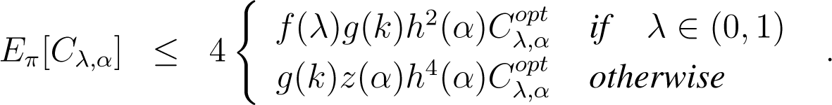
Theorem 1. Let Cλ,α denote for short the cost function related to the clustering type chosen (left-, right-, skew Jeffreys or mixed) in MASand denote the optimal related clustering in k clusters, for λ ∈ [0, 1] and α ∈ (−1, 1). Then, on average, with respect to distribution (14), the initial clustering of MAS satisfies:

Here , g(k) = 2(2 + log k), , ; the min is defined on strictly positive coordinates, and π denotes distribution of Algorithm 2.
Remark 2. The bound is particularly good when λ is close to 1/2, and in particular for the α-Jeffreys clustering, as in these cases, the only additional penalty compared to the Euclidean case [17] is h2(α), a penalty that relies on an optimal triangle inequality for α-divergences that we provide in Lemma 8 below.
Remark 3. This guaranteed initialization is particularly useful for α-Jeffreys clustering, as there is no closed form solution for the centroids (except when α = ±1, see [32]).
Algorithm 3 presents the general hard mixed k-means clustering, which can be adapted also to left- (λ = 1) and right- (λ = 0) α-clustering.
For skew Jeffreys centers, since the centroids are not available in closed form [32], we adopt a variational approach of k-means by updating iteratively the centroid in each cluster (thus improving the overall loss function without computing the optimal centroids that would eventually require infinitely many iterations).
4. Sided, Symmetrized and Mixed α-Centroids
The k-means clustering requires assigning data elements to their closest cluster center and then updating those cluster centers by taking their centroids. This section investigates the centroid computations for the sided, symmetrized and mixed α-divergences.
Note that the mixed α-seeding presented in Section 3 does not require computing centroids and, yet, guarantees probabilistically a good clustering partition.
Since mixed α-divergences are f-divergences, we start with the generic f-centroids.
4.1. Csiszár f-Centroids
The centroids induced by f-divergences of a set of positive measures (that relaxes the normalisation constraint) have been studied by Ben-Tal et al. [33]. Those entropic centroids are shown to be unique, since f-divergences are convex statistical distances in both arguments. Let Ef denote the energy to minimize when considering f-divergences:
When the domain is the open probability simplex , we get a constrained optimisation problem to solve. We transform this constrained minimisation problem (i.e., x ∈ Δd) into an equivalent unconstrained minimisation problem by using the Lagrange multiplier, γ:
Taking the derivatives according to xi, we get:
We now consider this equation for α-divergences and symmetrized α-divergences, both f-divergences.
4.2. Sided Positive and Frequency α-Centroids
The positive sided α-centroids for a set of weighted histograms were reported in [34] using the representation Bregman divergence. We summarise the results in the following theorem:
Theorem 2 (Sided positive α-centroids [34]). The left-sided lα and right-sided rα positive weighted α-centroid coordinates of a set of n positive histograms h1,…, hn are weighted α-means:
with
Furthermore, the frequency-sided α-centroids are simply the normalized-sided α-centroids.
Theorem 3 (Sided frequency α-centroids [16]). The coordinates of the sided frequency α-centroids of a set of n weighted frequency histograms are the normalised weighted α-means.
Table 1 summarizes the results concerning the sided positive and frequency α-centroids.
4.3. Mixed α-Centroids
The mixed α-centroids for a set of n weighted histograms is defined as the minimizer of:
We state the theorem generalizing [15]:
Theorem 4. The two mixed α-centroids are the left-sided and right-sided α-centroids.
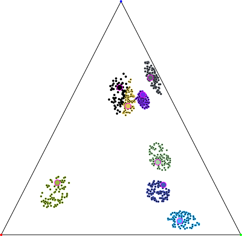
Figure 1 depicts some clustering result with our α-clustering software. We remark that the clusters found are all approximately subclusters of the “distinct” clusters that appear on the figure. When those distinct clusters are actually the optimal clusters—which is likely to be the case when they are separated by large minimal distance to other clusters—this is clearly a desirable qualitative property as long as the number of experimental clusters is not too large compared to the number of optimal clusters. We remark also that in the experiment displayed, there is no closed form solution for the cluster centers.
4.4. Symmetrized Jeffreys-Type α-Centroids
The Kullback–Leibler divergence can be symmetrized in various ways: Jeffreys divergence, Jensen–Shannon divergence and Chernoff information, just to mention a few. Here, we consider the following symmetrization of α-divergences extending Jeffreys J-divergence:
For α = ±1, we get half of Jeffreys divergence:
In particular, when p and q are frequency histograms, we have for α ≠ ±1:
where a symmetric Heinz mean [35,36]:
Heinz means interpolate the arithmetic and geometric means and satisfies the inequality:
(Another interesting property of Heinz means is the integral representation of the logarithmic mean: . This allows one to prove easily that .)
The Jα-divergence is a Csiszár f-divergence [24,25].
Observe that it is enough to consider α ∈ [0, ∞) and that the symmetrized α-divergence for positive and frequency histograms coincide only for α = ±1.
For α = ±1, Sα(p, q) tends to the Jeffreys divergence:
The Jeffreys divergence writes mathematically the same for frequency histograms:
We state the results reported in [32]:
Theorem 5 (Jeffreys positive centroid [32]). The Jeffreys positive centroid c = (c1,…, cd) of a set {h1,…, hn} of n weighted positive histograms with d bins can be calculated component-wise exactly using the Lambert W analytic function:
where denotes the coordinate-wise arithmetic weighted means and the coordinate-wise geometric weighted means.
The Lambert analytic function W [37] (positive branch) is defined by W (x)eW(x) = x for x ≥ 0.
Theorem 6 (Jeffreys frequency centroid [32]). Let denote the Jeffreys frequency centroid and the normalised Jeffreys positive centroid. Then, the approximation factor is such that (with wc ≤ 1)
Therefore, we shall consider α ≠ ±1 in the remainder.
We state the following lemma generalizing the former results in [38] that were tailored to the symmetrized Kullback–Leibler divergence or the symmetrized Bregman divergence [14]:
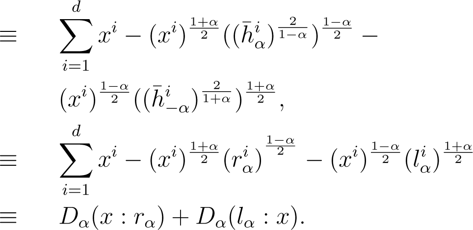
Lemma 1 (Reduction property). The symmetrized Jα-centroid of a set of n weighted histograms amount to computing the symmetrized α-centroid for the weighted α-mean and −α-mean:
Proof. It follows that the minimization problem reduces to the following minimization:
This is equivalent to minimizing:

Note that α = ±1, the lemma states that the minimization problem is equivalent to minimizing KL(a : x) + KL(x : g) with respect to x, where a = l1 and g = r1 denote the arithmetic and geometric means, respectively. □
The lemma states that the optimization problem with n weighted histograms is equivalent to the optimization with only two equally weighted histograms.
The positive symmetrized α-centroid is equivalent to computing a representation symmetrized Bregman centroid [14,34].
The frequency symmetrized α-centroid asks to minimize the following problem:
Instead of seeking for in the probability simplex, we can optimize on the unconstrained domain ℝd−1 by using a reparameterization. Indeed, frequency histograms belong to the exponential families [39] (multinomials).
Exponential families also include many other continuous distributions, like the Gaussian, Beta or Dirichlet distributions. It turns out the α-divergences can be computed in closed-form for members of the same exponential family:
Lemma 2. The α-divergence for distributions belonging to the same exponential families amounts to computing a divergence on the corresponding natural parameters:
where is a skewed Jensen divergence defined for the log-normaliser F of the family.
The proof follows from the fact that ; see [40].
First, we convert a frequency histogram to its natural parameter θ with ; see [39].
The log-normaliser is a non-separable convex function . To convert back a multinomial to a frequency histogram with d bins, we first set and then retrieve the other bin values as .
The centroids with respect to skewed Jensen divergences has been investigated in [13,40].
Remark 4. Note that for the special case of α = 0 (squared Hellinger centroid), the sided and symmetrized centroids coincide. In that case, the coordinates of the squared Hellinger centroid are:
Remark 5. The symmetrized positive α-centroids can be solved in special cases (α = ±3, α = ±1 corresponding to the symmetrized χ2 and Jeffreys positive centroids). For frequency centroids, when dealing with binary histograms (d = 2), we have only one degree of freedom and can solve the binary frequency centroids. Binary histograms (and mixtures thereof) are used in computer vision and pattern recognition [41].
Remark 6. Since α-divergences are Csiszár f-divergences and f-divergences can always be symmetrized by taking generator, we deduce that symmetrized α-divergences Sα are f-divergences for the generator:
Hence, Sα divergences are convex in both arguments, and the sα centroids are unique.
5. Soft Mixed α-Clustering
Algorithm 4 reports the general clustering with soft membership, which can be adapted to left (λinit = 1), right (λinit = 0) or mixed clustering. We have not considered a weighted histogram set in order not load the notations and because the extension is straightforward.
Again, for skew Jeffreys centers, we shall adopt a variational approach. Notice that the soft clustering approach learns all parameters, including λ (if not constrained to zero or one) and α ∈ ℝ. This is not the case for Matsuyama’s α-expectation maximization (EM) algorithm [42] in which α is fixed beforehand (and, thus, not learned).
Assuming we model the prior for histograms by:
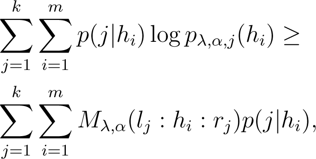
the negative log-likelihood involves the α-depending quantity:

because of the concavity of the logarithm function. Therefore, the maximization step for α involves finding:
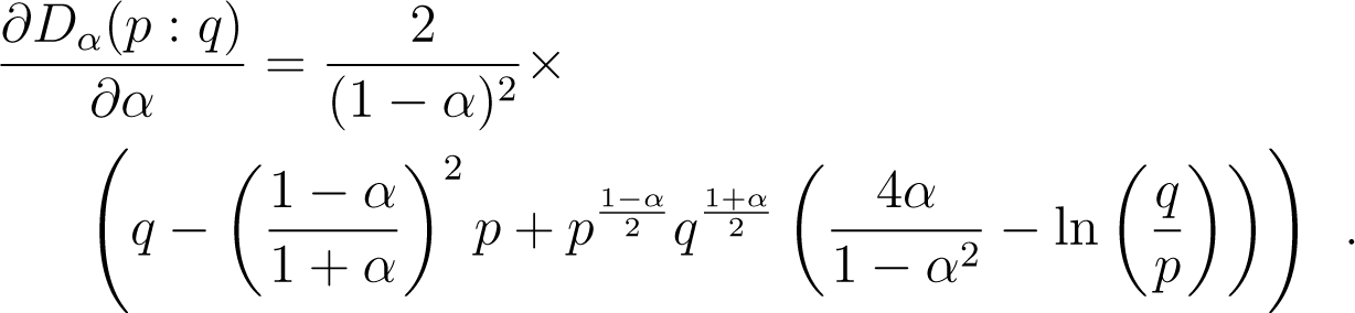
No closed-form solution are known, so we compute the gradient update in Algorithm 4 with:

The update in λ is easier as:
Maximizing the likelihood in λ would imply choosing λ ∈ {0, 1} (a hard choice for left/right centers), yet we prefer the soft update for the parameter, like for α.
6. Conclusions
The family of α-divergences plays a fundamental role in information geometry: These statistical distortion measures are the canonical divergences of dual spaces on probability distribution manifolds with constant curvature and the canonical divergences of dually flat manifolds for positive distribution manifolds [19].
In this work, we have presented three techniques for clustering (positive or frequency) histograms using k-means:
- (1)
Sided left or right α-centroid k-means,
- (2)
Symmetrized Jeffreys-type α-centroid (variational) k-means, and
- (3)
Coupled k-means with respect to mixed α-divergences relying on dual α-centroids.
Sided and mixed dual centroids are always available in closed-forms and are therefore highly attractive from the standpoint of implementation. Symmetrized Jeffreys centroids are in general not available in closed-form and require one to implement a variational k-means by updating incrementally the cluster centroids in order to monotonically decrease the k-means loss function. From the clustering standpoint, this appears not to be a problem when guaranteed expected approximations to the optimal clustering are enough.
Indeed, we also presented and analyzed an extension of k-means++ [17] for seeding those k-means algorithms. The mixed α-seeding initializations do not require one to calculate centroids and behaves like a discrete k-means by picking up the seeds among the data. We reported guaranteed probabilistic clustering bounds. Thus, it yields a fast hard/soft data partitioning technique with respect to mixed or symmetrized α-divergences. Recently, the advantage of clustering using α-divergences by tuning α in applications has been demonstrated in [18]. We thus expect the computationally fast mixed α-seeding with guaranteed performance to be useful in a growing number of applications.
Acknowledgments
NICTA is funded by the Australian Government as represented by the Department of Broadband, Communication and the Digital Economy and the Australian Research Council through the ICT Centre of Excellence program.
Author Contributions
All authors contributed equally to the design of the research. The research was carried out by all authors. Frank Nielsen and Richard Nock wrote the paper. Frank Nielsen implemented the algorithms and performed experiments. All authors have read and approved the final manuscript.
Conflicts of Interest
The authors declare no conflict of interests.
Appendix
A. Proof Sketch of Theorem 1
We give here the key results allowing one to obtain the proof of the Theorem, following the proof scheme of [15]. In order not to load the notations, weights are considered uniform. The extension to non-uniform weights is immediate as it boils down to duplicate histograms in the histogram set and does not change the approximation result.
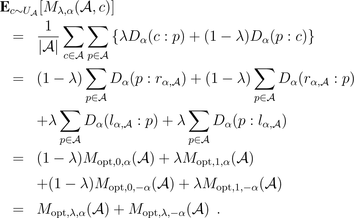
Let be an arbitrary cluster of Copt. Let us define and as the uniform and biased distributions conditioned to . The key to the proof is to relate the expected potential of under and to its contribution to the optimal potential.
Lemma 3. Let be an arbitrary cluster of Copt. Then:

where is the uniform distribution over .
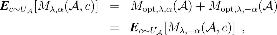
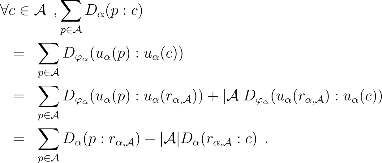
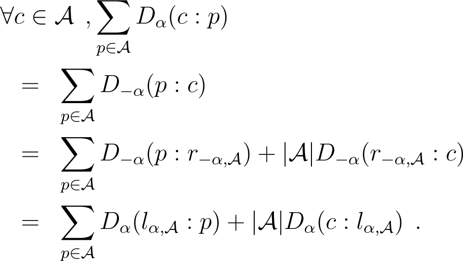
Proof. α-coordinates have the property that for any subset , . Hence, we have:

Because Dα(p : q) = D−α(q : p) and lα = r−α, we obtain:

It comes now from (33) and (34) that:

This gives the left-hand side equality of the Lemma. The right-hand side follows from the fact that . □
Instead of , we want a term depending solely on as it is the “true” optimum. We now give two lemmata that shall be useful in obtaining this upper bound. The first is of independent interest, as it shows that any α-divergence is a scaled, squared Hellinger distance between geometric means of points.
Lemma 4. For any p, q and α ≠ 1, there exists r ∈ [p, q], such that (1 − α)2Dα(p : q) = D0(p1−αrα : q1−αrα).
Proof. By the definition of Bregman divergences, for any x, y, there exists some z ∈ [x, y], such that:

and since uα is continuous and strictly increasing, for any p, q, there exists some r ∈ [p, q], such that:

Lemma 5. Let discrete random variable x take non-negative values x1, x2,…, xm with uniform probabilities. Then, for any β > −1, we have var(x1+β/uβ) ≤ var(x), with.
Proof. First, ∀β > −1, remark that for any x, function f(x) = x(uβ − xβ) is increasing for x ≤ u/(1 + β)β. Hence, assuming that the xis are put in non-increasing order without loss of generality, we have f(xi) ≥ f(xj), and so, , ∀i ≥ j, as long as xi ≤ u/(1 + β)β. Choosing u = x1(1 + β)β yields, after reordering and putting the exponent, . Hence:

Dividing by u2β the leftmost and rightmost terms and using the fact that var(λx) = λ2var(x) yields the statement of the Lemma. □
We are now ready to upper bound as a function of .
Lemma 6. For any cluster of Copt,

where z(α), f(λ) and h(α) are defined in Theorem 1.
Proof. The case λ ≠ 0, 1 is fast, as we have by definition:

Suppose now that λ = 0 and α ≥ 0. Because , what we wish to do is upper bound as a function of . We use Lemmatas 4 and 5 in the following derivations, using r(p) to refer to the r in Lemma 4, assuming α ≥ 0. We also note as the variance, under the uniform distribution over , of discrete random variable f(p), for . We have:

We have used the expression of left centroid to simplify the expressions. Now, picking , β = 2α/(1 − α) and in Lemma 5 yields:

Plugging this in (36) yields:


Here, (38) follows the path backwards of derivations that lead to (36). The cases λ = 1 or α < 0 are obtained using the same chains of derivations and achieve the proof of Lemma 6. □
Lemma 6 can be directly used to refine the bound of Lemma 3 in the uniform distribution. We give the Lemma for the biased distribution, directly integrating the refinement of the bound.
Lemma 7. Let be an arbitrary cluster of Copt and C an arbitrary clustering. If we add a random couple (c, c) to C, chosen from with π as in Algorithm 2, then:

where f(λ) and h(α) are defined in Theorem 1.
Proof. The proof essentially follows the proof of Lemma 3 in [15]. To complete it, we need a triangle inequality involving α-divergences. We give it here.
Lemma 8. For any p, q, r and α, we have:

(where the min is over strictly positive values)
Remark: take α = 0; we find the triangle inequality for the squared Hellinger distance.
Proof. Using the proof of Lemma 2 in [15] for Bregman divergence , we get:
where:
Taking x = uα(p), y = uα(q), z = uα(r) yields and the statement of Lemma 8. □
The rest of the proof of Lemma 7 follows the proof of Lemma 3 in [15]. □
We get all of the ingredients to our proof, and there remains to use Lemma 4 in [15] to achieve the proof of Theorem 1.
B. Properties of α-Divergences
For positive arrays p and q, the α-divergence Dα(p : q) can be defined as an equivalent representational Bregman divergence [19,34] over the (uα, υα)-structure [43] with:
where we assume that α ≠ ±1. Otherwise, for α = ±1, we compute Dα(p : q) by taking the sided Kullback–Leibler divergence extended to positive arrays.
In the proof of Theorem 1, we have used two properties of α-divergences of independent interest:
any α-divergence can be explained as a scaled squared Hellinger distance between geometric means of its arguments and a point that belong to their segment (Lemma 4);
any α-divergence satisfies a generalized triangle inequality (Lemma 8). Notice that this Lemma is optimal in the sense that for α = 0, it is possible to recover the triangle inequality of the Hellinger distance.
The following lemma shows how to bound the mixed divergence as a function of an α-divergence.
Lemma 9. For any positive arrays l, h, r and α ≠ ±1, define, with and aη with. Then, we have:

Proof. For all index i, we have:


The arithmetic-geometric-harmonic (AGH) inequality implies:

It follows that (48) yields:


out of which we get the statement of the Lemma. □
C. Sided α-Centroids
For the sake of completeness, we prove the following theorem:
Theorem 7 (Sided positive α-centroids [34]). The left-sided lα and right-sided rα positive weighted α-centroid coordinates of a set of n positive histograms h1,…, hn are weighted α-means:
with:
Proof. We distinguish three cases: α ≠ ±1, α = −1 and α = 1.
First, consider the general case α ≠ ±1. We have to minimize:

Removing all additive terms independent of xi and the overall constant multiplicative factor , we get the following equivalent minimisation problem:
where denote the following aggregation term:
Setting coordinate-wise the derivative to zero of Equation (51), we get:
Thus, we find that the coordinates of the right-sided α-centroids are:
We recognise the expression of a quasi-arithmetic mean for the strictly monotonous generator fα(x):
with:
Therefore, we conclude that the coordinates of the positive α-centroid are the weighted α-means of the histogram coordinates (for α ≠ ±1). Quasi-arithmetic means are also called in the literature quasi-linear means or f-means.
When α = −1, we search for the right-sided extended Kullback–Leibler divergence centroid by minimising:
It is equivalent to minimizing:
where a denotes the arithmetic mean. Solving coordinate-wise, .
When α = 1, the right-sided reverse extended KL centroid is a left-sided extended KL centroid. The minimisation problem is:
Since ∑jwj = 1, we solve coordinate-wise and find log x = ∑jwj log hj. That is, is the geometric mean:
Both the arithmetic mean and the geometric mean are power means in the limit case (and hence quasi-arithmetic means). Thus,
with:
References
- Baker, L.D.; McCallum, A.K. Distributional clustering of words for text classification, Proceedings of the 21st Annual International ACM SIGIR Conference on Research and Development in Information Retrieval, Melbourne, Australia, 24–28 August 1998; ACM: New York, NY, USA, 1998; pp. 96–103.
- Bigi, B. Using Kullback–Leibler distance for text categorization, Proceedings of the 25th European conference on IR research (ECIR), Pisa, Italy, 14–16 April 2003; Springer-Verlag: Berlin/Heidelberg, Germany, 2003; ECIR’03. pp. 305–319.
- Bag of Words Data Set, Available online: http://archive.ics.uci.edu/ml/datasets/Bag+of+Words (accessed 17 June 2014).
- Csurka, G.; Bray, C.; Dance, C.; Fan, L. Visual Categorization with Bags of Keypoints, Workshop on Statistical Learning in Computer Vision (ECCV); Xerox Research Centre Europe: Meylan, France, 2004; pp. 1–22.
- Jégou, H.; Douze, M.; Schmid, C. Improving Bag-of-Features for Large Scale Image Search. Int. J. Comput. Vis 2010, 87, 316–336. [Google Scholar]
- Yu, Z.; Li, A.; Au, O.; Xu, C. Bag of textons for image segmentation via soft clustering and convex shift, Proceedings of 2012 IEEE Conference on Computer Vision and Pattern Recognition (CVPR), Providence, RI, USA, 16–21 June 2012; pp. 781–788.
- Steinhaus, H. Sur la division des corp matériels en parties. Bull. Acad. Polon. Sci 1956, 1, 801–804. (in French). [Google Scholar]
- Lloyd, S.P. Least Squares Quantization in PCM; Technical Report RR-5497; Bell Laboratories: Murray Hill, NJ, USA, 1957. [Google Scholar]
- Lloyd, S.P. Least squares quantization in PCM. IEEE Trans. Inf. Theory 1982, 28, 129–137. [Google Scholar]
- Chandrasekhar, V.; Takacs, G.; Chen, D.M.; Tsai, S.S.; Reznik, Y.A.; Grzeszczuk, R.; Girod, B. Compressed histogram of gradients: A low-bitrate descriptor. Int. J. Comput. Vis 2012, 96, 384–399. [Google Scholar]
- Nock, R.; Nielsen, F.; Briys, E. Non-linear book manifolds: Learning from associations the dynamic geometry of digital libraries, Proceedings of the 13th ACM/IEEE-CS Joint Conference on Digital Libraries, New York, NY, USA; 2013; pp. 313–322.
- Kwitt, R.; Vasconcelos, N.; Rasiwasia, N.; Uhl, A.; Davis, B.C.; Häfner, M.; Wrba, F. Endoscopic image analysis in semantic space. Med. Image Anal 2012, 16, 1415–1422. [Google Scholar]
- Nielsen, F. A family of statistical symmetric divergences based on Jensen’s inequality 2010, arXiv, 1009.4004.
- Nielsen, F.; Nock, R. Sided and symmetrized Bregman centroids. IEEE Trans. Inf. Theory 2009, 55, 2882–2904. [Google Scholar]
- Nock, R.; Luosto, P.; Kivinen, J. Mixed Bregman clustering with approximation guarantees, Proceedings of the European Conference on Machine Learning and Knowledge Discovery in Databases, Antwerp, Belgium, 15–19 September 2008; Springer-Verlag: Berlin/Heidelberg, Germany, 2008; pp. 154–169.
- Amari, S. Integration of Stochastic Models by Minimizing α-Divergence. Neural Comput 2007, 19, 2780–2796. [Google Scholar]
- Arthur, D.; Vassilvitskii, S. k-means++: The advantages of careful seeding, Proceedings of the Eighteenth Annual ACM-SIAM Symposium on Discrete Algorithms (SODA), New Orleans, LA, USA, 7–9 January 2007; Society for Industrial and Applied Mathematics: Philadelphia, PA, USA, 2007; pp. 1027–1035.
- Olszewski, D.; Ster, B. Asymmetric clustering using the alpha-beta divergence. Pattern Recognit 2014, 47, 2031–2041. [Google Scholar]
- Amari, S. Alpha-divergence is unique, belonging to both f-divergence and Bregman divergence classes. IEEE Trans. Inf. Theory 2009, 55, 4925–4931. [Google Scholar]
- Banerjee, A.; Merugu, S.; Dhillon, I.S.; Ghosh, J. Clustering with Bregman divergences. J. Mach. Learn. Res 2005, 6, 1705–1749. [Google Scholar]
- Teboulle, M. A unified continuous optimization framework for center-based clustering methods. J. Mach. Learn. Res 2007, 8, 65–102. [Google Scholar]
- Amari, S.; Nagaoka, H. Methods of Information Geometry; Oxford University Press: Oxford, UK, 2000. [Google Scholar]
- Morimoto, T. Markov Processes and the H-theorem. J. Phys. Soc. Jpn 1963, 18, 328–331. [Google Scholar]
- Ali, S.M.; Silvey, S.D. A general class of coefficients of divergence of one distribution from another. J. R. Stat. Soc. Ser. B 1966, 28, 131–142. [Google Scholar]
- Csiszár, I. Information-type measures of difference of probability distributions and indirect observation. Studi. Sci. Math. Hung 1967, 2, 229–318. [Google Scholar]
- Cichocki, A.; Cruces, S.; Amari, S. Generalized alpha-beta divergences and their application to robust nonnegative matrix factorization. Entropy 2011, 13, 134–170. [Google Scholar]
- Zhu, H.; Rohwer, R. Measurements of generalisation based on information geometry. In Mathematics of Neural Networks; Operations Research/Computer Science Interfaces Series; Ellacott, S., Mason, J., Anderson, I., Eds.; Springer: New York, NY, USA, 1997; Volume 8, pp. 394–398. [Google Scholar]
- Chernoff, H. A measure of asymptotic efficiency for tests of a hypothesis based on the sum of observations. Ann. Math. Stat 1952, 23, 493–507. [Google Scholar]
- Nielsen, F. An information-geometric characterization of Chernoff information. IEEE Signal Process. Lett 2013, 20, 269–272. [Google Scholar]
- Wu, J.; Rehg, J. Beyond the euclidean distance: creating effective visual codebooks using the histogram intersection kernel, Proceedings of 2009 IEEE 12th International Conference on Computer Vision, Kyoto, Japan, 29 September–2 October 2009; pp. 630–637.
- Bhattacharya, A.; Jaiswal, R.; Ailon, N. A tight lower bound instance for k-means++ in constant dimension. In Theory and Applications of Models of Computation; Lecture Notes in Computer Science; Gopal, T., Agrawal, M., Li, A., Cooper, S., Eds.; Springer International Publishing: New York, NY, USA, 2014; Volume 8402, pp. 7–22. [Google Scholar]
- Nielsen, F. Jeffreys centroids: A closed-form expression for positive histograms and a guaranteed tight approximation for frequency histograms. IEEE Signal Process. Lett 2013, 20, 657–660. [Google Scholar]
- Ben-Tal, A.; Charnes, A.; Teboulle, M. Entropic means. J. Math. Anal. Appl 1989, 139, 537–551. [Google Scholar]
- Nielsen, F.; Nock, R. The dual Voronoi diagrams with respect to representational Bregman divergences, Proceedings of International Symposium on Voronoi Diagrams (ISVD), Copenhagen, Denmark, 23–26 June 2009; pp. 71–78.
- Heinz, E. Beiträge zur Störungstheorie der Spektralzerlegung. Math. Anna 1951, 123, 415–438. (in German). [Google Scholar]
- Besenyei, A. On the invariance equation for Heinz means. Math. Inequal. Appl 2012, 15, 973–979. [Google Scholar]
- Barry, D.A.; Culligan-Hensley, P.J.; Barry, S.J. Real values of the W -function. ACM Trans. Math. Softw 1995, 21, 161–171. [Google Scholar]
- Veldhuis, R.N.J. The centroid of the symmetrical Kullback–Leibler distance. IEEE Signal Process. Lett 2002, 9, 96–99. [Google Scholar]
- Nielsen, F.; Garcia, V. Statistical exponential families: A digest with flash cards, 2009. arXiv.org: 0911.4863.
- Nielsen, F.; Boltz, S. The Burbea-Rao and Bhattacharyya centroids. IEEE Trans. Inf. Theory 2011, 57, 5455–5466. [Google Scholar]
- Romberg, S.; Lienhart, R. Bundle min-hashing for logo recognition, Proceedings of the 3rd ACM Conference on International Conference on Multimedia Retrieval, Dallas, TX, USA, 16–19 April 2013; ACM: New York, NY, USA, 2013; pp. 113–120.
- Matsuyama, Y. The alpha-EM algorithm: Surrogate likelihood maximization using alpha-logarithmic information measures. IEEE Trans. Inf. Theory 2003, 49, 692–706. [Google Scholar]
- Amari, S.I. New developments of information geometry (26): Information geometry of convex programming and game theory. In Mathematical Sciences (suurikagaku); Number 605; The Science Company: Denver, CO, USA, 2013; pp. 65–74. (In Japanese) [Google Scholar]


| Positive centroid | Frequency centroid | |
|---|---|---|
 | ||
 |
 |
 |
 |
© 2014 by the authors; licensee MDPI, Basel, Switzerland This article is an open access article distributed under the terms and conditions of the Creative Commons Attribution license (http://creativecommons.org/licenses/by/3.0/).
Share and Cite
Nielsen, F.; Nock, R.; Amari, S.-i. On Clustering Histograms with k-Means by Using Mixed α-Divergences. Entropy 2014, 16, 3273-3301. https://doi.org/10.3390/e16063273
Nielsen F, Nock R, Amari S-i. On Clustering Histograms with k-Means by Using Mixed α-Divergences. Entropy. 2014; 16(6):3273-3301. https://doi.org/10.3390/e16063273
Chicago/Turabian StyleNielsen, Frank, Richard Nock, and Shun-ichi Amari. 2014. "On Clustering Histograms with k-Means by Using Mixed α-Divergences" Entropy 16, no. 6: 3273-3301. https://doi.org/10.3390/e16063273