A Maximum Entropy Method for a Robust Portfolio Problem

Abstract

We propose a continuous maximum entropy method to investigate the robust optimal portfolio selection problem for the market with transaction costs and dividends. This robust model aims to maximize the worst-case portfolio return in the case that all of asset returns lie within some prescribed intervals. A numerical optimal solution to the problem is obtained by using a continuous maximum entropy method. Furthermore, some numerical experiments indicate that the robust model in this paper can result in better portfolio performance than a classical mean-variance model.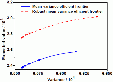

1. Introduction

Since Markowitz’s pioneering work [1,2], the mean-variance framework has become the foundation for modern finance theory. The concept of mean-variance analysis has been instrumental in many areas such as asset allocation and risk management during the past decades. Konno et al. [3] employed absolute deviation as a measure of risk which will lead to much less computation compared with those of mean-variance models. Young [4] formulated a min-max portfolio problem for maximizing the minimum return on the basis of historical returns data. Steinbach [5] provided an extensive overview of the mean-risk framework. Wu et al. [6] discussed a robust portfolio problem for the market with or without short sale restriction.

Although the mean-variance framework is still widely accepted and used, there are several challenges that are needed to be overcome. One of the major challenges is that optimal portfolios are sensitive to the estimation errors of mean and variance. Best and Grauer [7] analyzed the effect of changes in mean returns on the mean-variance efficient frontier and compositions of optimal portfolios. Broadie [8] investigated the impact of errors in parameter estimates on the actual frontiers, which were obtained by applying the true parameters to the portfolio weights derived from their estimated parameters. Both of these studies show that different input estimates to the mean-variance model can result in large variations in the composition of efficient portfolios.

In order to deal with the sensitivity of optimal portfolio to input data, many attempts have been made to develop new techniques such as optimization and parameter estimation. One of the techniques is a Bayesian approach to create stable expected returns. Black and Litterman [9] established a balance between the expected return and investor’s risk tolerance specified by a ranking of confidence. Another technique is the robust optimization which was first proposed by Soyster [10]. This approach is mainly to protect the decision-maker against parameter ambiguity. Most recently, many scholars considered the estimation errors of parameter by robust optimization. (see Goldfarb and Iyengar [11], Ceria and Stubbs [12], Ben-tal and Nemirovski [13]).

This paper proposes a continuous maximum entropy method to investigate the robust optimal portfolio selection problem for the market with transaction costs and dividends. Our focus will be on the following three cases. Firstly, all of the asset expected returns lie within some specified intervals which can be estimated by their historical return rates. This means that the errors in estimates of expected returns are considered by investors. It should be pointed out that our model only concerns this error, which is the major factor of estimation risk in the mean-variance framework. Secondly, we consider more complicated market situations than those in [6], in which they did not take into account transaction costs and dividends. As a matter of fact, it is an important issue in reality for portfolio managers to choose investment strategies (see Mansini and Speranza [14], Best and Hlouskova [15], Lobo et al. [16], Bertsimas and Lo [17]). Lastly, we apply a continuous maximum entropy method to solve a robust portfolio model. The discrete maximum entropy algorithm in [6] can not be applied to the present problem, because the objective function is not differentiable when transaction costs and dividends are considered.

The paper proceeds as follows: In Section 2, the robust portfolio model considering the market with transaction costs and dividends is discussed. Section 3 provides a numerical solution to the problem by using the maximum entropy method. Section 4 presents some numerical experiments with our model. Finally, concluding remarks and suggestions for future work are given in Section 5.

2. Problem Statement

Our focus here is to introduce the formulation of robust portfolio problem in a market with transaction costs and dividends. Therefore, we start with some notations and assumptions.

2.1. Notations and Assumptions

Assume that an investor allocates his initial wealth to n risky assets in a market with transaction costs and dividends, in which transaction costs include capital income tax and basic income tax. Let t_g be the tax rate of marginal capital income. t₀ is the tax rate of marginal basic income. t_f represents the commission rate of transaction. t_s is the stamp tax rate of transaction. The rate of dividends on asset i is specified by d_i. Let ${\tilde{r}}_i$ be the return rate of asset i, which is a random variable. Let r_i denote the mathematical expectation of the random variable of ${\tilde{r}}_i$. σ_ij is the covariance between the random variables ${\tilde{r}}_i$ and ${\tilde{r}}_j$. (σ_ij)_n×n is the matrix of asset volatilities, which can be used to measure the portfolio risk. Let $x_i^0$ and x_i be the proportion invested in asset i of initial portfolio and optimal portfolio respectively. The expected return and risk of a portfolio are respectively given by ${\displaystyle {\sum }_{i=1}^n{r}_i{x}_i}$ and ${\displaystyle {\sum }_{i=1}^n{\displaystyle {\sum }_{j=1}^n{\sigma }_{ij}{x}_i{x}_j}}$.

Next, we give the following assumptions:

Assumption 1. The covariance matrix (σ_ij)_n×n is strictly positively definite.

Assumption 2. The expected return for asset i is unknown-but-bounded. Instead of defining a box from an uncertain set, we consider that the expected return r_i is located in a known interval. That is, r_i ∈ (a_i, b_i), where a_i > 0, b_i > 0. They can be obtained by simulating from a probability model for future returns.

Assumption 3. The market considered in this paper includes transaction costs and dividends. The transaction cost is the V type function of the volume of transaction. The capital income tax contains the commission c₁(x) and stamp tax c₂(x). They are given by

$$c_1(x)={\displaystyle \sum _{i=1}^n{t}_f}\left|x_i-x_i^0\right|,c_2(x)={\displaystyle \sum _{i=1}^n{t}_s\left|x_i-x_i^0\right|}.$$

To make things easier, it is useful to define the following concepts. The net return is the total returns of expected return and dividends after paying the basic income tax and capital income tax. The pre-tax profit represents the total returns of expected return and dividends excluding the commission and stamp tax. The after-tax profit is the value of pre-tax profit after paying the capital income tax.

2.2. Robust Model

On the basis of the above notations and assumptions, we are now ready to formulate the robust portfolio model in the market with transaction costs and dividends.

Generally speaking, the stamp tax can be eliminated as a pre-tax expense in the period. However, the commission can not be ruled out since it is considered as investment cost. Therefore, the total pre-tax profit of a portfolio can be expressed by

$${\displaystyle \sum _{i=1}^n(r_i+d_i)x_i-c_1(x)-c_2(x)}.$$

Hence, the after-tax profit of a portfolio can be obtained by the following expression:

$${\displaystyle \sum _{i=1}^n(1-t_g)[(r_i+d_i)x_i-c_2(x)]-c_1(x)}.$$

Substituting expressions c₁(x) and c₂(x) into the above expression, it yields

$${\displaystyle \sum _{i=1}^n[(1-t_g)r_i+(1-t_0)d_i]x_i-{\displaystyle \sum _{i=1}^n[(1-t_g)t_s+t_f]|x_i-x_i^0|}.}$$

Define

$$R_i=(1-t_g)r_i+(1-t_0)d_i$$

and

$$k=(1-t_g)t_s+t_f.$$

Then the after-tax profit of a portfolio can be expressed as:

$${\displaystyle \sum _{i=1}^n{R}_i{x}_i-k}{\displaystyle \sum _{i=1}^n\left|x_i-x_i^0\right|}.$$

It is obvious that R_i represents the rate of net return on risky asset i. Moreover, the parameter k can be explained by the cost of market transaction. Hence, the variance of a portfolio can be formulated as:

$${\left(1-t_g\right)}^2{\displaystyle \sum _{i=1}^n{\displaystyle \sum _{j=1}^n{\sigma }_{ij}{x}_i{x}_j}.}$$

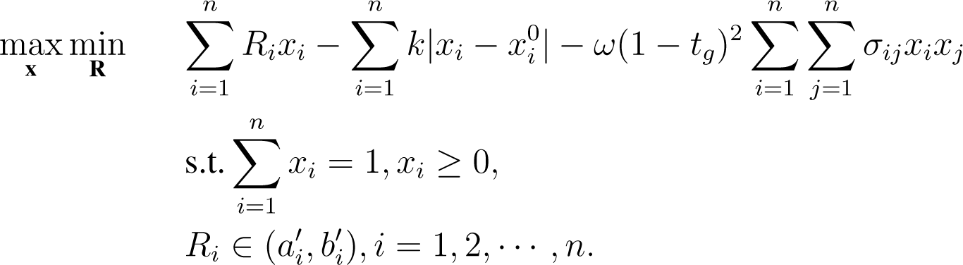
Based on the mean-variance framework, in our model we attempt to maximize the minimization over expected returns subject to the constraint that all of the asset expected returns lie within some specified intervals. Therefore, it can be formulated by the following min-max problem:

(1)

where the parameter ω ∈ [0, +∞) characterizes the investor’s risk aversion, ${a^{\prime }}_i=(1-t_g)a_i+(1-t_0)d_i$, ${b^{\prime }}_i=(1-t_g)b_i+(1-t_0)d_i$.

3. Optimal Strategy

In this section, we are devoted to finding the optimal solution to Problem (1). This problem is a standard min-max problem with linear constraints, which may be solved by using the maximum entropy method. It should be pointed out that the objective function including transaction costs and dividends is not differentiable, and the discrete maximum entropy algorithm in [6] can not be applied directly to the present problem. This paper proposes a continuous maximum entropy method to solve the problem. Next, we give a quick review of this method.

3.1. Maximum Entropy Method

We first consider the following min-max optimal problem:

$$\underset{x\in \omega }{min}\underset{y\in {\omega }^{\prime }}{max}f(x,y),$$

(2)

where x ∈ Ω ⊆ Rⁿ, y ∈ Ω′ = [0, N₁] × [0, N₂] × ⋯ [0, N_m] ⊂ R^m.

We define

$$z=\underset{y}{max}f(x,y),$$

(3)

$$g(x,y,z)=f(x,y)-z.$$

(4)

Obviously, Problem (2) is equivalent to the following optimization problem:

$$\begin{array}{l}minz\\ \mathrm{s}.\mathrm{t}.g(x,y,z)\le 0.\end{array}$$

(5)

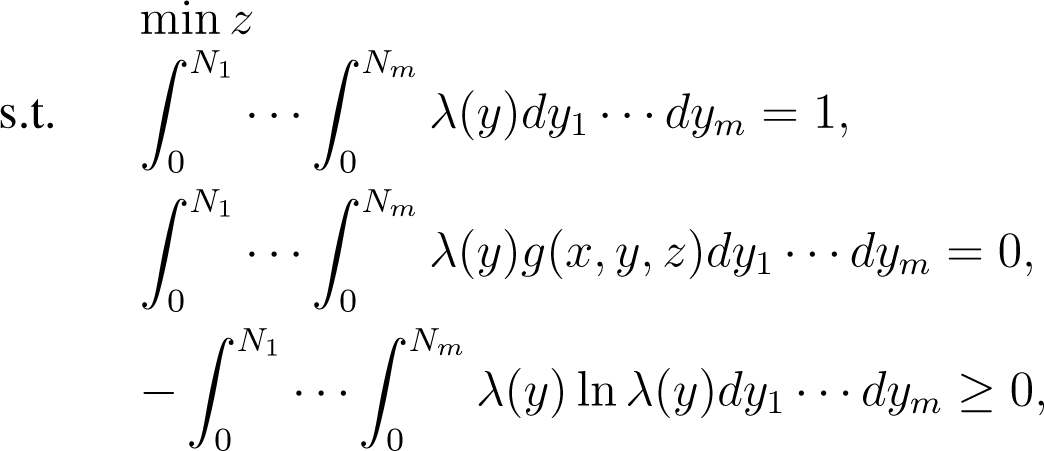
According to the results by Huang and Shen [18], and its references such as Shannon [19], Skilling and Gull [20], Everett [21], Brooks and Geoffrion [22], Gould [23] and Greenberg and Pierskalla [24], Problem (5) is equivalent to the following problem:

(6)

where λ(y) represents the probability density function of the y. The last constraint is the famous maximum entropy condition. In the following, we will provide the optimal probability density function λ^∗(y) of y according to the maximum entropy constraint.

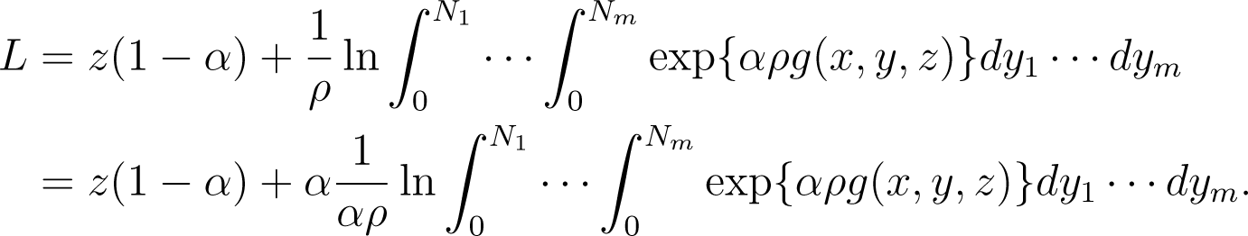
Then, the Lagrange function of Problem (6) can be expressed by

where α, μ, ρ > 0 are all the Lagrange multipliers.

Denote

$$T(x,\lambda (y))=\alpha \lambda (y)g(x,y,z)+\mu (\lambda (y)-\frac{1}{M})-\frac{1}{\rho }\lambda (y)\ln \lambda (y),$$

where $M={\displaystyle {\prod }_{i=1}^m{N}_i}$.

According to variational principle, it yields

$$\frac{\partial T(x,\lambda (y))}{\partial \lambda (y)}=0.$$

(7)

Since g(x, y, z) is unrelated to λ(y), it follows from (7) that

$$\alpha g(x,y,z)+\mu -\frac{1}{\rho }[\ln {\lambda }^{*}(y)+1]=0.$$

It is known from (6) that

$${\displaystyle {\int }_0^{N_1}\cdots {\displaystyle {\int }_0^{N_m}{\lambda }^{*}}(y)}d{y}_1\cdots d{y}_m=1.$$

(8)

Thus, it has the following system of equations:

$$\{\begin{array}{c}\alpha g(x,y,z)+\mu -\frac{1}{\rho }[\ln {\lambda }^{*}(y)+1]=0,\\ {\displaystyle {\int }_0^{N_1}\cdots }{\displaystyle {\int }_0^{N_m}{\lambda }^{*}}(y)d{y}_1\cdots d{y}_m=1.\end{array}$$

(9)

From the first equation of (9), we have

$${\lambda }^{*}(y)=\exp \{\alpha \rho g(x,y,z)\}\exp \{\rho \mu +1\}.$$

(10)

Substituting (10) into the second equation of (9), we get

$${\displaystyle {\int }_0^{N_1}\cdots }{\displaystyle {\int }_0^{N_m}\exp \{\alpha \rho g(x,y,z)\}\exp \{\rho \mu +1\}d{y}_1\cdots d{y}_m}=1.$$

Since exp{ρμ + 1} is a constant, it follows that

$$\exp \{\rho \mu +1\}=\frac{1}{{\displaystyle {\int }_0^{N_1}\cdots {\displaystyle {\int }_0^{N_m}\exp }\{\alpha \rho g(x,y,z)\}d{y}_1\cdots d{y}_m}}.$$

(11)

Hence, in view of (11) and (10), we obtain that

$${\lambda }^{*}(y)=\frac{\exp \{\alpha \rho g(x,y,z)\}}{{\displaystyle {\int }_0^{N_1}\cdots }{\displaystyle {\int }_0^{N_m}\exp \{\alpha \rho g(x,y,z)\}d{y}_1}\cdots d{y}_m}.$$

(12)

Substituting (12) into the original Lagrange function, we get

$$L=z+\frac{1}{\rho }\ln {\displaystyle {\int }_{\rho }^{N_1}\cdots }{\displaystyle {\int }_0^{N_m}\exp \{\alpha \rho g(x,y,z)\}d{y}_1\cdots d{y}_m}.$$

It follows from (3) and (4) that

Define

$$F_p(x):=\frac{1}{p}\ln {\displaystyle {\int }_0^{N_1}\cdots }{\displaystyle {\int }_0^{N_m}\exp \{pg(x,y,z)\}d{y}_1\cdots d{y}_m}.$$

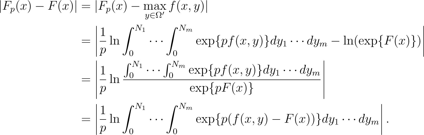
Obviously, F_p(x) is a multi-dimensional continuous maximum entropy function. We can derive that

$$L=z(1-\alpha )+\alpha F_p(x),$$

where p = αρ.

Define

$$F(x)=\underset{y\in {\omega }^{\prime }}{max}f(x,y).$$

Our main objective is to prove the convergence of L. If we can prove F_p(x) converges to F (x), then we can get the convergence of the function L. That means L converges to z(1 − α) + αF (x). We find that the value of α does not affect the convergence of L.

Without loss of generality, we set α = 1, then

$$L=F_p(x)=\frac{1}{p}\ln {\displaystyle {\int }_0^{N_1}\cdots }{\displaystyle {\int }_0^{N_m}\exp \{pg(x,y,z)\}d{y}_1\cdots d{y}_m.}$$

Theorem 4. For any m > 1 and p > 1, we have$\left|F_p(x)-F(x)\right|\le \left|\frac{\ln M}{p}\right|$. Moreover, if p → + ∞, then F_p(x) → F(x). Where$F_p\left(x\right)=\frac{1}{p}\ln {\displaystyle {\int }_0^{N_1}\cdots {\displaystyle {\int }_0^{N_m}\exp \left\{pf\left(x,y\right)\right\}d{y}_1\cdots d{y}_m,}}F\left(x\right)={max}_{y\in {\omega }^{\prime }}f\left(x,y\right),M={\displaystyle {\prod }_{i=1}^m{N}_i}$.

Proof. For any x ∈ Ω

Since

$$f\left(x,y\right)-F\left(x\right)=f\left(x,y\right)-\underset{y\in {\omega }^{\prime }}{max}f\left(x,y\right)\le 0,p>1,$$

then we obtain

$$p(f(x,y)-F(x))\le 0.$$

Moreover, we can deduce that

$$\exp \{p(f(x,y)-F(x))\}\le 1.$$

Hence, we arrive at

$$\left|F_p\left(x\right)-F\left(x\right)\right|\le \left|\frac{1}{p}\ln {\displaystyle {\int }_0^{N_1}\cdots {\displaystyle {\int }_0^{N_m}d{y}_1\cdots d{y}_m}}\right|\le \left|\frac{\ln M}{p}\right|.$$

Thus, F_p(x) → F (x), when p → +∞. □

3.2. Optimal Solution

Based on the discussion of subsection 3.1, now we aim to determine the solution of Problem (1). Since

$$\underset{x\in \omega }{max}\underset{y\in {\omega }^{\prime }}{min}f\left(x,y\right)=\left(-\underset{x\in \omega }{min}\right)\left(-\underset{y\in {\omega }^{\prime }}{max}\right)\left\{f\left(x,y\right)\right\}=\underset{x\in \omega }{min}\underset{y\in {\omega }^{\prime }}{max}f\left(x,y\right),$$

then Problem (1) can be reformulated as follows:

$$\begin{array}{l}\underset{\mathbf{x}}{min}\underset{\mathbf{R}}{max}{\displaystyle \sum _{i=1}^n\left({R^{\prime }}_i+{a^{\prime }}_i\right)x_i}-{\displaystyle \sum _{i=1}^{n}k\left|x_i-x_i^0\right|-\omega {\left(1-t_g\right)}^2}{\displaystyle \sum _{i=1}^n{\displaystyle \sum _{j=1}^n{\sigma }_{ij}{x}_i{x}_j}}\\ \mathrm{s}.\mathrm{t}.{\displaystyle \sum _{i=1}^n{x}_i=1,}{x}_i\ge 0,\\ {R^{\prime }}_i\in \left[0,{b^{\prime }}_i-{a^{\prime }}_i\right],i=1,2,\cdots ,n.\end{array}$$

(13)

where ${R^{\prime }}_i=R_i-{a^{\prime }}_i$.

It can be seen that min_x∈Ω F_p(x) is an approximation of Problem (13).

Let

$$h\left(x,R^{\prime }\right)=\exp \left\{p\left(-{\displaystyle \sum _{i=1}^n\left({R^{\prime }}_i+{a^{\prime }}_i\right)x_i}+{\displaystyle \sum _{i=1}^{n}k\left|x_i-x_i^0\right|+\omega {(1-t_g)}^2}{\displaystyle \sum _{i=1}^n{\displaystyle \sum _{j=1}^n{\sigma }_{ij}{x}_i{x}_j}}\right)\right\}.$$

According to Theorem 4, Problem (13) can be approximated by the following constrained optimization problem:

$$\begin{array}{l}\underset{x}{min}\left\{-\frac{1}{p}\ln {\displaystyle {\int }_0^{{b^{\prime }}_1-{a^{\prime }}_1}\cdots }{\displaystyle {\int }_0^{{b^{\prime }}_n-{a^{\prime }}_n}h\left(x,R^{\prime }\right)d{R^{\prime }}_1\cdots d{R^{\prime }}_n}\right\}\\ \mathrm{s}.\mathrm{t}.{\displaystyle \sum _{i=1}^n{x}_i=1,x_i\ge 0.}\end{array}$$

(14)

For the sake of convenience, denote

$$T_1={\displaystyle \sum _{i=1}^n{\displaystyle \sum _{j=1}^n\omega {\left(1-t_g\right)}^2{\sigma }_{ij}{x}_i{x}_j},}$$

(15)

$$T_2={\displaystyle \sum _{i=1}^{n}k\left|x_i-x_i^0\right|}.$$

(16)

Therefore, Problem (14) can be re-written as

$$\begin{array}{l}\underset{x}{min}\left\{-\frac{1}{p}\ln {\displaystyle {\int }_0^{{b^{\prime }}_1-{a^{\prime }}_1}\cdots }{\displaystyle {\int }_0^{{b^{\prime }}_n-{a^{\prime }}_n}\exp \left\{p\left({\displaystyle \sum _{i=1}^n\left({R^{\prime }}_i+{a^{\prime }}_i\right)x_i}\right)-T_1-T_2\right\}d{R^{\prime }}_1\cdots d{R^{\prime }}_n}\right\}\\ =\underset{x}{min}\left\{-\frac{1}{p}\ln {\displaystyle {\int }_0^{{b^{\prime }}_1-{a^{\prime }}_1}\cdots }{\displaystyle {\int }_0^{{b^{\prime }}_n-{a^{\prime }}_n}\exp \left\{p\left({\displaystyle \sum _{i=1}^n\left({R^{\prime }}_i+{a^{\prime }}_i\right)x_i}\right)\right\}d{R^{\prime }}_1\cdots d{R^{\prime }}_n+T_1+T_2}\right\}.\end{array}$$

(17)

Substituting both (15) and (16) into (17), Problem (14) can be reformulated as follows:

$$\begin{array}{l}\underset{x}{min}\left\{-\frac{1}{p}\left(\ln \frac{1}{x_1\cdots x_n{p}^n}+{\displaystyle \sum _{i=1}^n\ln \left(e^{p{b^{\prime }}_i{x}_i}-e^{p{a^{\prime }}_i{x}_i}\right)}\right)+{\displaystyle \sum _{i=1}^{n}k\left|x_i-x_i^0\right|}+{\displaystyle \sum _{i=1}^n{\displaystyle \sum _{j=1}^n\omega {(1-t_g)}^2{\sigma }_{ij}{x}_i{x}_j}}\right\}\\ \mathrm{s}.\mathrm{t}.{\displaystyle \sum _{i=1}^n{x}_i=1,}{x}_i\ge 0.\end{array}$$

(18)

Obviously, Problem (18) is a non-smooth optimization problem. So the derivative of the objective function does not exist at some point. Thus, a derivative-free method is needed to solve this problem. In this paper, we adopt the widely used simplex search method (Lagarias et al. [25]), which is available in Matlab by the subroutine ‘fmincon’.

4. Computational Results

In order to test the performance of robust mean-variance model, we consider a real portfolio which selects six stocks of historical data from Shanghai Stock Exchange. Original data of six stocks from each week’s closing prices from January in 2009 to May in 2014. As a result, the covariance matrix of six stocks is as follows:

$$\left(\begin{array}{cccccc}0.004335& 0.001100& 0.000703& 0.001547& 0.001095& 0.000804\\ 0.001100& 0.004665& 0.001177& 0.000987& 0.001318& 0.000617\\ 0.000703& 0.001177& 0.005983& 0.000816& 0.000599& 0.000939\\ 0.001547& 0.000987& 0.000816& 0.003932& 0.000865& 0.001323\\ 0.001095& 0.001318& 0.000599& 0.000865& 0.005597& 0.000324\\ 0.000804& 0.000617& 0.000939& 0.001323& 0.000324& 0.002040\end{array}\right)$$

The week’s expected returns and their estimated intervals are listed in

Table 1. The week’s expected returns of six stocks.

Code	000581	002041	600362	600252	600406	600021
Mean	0.00785	0.005028	0.005744	0.001903	0.001422	0.00222

and

Table 2. The estimated intervals of week’s expected returns.

Code	000581	002041	600362	600252	600406	600021
Range	(0.0061, 0.0109)	(0.0038, 0.0076)	(0.0040, 0.0088)	(0.0005, 0.0052)	(0.0004, 0.0040)	(0.0011, 0.0052)

.

4.1. Comparison with a Classical Mean-Variance Model

The classical mean-variance model under the same market situation of this paper can be formulated as follows:

$$\begin{array}{l}\underset{\mathrm{x}}{max}{\displaystyle \sum _{i=1}^n{R}_i{x}_i}-{\displaystyle \sum _{i=1}^{n}k\left|x_i-x_i^0\right|-\omega {\left(1-t_g\right)}^2}{\displaystyle \sum _{i=1}^n{\displaystyle \sum _{j=1}^n{\sigma }_{ij}{x}_i{x}_j}}\\ \mathrm{s}.\mathrm{t}.{\displaystyle \sum _{i=1}^n{x}_i=1,x_i\ge 0,i=1,2,\cdots ,n.}\end{array}$$

(19)

where the notations of mathematical symbols are the same as this paper.

Now, we provide the market performances for the classical mean-variance model and the robust one. Let’s assign the following parameters: p = 30000, t_g = 0.3, t_s = 0.00002, t_f = 0.00007. For simplification, we set $x_i^0=0$.

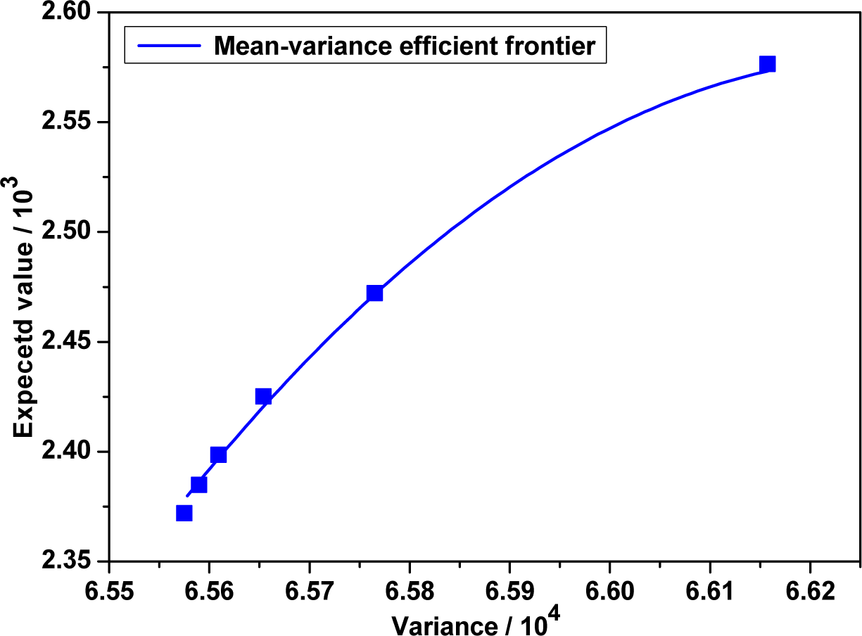
By using the subroutine “fmincon”in Matlab, we obtain the optimal strategies, efficient points and efficient frontier of classical mean-variance model in the following

Table 3. The optimal strategies and efficient points corresponding to risk aversion ω.

ω	x*	(V ar(x*), E(x*))
20	(0.1726, 0.1344, 0.1083, 0.0347, 0.1173, 0.4327)	(0.0006631, 0.002608)
35	(0.1507, 0.1297, 0.1011, 0.0426, 0.1274, 0.4485)	(0.0006581, 0.002487)
50	(0.1415, 0.1273, 0.0968, 0.0441, 0.1320, 0.4583)	(0.0006567, 0.002433)
65	(0.1363, 0.1257, 0.0941, 0.0443, 0.1341, 0.4655)	(0.0006561, 0.002401)
80	(0.1332, 0.1243, 0.0931, 0.0474, 0.1364, 0.4656)	(0.0006559, 0.002382)
100	(0.1308, 0.1238, 0.0926, 0.0488, 0.1374, 0.4666)	(0.0006557, 0.002370)

and Figure 1 respectively.

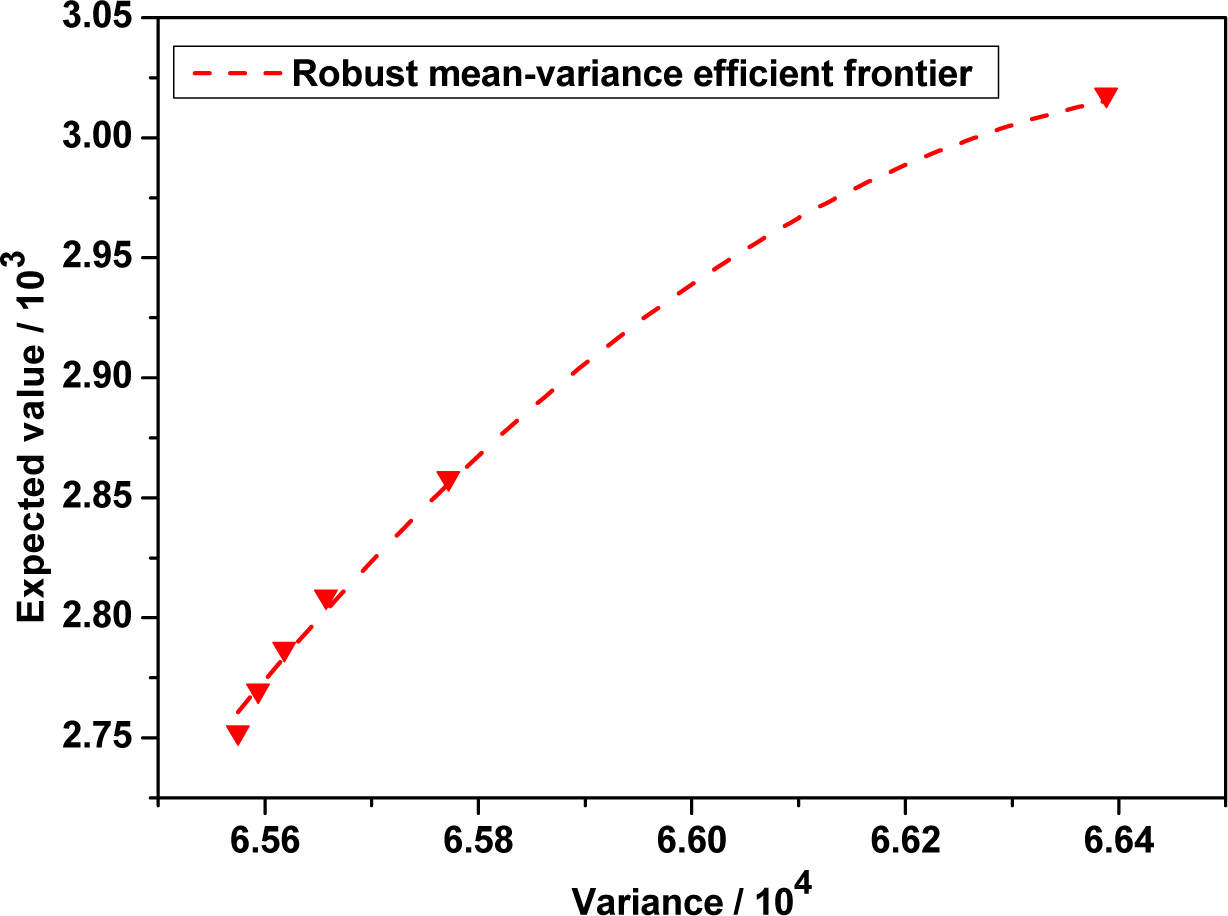
By using the maximum entropy method and subroutine ‘fmincon’ in Matlab, we obtain the optimal strategies, efficient points and efficient frontier of robust mean-variance model in the following

Table 4. The optimal strategies and efficient points corresponding to risk aversion ω.

ω	X*	(V ar(x*), E(x*))
20	(0.1762, 0.1335, 0.1047, 0.0184, 0.1191, 0.4481)	(0.0006635, 0.003011)
35	(0.1501, 0.1293, 0.0988, 0.0370, 0.1284, 0.4564)	(0.0006579, 0.002864)
50	(0.1423, 0.1262, 0.0958, 0.0409, 0.1316, 0.4632)	(0.0006567, 0.002816)
65	(0.1369, 0.1247, 0.0934, 0.0422, 0.1338, 0.4690)	(0.0006562, 0.002785)
80	(0.1330, 0.1238, 0.0915, 0.0443, 0.1350, 0.4724)	(0.0006559, 0.002762)
100	(0.1312, 0.1231, 0.0926, 0.0477, 0.1371, 0.4683)	(0.0006557, 0.002752)

and Figure 2 respectively.

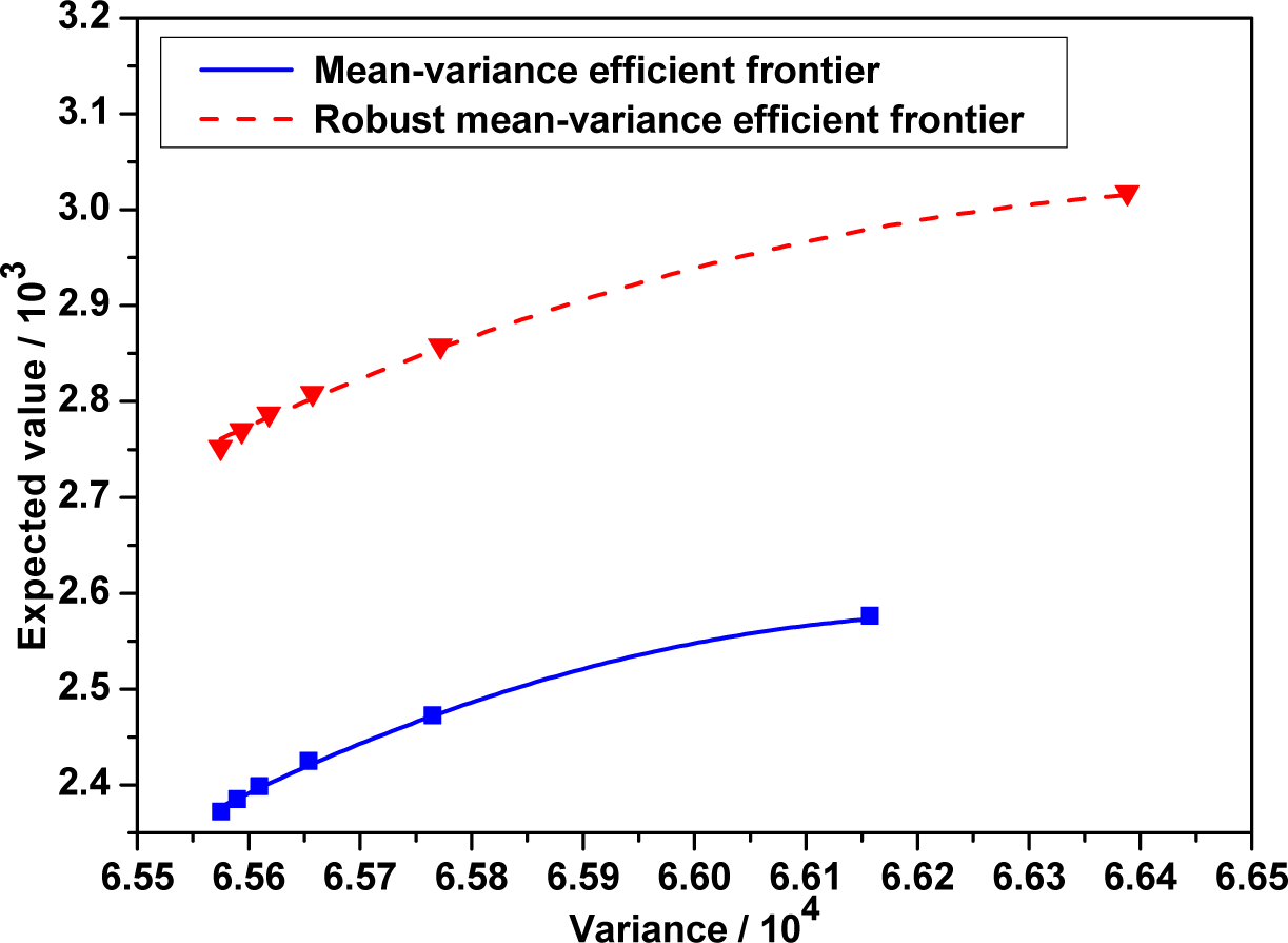
Next, we put the efficient frontiers of the robust mean-variance model and classical mean-variance model in the same coordinate plane.

Figure 3 shows the efficient frontiers to the robust model and classical mean-variance one. It indicates that the classical mean-variance efficient frontier lies far below the robust one. An immediate finding is that the investor selecting the mean-variance strategy must take more risk than one selecting the robust strategy under the same conditions of portfolio return. In other words, under the same conditions of portfolio risk, an investor selecting the mean-variance strategy has less return than one selecting the robust strategy. This means that the optimal portfolio in the mean-variance framework is not a good portfolio. More importantly, this robust portfolio strategy will help investors avoid excessive losses when unexpected events happen.

4.2. Comparison without Transaction Costs

The robust mean-variance model without transaction costs can be expressed as follows:

$$\begin{array}{l}\underset{\mathbf{x}}{max}\underset{\mathbf{r}}{min}{\displaystyle \sum _{i=1}^n{r}_i{x}_i-\omega {\displaystyle \sum _{i=1}^n{\displaystyle \sum _{j=1}^n{\sigma }_{ij}{x}_i{x}_j}}}\\ \mathrm{s}.\mathrm{t}.{\displaystyle \sum _{i=1}^n{x}_i=1,x_i\ge }0,\\ ri\in \left(a_i,b_i\right),i=1,2,\cdots ,n.\end{array}$$

(20)

where the notations of mathematical symbols are the same as this paper.

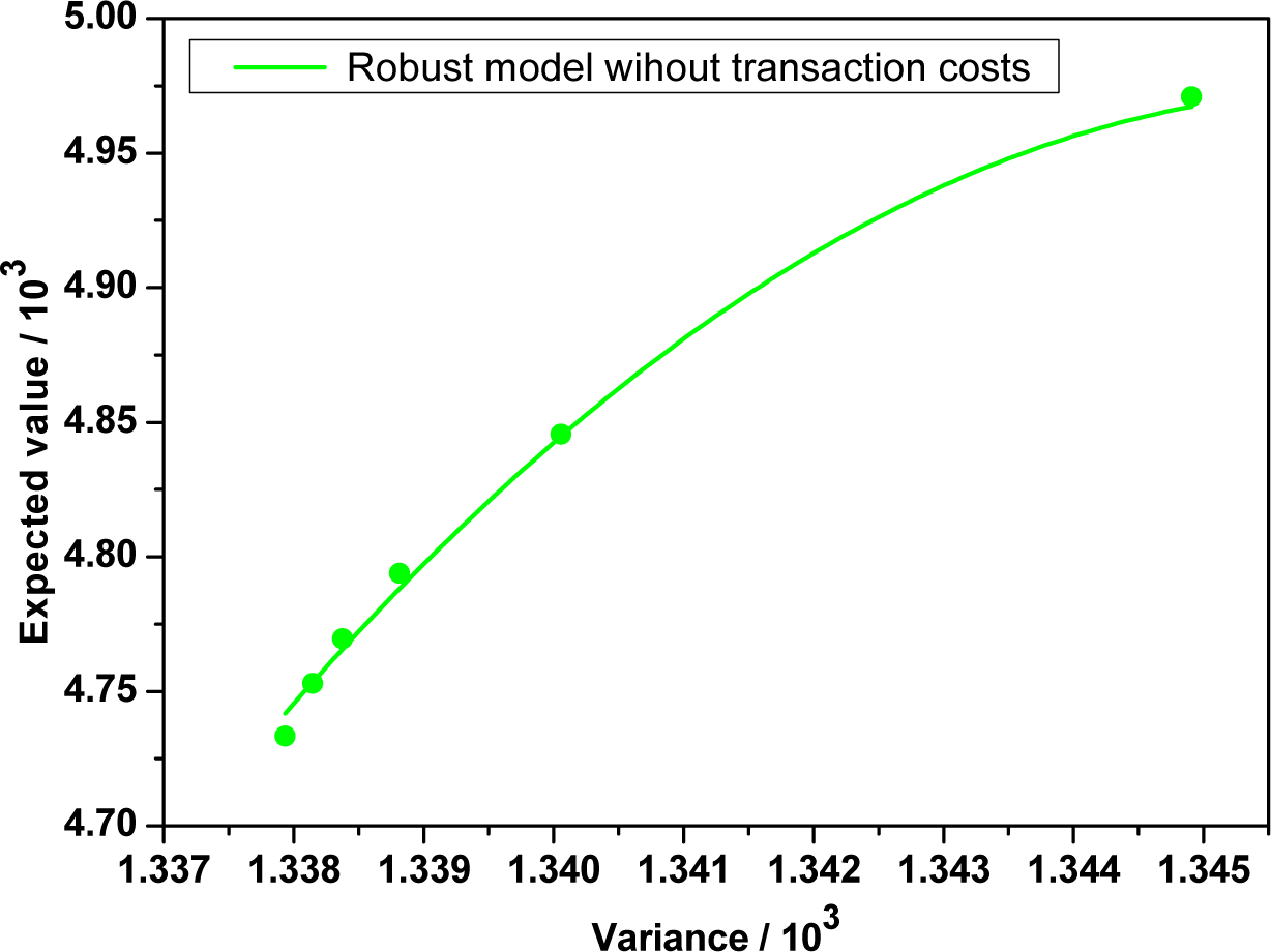
By using the maximum entropy method and subroutine “fmincon” in Matlab, we obtain the optimal strategies, efficient points and efficient frontier of robust mean-variance model without transaction costs in the following

Table 5. The optimal strategies and efficient points corresponding to risk aversion ω.

ω	X*	(V ar(x*), E(x*))
20	(0.1580, 0.1299, 0.1006, 0.0308, 0.1255, 0.4551)	(0.001345, 0.004979)
35	(0.1410, 0.1257, 0.0943, 0.0397, 0.1315, 0.4678)	(0.001340, 0.004839)
50	(0.1355, 0.1238, 0.0940, 0.0459, 0.1352, 0.4656)	(0.001339, 0.004794)
65	(0.1313, 0.1243, 0.0924, 0.0485, 0.1358, 0.4677)	(0.001338, 0.004764)
80	(0.1301, 0.1235, 0.0924, 0.0486, 0.1372, 0.4682)	(0.001338, 0.004753)
100	(0.1283, 0.1231, 0.0920, 0.0494, 0.1381, 0.4691)	(0.001337, 0.004740)

and Figure 4 respectively.

Comparing Table 4 with Table 5, we find that transaction costs play as a penalty factor for portfolio revision. Furthermore, it tells us that the impact of transaction costs can not be ignored in the real world when portfolio managers choose investment strategy.

5. Conclusions

This paper provides a maximum entropy method to investigate the robust optimal portfolio selection problem for the market with transaction costs and dividends. For avoiding the sensitivity of optimal portfolio to input data such as expected return and variance, we restrict the asset expected return to lie within a specified interval. By maximizing the minimization over expected returns, we naturally establish our robust portfolio model. We find that this problem can be solved by using a continuous maximum entropy method. The numerical experiments indicate that the robust portfolio model is achieved at relatively good performance than the classical mean-variance ones. In addition, we consider the market with transaction costs and dividends, which is an important concern for investors. The research on multi-period robust models and other risk measures instead of variance under this market circumstance is left for future work.

References

- Markowitz, H. Portfolio selection. J. Financ 1952, 7, 77–91. [Google Scholar]
- Markowitz, H. Portfolio Selection: Efficient Diversification of Investments; Wiley: New York, NY, USA, 1959. [Google Scholar]
- Konno, H.; Morita, Y.; Yamamoto, H. A maximal predictability portfolio absolute deviation reformulation. Comput. Manag. Sci 2001, 7, 47–60. [Google Scholar]
- Young, M.R. A minimax portfolio selection rule with linear programming solution. Manag. Sci 1998, 44, 673–683. [Google Scholar]
- Steinbach, M.C. Markowitz revisited: Mean-variance models in financial portfolio analysis. SIAM Rev 2001, 43, 31–85. [Google Scholar]
- Wu, Z.; Song, X.; Xu, Y.; Liu, K. A note on a minimax rule for portfolio selection and equilibrium price system. Appl. Math. Comput 2007, 208, 49–57. [Google Scholar]
- Best, M.J.; Grauer, R.R. On the sensitivity of mean-variance-efficient portfolios to changes in asset means: Some analytical and computational results. Rev. Financ. Stud 1991, 4, 315–342. [Google Scholar]
- Broadie, M. Computing efficient frontiers using estimated parameters. Ann. Oper. Res 1993, 45, 341–365. [Google Scholar]
- Black, F.; Litterman, R. Asset Allocation: Combining Investor Views with Market Equilibrium; Technical Report; Goldman Sachs: New York, NY, USA, 1990. [Google Scholar]
- Soyster, A. Convex programming with set-inclusive constraints and applications to inexact linear programming. Oper. Res 1973, 21, 1151–1154. [Google Scholar]
- Goldfarb, D.; Lyengar, G. Robust portfolio selection problems. Math. Oper. Res 2003, 29, 1–38. [Google Scholar]
- Ceria, S.; Stubbs, R.A. Incorporating estimation errors into portfolio selection: Robust portfolio construction. J. Asset Manag 2006, 7, 109–127. [Google Scholar]
- Ben-Tal, A.; Nemirovski, A. Robust solutions of linear programming problems contaminated with uncertain data. Math. Program 2000, 88, 411–424. [Google Scholar]
- Mansini, R.; Speranza, G. An exact approach for portfolio selection with transaction costs and rounds. IIE Trans 2005, 37, 919–929. [Google Scholar]
- Best, M.J.; Hlouskova, J. Portfolio selection and transactions costs. Comput. Optim. Appl 2003, 24, 95–116. [Google Scholar]
- Lobo, M.S.; Fazel, M.; Boyd, S. Portfolio optimization with linear and fixed transaction costs. Ann. Oper. Res 2007, 152, 341–365. [Google Scholar]
- Bertsimas, D.; Lo, A.W. Optimal control of execution costs. J. Financ. Mark 1998, 1, 1–50. [Google Scholar]
- Huang, Z.; Shen, Z. A maximum entropy method to a class of minmax problem. Chin. Sci. Bull 1996, 41, 1550–1554. (in Chinese). [Google Scholar]
- Shannon, C. A mathematical theory of Communication. Bell Syst. Tech. J 1948, 27, 379–428. [Google Scholar]
- Skilling, J.; Gull, S.F. Algorithm and its Application. In Maximum-Entropy and Bayesian Method in Inverse Problems; Smith, C.R., Grandy, W.T., Eds.; Reidel: Dordrecht, The Netherlands, 1985; pp. 83–132. [Google Scholar]
- Everett, H. Generalized Lagrange multiplier method for solving problems of optimum of resouces. Oper. Res 1963, 11, 399–417. [Google Scholar]
- Brooks, R.; Geoffrion, A. Finding Everett’s Lagrange multipliers by linear programming. Oper. Res 1966, 14, 1149–1153. [Google Scholar]
- Gould, F.J. Extensions of Lagrange multipliers in nonlinear programming. SIAM J. Appl. Math 1969, 17, 1280–1297. [Google Scholar]
- Greenberg, H.J.; Pierskalla, W.P. Surrogate mathematical programming. Oper. Res 1970, 18, 924–939. [Google Scholar]
- Lagarias, J.C.; Reeds, J.A.; Wright, M.H.; Wright, P.E. Convergence properties of the Nelder–Mead simplex method in low dimensions. SIAM J. Optim 1998, 9, 112–147. [Google Scholar]