Extending the Extreme Physical Information to Universal Cognitive Models via a Confident Information First Principle

Abstract

The principle of extreme physical information (EPI) can be used to derive many known laws and distributions in theoretical physics by extremizing the physical information loss K, i.e., the difference between the observed Fisher information I and the intrinsic information bound J of the physical phenomenon being measured. However, for complex cognitive systems of high dimensionality (e.g., human language processing and image recognition), the information bound J could be excessively larger than I (J≫I), due to insufficient observation, which would lead to serious over-fitting problems in the derivation of cognitive models. Moreover, there is a lack of an established exact invariance principle that gives rise to the bound information in universal cognitive systems. This limits the direct application of EPI. To narrow down the gap between I and J, in this paper, we propose a confident-information-first (CIF) principle to lower the information bound J by preserving confident parameters and ruling out unreliable or noisy parameters in the probability density function being measured. The confidence of each parameter can be assessed by its contribution to the expected Fisher information distance between the physical phenomenon and its observations. In addition, given a specific parametric representation, this contribution can often be directly assessed by the Fisher information, which establishes a connection with the inverse variance of any unbiased estimate for the parameter via the Cramér–Rao bound. We then consider the dimensionality reduction in the parameter spaces of binary multivariate distributions. We show that the single-layer Boltzmann machine without hidden units (SBM) can be derived using the CIF principle. An illustrative experiment is conducted to show how the CIF principle improves the density estimation performance.

1. Introduction

Information has been found to play an increasingly important role in physics. As stated in Wheeler [1]: “All things physical are information-theoretic in origin and this is a participatory universe...Observer participancy gives rise to information; and information gives rise to physics”. Following this viewpoint, Frieden [2] unifies the derivation of physical laws in major fields of physics, from the Dirac equation to the Maxwell-Boltzmann velocity dispersion law, using the extreme physical information principle (EPI). More specifically, a variety of equations and distributions can be derived by extremizing the physical information loss K, i.e., the difference between the observed Fisher information I and the intrinsic information bound J of the physical phenomenon being measured.

The first quantity, I, measures the amount of information as a finite scalar implied by the data with some suitable measure [2]. It is formally defined as the trace of the Fisher information matrix [3]. In addition to I, the second quantity, the information bound J, is an invariant that characterizes the information that is intrinsic to the physical phenomenon [2]. During the measurement procedure, there may be some loss of information, which entails I = κJ, where κ ≤ 1 is called the efficiency coefficient of the EPI process in transferring the Fisher information from the phenomenon (specified by J) to the output (specified by I). For closed physical systems, in particular, any solution for I attains some fraction of J between 1/2 (for classical physics) and one (for quantum physics) [4].

However, it is usually not the case in cognitive science. For complex cognitive systems (e.g., human language processing and image recognition), the target probability density function (pdf) being measured is often of high dimensionality (e.g., thousands of words in a human language vocabulary and millions of pixels in an observed image). Thus, it is infeasible for us to obtain a sufficient collection of observations, leading to excessive information loss between the observer and nature. Moreover, there is a lack of an established exact invariance principle that gives rise to the bound information in universal cognitive systems. This limits the direct application of EPI in cognitive systems.

In terms of statistics and machine learning, the excessive information loss between the observer and nature will lead to serious over-fitting problems, since the insufficient observations may not provide necessary information to reasonably identify the model and support the estimation of the target pdf in complex cognitive systems. Actually, a similar problem is also recognized in statistics and machine learning, known as the model selection problem [5]. In general, we would require a complex model with a high-dimensional parameter space to sufficiently depict the original high-dimensional observations. However, over-fitting usually occurs when the model is excessively complex with respect to the given observations. To avoid over-fitting, we would need to adjust the complexity of the models to the available amount of observations and, equivalently, to adjust the information bound J corresponding to the observed information I.

In order to derive feasible computational models for cognitive phenomenon, we propose a confident-information-first (CIF) principle in addition to EPI to narrow down the gap between I and J (thus, a reasonable efficiency coefficient κ is implied), as illustrated in Figure 1. However, we do not intend to actually derive the distribution laws by solving the differential equations of the extremization of the new information loss K′. Instead, we assume that the target distribution belongs to some general multivariate binary distribution family and focus on the problem of seeking a proper information bound with respect to the constraint of the parametric number and the given observations.

The key to the CIF approach is how to systematically reduce the physical information bound for high-dimensional complex systems. As stated in Frieden [2], the information bound J is a functional form that depends upon the physical parameters of the system. The information is contained in the variations of the observations (often imperfect, due to insufficient sampling, noise and intrinsic limitations of the “observer”), and can be further quantified using the Fisher information of system parameters (or coordinates) [3] from the estimation theory. Therefore, the physical information bound J of a complex system can be reduced by transforming it to a simpler system using some parametric reduction approach. Assuming there exists an ideal parametric model S that is general enough to represent all system phenomena (which gives the ultimate information bound in Figure 1), our goal is to adopt a parametric reduction procedure to derive a lower-dimensional sub-model M (which gives the reduced information bound in Figure 1) for a given dataset (usually insufficient or perturbed by noises) by reducing the number of free parameters in S.

Formally speaking, let q(ξ) be the ideal distribution with parameters ξ that describes the physical system and q(ξ + Δξ) be the observations of the system with some small fluctuation Δξ in parameters. In [6], the averaged information distance I(Δξ) between the distribution and its observations, the so-called shift information, is used as a disorder measure of the fluctuated observations to reinterpret the EPI principle. More specifically, in the framework of information geometry, this information distance could also be assessed using the Fisher information distance induced by the Fisher–Rao metric, which can be decomposed into the variation in the direction of each system parameter [7]. In principle, it is possible to divide system parameters into two categories, i.e., the parameters with notable variations and the parameters with negligible variations, according to their contributions to the whole information distance. Additionally, the parameters with notable contributions are considered to be confident, since they are important for reliably distinguishing the ideal distribution from its observation distributions. On the other hand, the parameters with negligible contributions can be considered to be unreliable or noisy. Then, the CIF principle can be stated as the parameter selection criterion that maximally preserves the Fisher information distance in an expected sense with respect to the constraint of the parametric number and the given observations (if available), when projecting distributions from the parameter space of S into that of the reduced sub-model M. We call it the distance-based CIF. As a result, we could manipulate the information bound of the underlying system by preserving the information of confident parameters and ruling out noisy parameters.

In this paper, the CIF principle is analyzed in the multivariate binary distribution family in the mixed-coordinate system [8]. It turns out that, in this problematic configuration, the confidence of a parameter can be directly evaluated by its Fisher information, which also establishes a connection with the inverse variance of any unbiased estimate for the parameter via the Cramér–Rao bound [3]. Hence, the CIF principle can also be interpreted as the parameter selection procedure that keeps the parameters with reliable estimates and rules out unreliable or noisy parameters. This CIF is called the information-based CIF. Note that the definition of confidence in distance-based CIF depends on both Fisher information and the scale of fluctuation, and the confidence in the information-based CIF (i.e., Fisher information) can be seen as a special case of confidence measure with respect to certain coordinate systems. This simplification allows us to further apply the CIF principle to improve existing learning algorithms for the Boltzmann machine.

The paper is organized as follows. In Section 2, we introduce the parametric formulation for the general multivariate binary distributions in terms of information geometry (IG) framework [7]. Then, Section 3 describes the implementation details of the CIF principle. We also give a geometric interpretation of CIF by showing that it can maximally preserve the expected information distance (in Section 3.2.1), as well as the analysis on the scale of the information distance in each individual system parameter (in Section 3.2.2). In Section 4, we demonstrate that a widely used cognitive model, i.e., the Boltzmann machine, can be derived using the CIF principle. Additionally, an illustrative experiment is conducted to show how the CIF principle can be utilized to improve the density estimation performance of the Boltzmann machine in Section 5.

2. The Multivariate Binary Distributions

Similar to EPI, the derivation of CIF depends on the analysis of the physical information bound, where the choice of system parameters, also called “Fisher coordinates” in Frieden [2], is crucial. Based on information geometry (IG) [7], we introduce some choices of parameterizations for binary multivariate distributions (denoted as statistical manifold S) with a given number of variables n, i.e., the open simplex of all probability distributions over binary vector x ∈{0, 1}ⁿ.

2.1. Notations for Manifold S

In IG, a family of probability distributions is considered as a differentiable manifold with certain parametric coordinate systems. In the case of binary multivariate distributions, four basic coordinate systems are often used: p-coordinates, η-coordinates, θ-coordinates and mixed-coordinates [7,9]. Mixed-coordinates is of vital importance for our analysis.

For the p-coordinates [p] with n binary variables, the probability distribution over 2ⁿ states of x can be completely specified by any 2ⁿ − 1 positive numbers indicating the probability of the corresponding exclusive states on n binary variables. For example, the p-coordinates of n =2 variables could be [p] = (p₀₁,p₁₀,p₁₁). Note that IG requires all probability terms to be positive [7].

For simplicity, we use the capital letters I, J, . . . to index the coordinate parameters of probabilistic distribution. To distinguish the notation of Fisher information (conventionally used in literature, e.g., data information I and information bound J in Section 1) from the coordinate indexes, we make explicit explanations when necessary from now on. An index I can be regarded as a subset of {1, 2,...,n}. Additionally, p_I stands for the probability that all variables indicated by I equal to one and the complemented variables are zero. For example, if I = {1, 2, 4} and n = 4, then p_I = p₁₁₀₁ = Prob (x₁ = 1, x₂ = 1, x₃ = 0, x₄ = 1). Note that the null set can also be a legal index of the p-coordinates, which indicates the probability that all variables are zero, denoted as p_0...0.

Another coordinate system often used in IG is η-coordinates, which is defined by:

$${\eta }_I=E[X_I]=\mathit{Prob}\left\{\prod _{i\in I}{x}_i=1\right\}$$

(1)

where the value of X_I is given by Π_i∈I x_i and the expectation is taken with respect to the probability distribution over x. Grouping the coordinates by their orders, the η-coordinate system is denoted as $[\eta ]=\left({\eta }_i^1,{\eta }_{ij}^2,\dots ,{\eta }_{1,2\dots n}^n\right)$, where the superscript indicates the order number of the corresponding parameter. For example, ${\eta }_{ij}^2$ denotes the set of all η parameters with the order number two.

The θ-coordinates (natural coordinates) are defined by:

$$\text{log}p(x)=\sum _{I\subseteq \{1,2,\dots ,n\},I\ne \mathit{NullSet}}{\theta }^I{X}_I-\psi (\theta )$$

(2)

where ψ(θ) = log(Σ_x exp{Σ_I θ^IX_I(x)}) is the cumulant generating function and its value equals to −log Prob{x_i =0, ∀i ∈{1, 2, ..., n}}. The θ-coordinate is denoted as $\left[\theta \right]=\left({\theta }_1^i,{\theta }_2^{ij},\dots ,{\theta }_n^{1,\dots ,n}\right)$, where the subscript indicates the order number of the corresponding parameter. Note that the order indices locate at different positions in [η] and [θ] following the convention in Amari et al. [8].

The relation between coordinate systems [η] and [θ] is bijective. More formally, they are connected by the Legendre transformation:

$${\theta }^I=\frac{\partial \varphi (\eta )}{\partial {\eta }_I},{\eta }_I=\frac{\partial \psi (\theta )}{\partial {\theta }^I}$$

(3)

where ψ(θ) is given in Equation (2) and ϕ(η) = Σ_x p(x; η) log p(x; η) is the negative of entropy. It can be shown that ψ(θ) and ϕ(η) meet the following identity [7]:

$$\psi (\theta )+\varphi (\eta )-\sum {\theta }^I{\eta }_I=0$$

(4)

Next, we introduce mixed-coordinates, which is important for our derivation of CIF. In general, the manifold S of probability distributions could be represented by the l-mixed-coordinates [8]:

$${[\zeta ]}_l=\left({\eta }_i^1,{\eta }_{ij}^2,\dots ,{\eta }_{i,j,\dots ,k}^l,{\theta }_{l+1}^{i,j,\dots ,k},\dots ,{\theta }_n^{1,\dots ,n}\right)$$

(5)

where the first part consists of η-coordinates with order less or equal to l (denoted by [η^l−]) and the second part consists of θ-coordinates with order greater than l (denoted by [θ_l+]), l ∈{1, ..., n − 1}.

2.2. Fisher Information Matrix for Parametric Coordinates

For a general coordinate system [ξ], the i-th row and j-th column element of the Fisher information matrix for [ξ] (denoted by G_ξ) is defined as the covariance of the scores of [ξ_i] and [ξ_j] [3], i.e.,

$$g_{ij}=E\left[\frac{\partial \text{log}p(x;\xi )}{\partial {\xi }_i}\cdot \frac{\partial \text{log}p(x;\xi )}{\partial {\xi }_j}\right]$$

under the regularity condition for the pdf that the partial derivatives exist. The Fisher information measures the amount of information in the data that a statistic carries about the unknown parameters [10]. The Fisher information matrix is of vital importance to our analysis, because the inverse of Fisher information matrix gives an asymptotically tight lower bound to the covariance matrix of any unbiased estimate for the considered parameters [3]. Another important concept related to our analysis is the orthogonality defined by Fisher information. Two coordinate parameters ξ_i and ξ_j are called orthogonal if and only if their Fisher information vanishes, i.e., g_ij = 0, meaning that their influences on the log likelihood function are uncorrelated.

The Fisher information for [θ] can be rewritten as $g_{IJ}=\frac{{\partial }^2\psi \left(\theta \right)}{\partial {\theta }^I\partial {\theta }^J}$, and for [η], it is $g^{IJ}=\frac{{\partial }^2\varphi \left(\theta \right)}{\partial {\eta }_I\partial {\eta }_J}$[7]. Let G_θ = (g_IJ) and G_n = (g^IJ) be the Fisher information matrices for [θ] and [η], respectively. It can be shown that G_θ and G_η are mutually inverse matrices, i.e., ${\Sigma }_J{g}^{IJ}{g}_{jk}={\delta }_K^I$, where ${\delta }_K^I=1$ if I = K and zero otherwise [7]. In order to generally compute G_θ and G_η, we develop the following Propositions 1 and 2. Note that Proposition 1 is a generalization of Theorem 2 in Amari et al. [8].

Proposition 1. The Fisher information between two parameters θ^I and θ^J in [θ], is given by:

$$g_{IJ}(\theta )={\eta }_{I\cup J}-{\eta }_I{\eta }_J$$

(6)

Proof. in Appendix A.

Proposition 2. The Fisher information between two parameters η_I and η_J in [η], is given by:

$$g^{IJ}(\eta )=\sum _{K\subseteq I\cap J}{\left(-1\right)}^{\left|I-K\right|+\left|J-K\right|}\cdot \frac{1}{pK}$$

(7)

where |·| denotes the cardinality operator.

Proof. in Appendix B.

Based on the Fisher information matrices G_η and G_θ, we can calculate the Fisher information matrix G_ζ for the l-mixed-coordinate system [ζ]_l, as follows:

Proposition 3. The Fisher information matrix G_ζ of the l-mixed-coordinates [ζ]_l is given by:

$$G_{\varsigma }=\left(\begin{array}{ll}A\hfill & 0\hfill \\ 0\hfill & B\hfill \end{array}\right)$$

(8)

where$A={\left({\left(G_{\eta }^{-1}\right)}_{I_{\eta }}\right)}^{-1}$, $B={\left({\left(G_{\theta }^{-1}\right)}_{J_{\theta }}\right)}^{-1}$, G_η and G_θ are the Fisher information matrices of [η] and [θ], respectively, I_η is the index set of the parameters shared by [η] and [ζ]_l, i.e., $\left\{{\eta }_i^1,\dots ,{\eta }_{i,j,\dots ,\kappa }^l\right\}$, and J_θ is the index set of the parameters shared by [θ] and [ζ]_l, i.e., $\left\{{\theta }_{l+1}^{i,j,\dots ,\kappa },\dots ,{\theta }_n^{l,\dots ,n}\right\}$.

Proof. in Appendix C.

3. The General CIF Principle

In this section, we propose the CIF principle to reduce the physical information bound for high-dimensionality systems. Given a target distribution q(x) ∈ S, we consider the problem of realizing it by a lower-dimensionality submanifold. This is defined as the problem of parametric reduction for multivariate binary distributions. The family of multivariate binary distributions has been proven to be useful when we deal with discrete data in a variety of applications in statistical machine learning and artificial intelligence, such as the Boltzmann machine in neural networks [11,12] and the Rasch model in human sciences [13,14].

Intuitively, if we can construct a coordinate system so that the confidences of its parameters entail a natural hierarchy, in which high confident parameters are significantly distinguished from and orthogonal to lowly confident ones, then we can conveniently implement CIF by keeping the high confident parameters unchanged and setting the lowly confident parameters to neutral values. Therefore, the choice of coordinates (or parametric representations) in CIF is crucial to its usage. This strategy is infeasible in terms of p-coordinates, η-coordinates or θ-coordinates, since the orthogonality condition cannot hold in these coordinate systems. In this section, we will show that the l-mixed-coordinates [ζ]_l meets the requirement of CIF.

In principle, the confidence of parameters should be assessed according to their contributions to the expected information distance between the ideal distribution and its fluctuated observations. This is called the distance-based CIF (see Section 1). For some coordinated systems, e.g., the mixed-coordinate system [ζ]_l, the confidence of a parameter can also be directly evaluated by its Fisher information. This is called the information-based CIF (see Section 1). The information-based CIF (i.e., Fisher information) can be seen as an approximation to distance-based CIF, since it neglects the influence of parameter scaling to the expected information distance. However, considering the standard mixed-coordinates [ζ]_l for the manifold of multivariate binary distributions, it turns out that both distance-based CIF and information-based CIF entail the same submanifold M (refer to Section 3.2 for detailed reasons).

For the purpose of legibility, we will start with the information-based CIF, where the parameter’s confidence is simply measured using its Fisher information. After that, we show that the information-based CIF leads to an optimal submanifold M, which is also optimal in terms of the more rigorous distance-based CIF.

3.1. The Information-Based CIF Principle

In this section, we will show that the l-mixed-coordinates [ζ]_l meet the requirement of the information-based CIF. According to Proposition 3 and the following Proposition 4, the confidences of coordinate parameters (measured by Fisher information) in [ζ]_l entail a natural hierarchy: the first part of high confident parameters [η^l−] are separated from the second part of low confident parameters [θ_l+]. Additionally, those low confident parameters [θ_l+] have the neutral value of zero.

Proposition 4. The diagonal elements of A are lower bounded by one, and those of B are upper bounded by one.

Proof. in Appendix D.

Moreover, the parameters in [η^l−] are orthogonal to the ones in [θ_l+], indicating that we could estimate these two parts independently [9]. Hence, we can implement the information-based CIF for parametric reduction in [ζ]_l by replacing low confident parameters with neutral value zero and reconstructing the resulting distribution. It turns out that the submanifold of S tailored by information-based CIF becomes ${\left[\zeta \right]}_{l_t}=\left({\eta }_i^1,\dots ,{\eta }_{ij\dots \kappa }^l,0,\dots ,0\right)$. We call [ζ]_lt the l-tailored-mixed-coordinates.

To grasp an intuitive picture for the CIF strategy and its significance w.r.t mixed-coordinates, let us consider an example with [p] = (p₀₀₁ = 0.15,p₀₁₀ = 0.1,p₀₁₁ = 0.05,p₁₀₀ = 0.2,p₁₀₁ = 0.1,p₁₁₀ =0.05,p₁₁₁ =0.3). Then, the confidences for coordinates in [η], [θ] and [ζ]₂ are given by the diagonal elements of the corresponding Fisher information matrices. Applying the two-tailored CIF in mixed-coordinates, the loss ratio of Fisher information is 0.001%, and the ratio of the Fisher information of the tailored parameter ( ${\theta }_3^{123}$) to the remaining η parameter with the smallest Fisher information is 0.06%. On the other hand, the above two ratios become 7.58% and 94.45% (in η-coordinates) or 12.94% and 92.31% (in θ-coordinates), respectively. We can see that [ζ]₂ gives us a much better way to tell apart confident parameters from noisy ones.

3.2. The Distance-Based CIF: A Geometric Point-of-View

In the previous section, the information-based CIF entails a submanifold of S determined by the l-tailored-mixed-coordinates [ζ]_lt. A more rigorous definition for the confidence of coordinates is the distance-based confidence used in the distance-based CIF, which relies on both of the coordinate’s Fisher information and its fluctuation scaling. In this section, we will show that the the submanifold M determined by [ζ]_lt is also an optimal submanifold M in terms of the distance-based CIF. Note that, for other coordinate systems (e.g., arbitrarily rescaling coordinates), the information-based CIF may not entail the same submanifold as the distance-based CIF.

Let q(x), with coordinate ζ_q, denote the exact solution to the physical phenomenon being measured. Additionally, the act of observation would cause small random perturbations to q(x), leading to some observation q′(x) with coordinate ζ_q+ Δζ_q. When two distributions q(x) and q′ (x) are close, the divergence between q(x) and q′ (x) on manifold S could be assessed by the Fisher information distance: D(q, q′) = (Δζ_q · G_ζ · Δζ_q)^1/2, where G_ζ is the Fisher information matrix and the perturbation Δζ_q′is small. The Fisher information distance between two close distributions q(x) and q′ (x) on manifold S is the Riemannian distance under the Fisher–Rao metric, which is shown to be the square root of the twice of the Kullback–Leibler divergence from q(x) to q′ (x) [8]. Note that we adopt the Fisher information distance as the distance measure between two close distributions, since it is shown to be the unique metric meeting a set of natural axioms for the distribution metrics [7,15,16], e.g., the invariant property with respect to reparametrizations and the monotonicity with respect to the random maps on variables.

Let M be a smooth k-dimensionality submanifold in S (k < 2ⁿ − 1). Given the point q(x) ∈ S, the projection [8] of q(x) on M is the point p(x) that belongs to M and is closest to q(x) with respect to the Kullback–Leibler divergence (K-L divergence) [17] from the distribution q(x) to p(x). 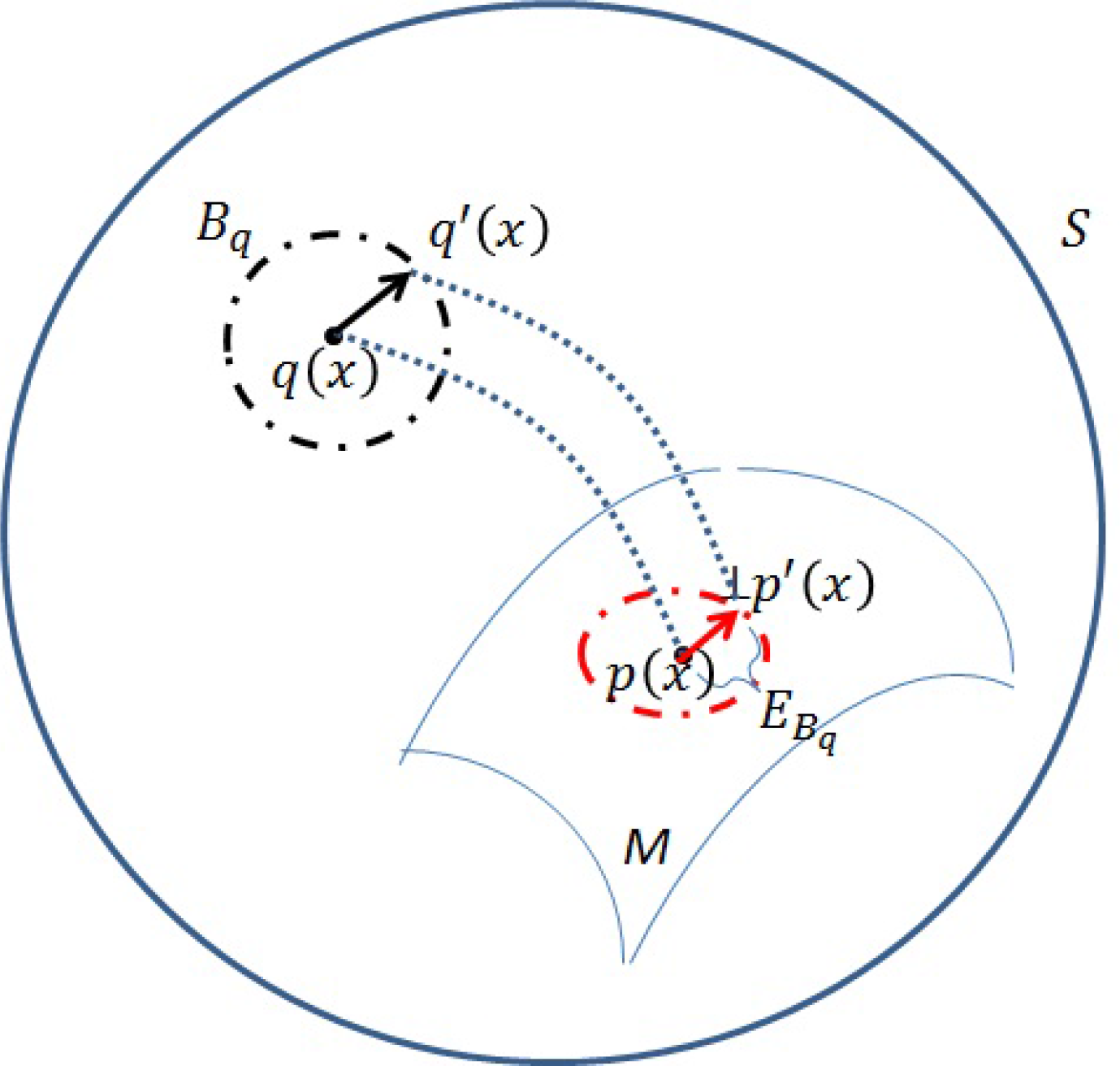On the submanifold M, the projections of q(x) and q′ (x) are p(x) and p′(x), with coordinates ζ_p and ζ_p + Δζ_p, respectively, shown in Figure 2.

Let the preserved Fisher information distance be D(p, p′) after projecting on M. In order to retain the information contained in observations, we need the ratio $\frac{D(p,p^{\prime })}{D(q,q^{\prime })}$ to be as large as possible in the expected sense, with respect to the given dimensionality k of M. The next two sections will illustrate that CIF leads to an optimal submanifold M based on different assumptions on the perturbations Δζ_q.

3.2.1. Perturbations in Uniform Neighborhood

Let B_q be a ε-sphere surface centered at q(x) on manifold S, i.e., B_q = {q′ ∈ S|‖ KL(q, q′) = ε}, where KL(·,·) denotes the K-L divergence and ε is small. Additionally, q′(x) is a neighbor of q(x) uniformly sampled on B_q, as illustrated in Figure 2. Recall that, for a small ε, the K-L divergence can be approximated by half of the squared Fisher information distance. Thus, in the parameterization of [ζ]_l, B_q is indeed the surface of a hyper-ellipsoid (centered at q(x)) determined by G_ζ. The following proposition shows that the general CIF would lead to an optimal submanifold M that maximally preserves the expected information distance, where the expectation is taken upon the uniform neighborhood, B_q.

Proposition 5. Consider the manifold S in l-mixed-coordinates [ζ]_l. Let k be the number of free parameters in the l-tailored-mixed-coordinates [ζ]_lt. Then, among all k-dimensional submanifolds of S, the submanifold determined by [ζ]_lt can maximally preserve the expected information distance induced by the Fisher–Rao metric.

Proof. in Appendix E.

3.2.2. Perturbations in Typical Distributions

To facilitate our analysis, we make a basic assumption on the underlying distributions q(x) that at least (2ⁿ − 2^n/2) p-coordinates are of the scale ∊, where ∊ is a sufficiently small value. Thus, residual p-coordinates (at most 2^n/2) are all significantly larger than zero (of scale Θ(1/2^(n/2))), and their sum approximates one. Note that these assumptions are common situations in real-world data collections [18], since the frequent (or meaningful) patterns are only a small fraction of all of the system states.

Next, we introduce a small perturbation Δp to the p-coordinates [p] for the ideal distribution q(x). The scale of each fluctuation Δp_I is assumed to be proportional to the standard variation of corresponding p-coordinate p_I by some small coefficients (upper bounded by a constant a), which can be approximated by the inverse of the square root of its Fisher information via the Cramér–Rao bound. It turns out that we can assume the perturbation Δp_I to be $a\sqrt{p_I}$.

In this section, we adopt the l-mixed-coordinates [ζ]_l = (η^l−; θ_l+), where l = 2 is used in the following analysis. Let Δζ_q = (Δη²⁻;Δθ₂₊) be the incremental of mixed-coordinates after the perturbation. The squared Fisher information distance D²(p, p′) = Δζ_q · G_ζ · Δζ_q could be decomposed into the direction of each coordinate in [ζ]_l. We will clarify that, under typical cases, the scale of the Fisher information distance in each coordinate of θ_l+ (reduced by CIF) is asymptotically negligible, compared to that in each coordinate of η^l− (preserved by CIF).

The scale of squared Fisher information distance in the direction of η_I is proportional to Δη_I · (G_ζ)_I,I · Δη_I, where (G_ζ)_I,I is the Fisher information of η_I in terms of the mixed-coordinates [ζ]₂. From Equation (1), for any I of order one (or two), η_I is the sum of 2ⁿ⁻¹ (or 2ⁿ⁻²) p-coordinates, and the scale is Θ(1). Hence, the incremental Δη²⁻′is proportional to Θ(1), denoted as a · Θ(1). It is difficult to give an explicit expression of (G_ζ)_I,I analytically. However, the Fisher information (G_ζ)_I,I of η_I is bounded by the (I, I)-th element of the inverse covariance matrix [19], which is exactly $1/g^{I,I}\left(\theta \right)=\frac{1}{{\eta }_I-{\eta }_I^2}$ (see Proposition 3). Hence, the scale of (G_ζ)_I,I is also Θ(1). It turns out that the scale of squared Fisher information distance in the direction of η_I is a² · Θ(1).

Similarly, for the part θ₂₊, the scale of squared Fisher information distance in the direction of θ^J is proportional to Δθ^J · (G_ζ)_J,J · Δθ^J, where (G_ζ)_J,J is the Fisher information of θ^J in terms of the mixed-coordinates [ζ]₂. The scale of θ^J is maximally $f\left(\kappa \right)\left|\mathit{log}\left(\sqrt{∊}\right)\right|$ based on Equation (2), where k is the order of θ^J and f(k) is the number of p-coordinates of scale Θ(1/2^(n/2)) that are involved in the calculation of θ^J. Since we assume that f(k) ≤ 2^(n/2), the maximum scale of θ^J is $2^{\left(n/2\right)}\left|\mathit{log}\left(\sqrt{∊}\right)\right|$. Thus, the incremental Δθ^J is of a scale bounded by $a·2^{\left(n/2\right)}\left|\mathit{log}\left(\sqrt{∊}\right)\right|$. Similar to our previous deviation, the Fisher information (G_ζ)_J,J of θ^J is bounded by the (J, J)-th element of the inverse covariance matrix, which is exactly 1/g_J,J(η) (see Proposition 3). Hence, the scale of (G_ζ)_J,J is (2^k−f(k))^−1_∊. In summary, the scale of squared Fisher information distance in the direction of θ^J is bounded by the scale of a²·$\Theta \left(2^n∊\frac{{\left|\mathit{log}\left(\sqrt{∊}\right)\right|}^2}{2^k-f\left(k\right)}\right)$. Since is a sufficiently small value and a is constant, the scale of squared Fisher information distance in the direction of θ^J is asymptotically zero.

In summary, in terms of modeling the fluctuated observations of typical cognitive systems, the original Fisher information distance between the physical phenomenon (q(x)) and observations (q′(x)) is systematically reduced using CIF by projecting them on an optimal submanifold M. Based on our above analysis, the scale of Fisher information distance in the directions of [η^l−] preserved by CIF is significantly larger than that of the directions [θ_l+] reduced by CIF.

4. Derivation of Boltzmann Machine by CIF

In the previous section, the CIF principle is uncovered in the [ζ]_l coordinates. Now, we consider an implementation of CIF when l equals to two, which gives rise to the single-layer Boltzmann machine without hidden units (SBM).

4.1. Notations for SBM

The energy function for SBM is given by:

$$E_{\mathit{SBM}}\left(x;\xi \right)=-\frac{1}{2}{x}^{T}Ux-b^{T}x$$

(9)

where ξ = {U, b} are the parameters and the diagonals of U are set to zero. The Boltzmann distribution over x is $p\left(x,\xi \right)=\frac{1}{z}\mathit{exp}\left\{-E_{SBM}\left(x;\xi \right)\right\}$, where Z is a normalization factor. Actually, the parametrization for SBM could be naturally expressed by the coordinate systems in IG (e.g., $\left[\theta \right]=\left({\theta }_1^i=b_i,{\theta }_2^{ij}=U_{ij},{\theta }_3^{ijk}=0,\dots ,{\theta }_n^{1,2,\dots ,n}=0\right)$).

4.2. The Derivation of SBM using CIF

Given any underlying probability distribution q(x) on the general manifold S over {x}, the logarithm of q(x) can be represented by a linear decomposition of θ-coordinates, as shown in Equation (2). Since it is impractical to recognize all coordinates for the target distribution, we would like to only approximate part of them and end up with a k-dimensional submanifold M of S, where k (≪ 2ⁿ − 1) is the number of free parameters. Here, we set k to be the same dimensionality as SBM, i.e., $k=\frac{n\left(n+1\right)}{2}$, so that all candidate submanifolds are comparable to the submanifold endowed by SBM (denoted as M_sbm). Next, the rationale underlying the design of M_sbm can be illustrated using the general CIF.

Let the two-mixed-coordinates of q(x) on S be ${\left[\zeta \right]}_2=\left({\eta }_i^1,{\eta }_{ij}^2,{\theta }_3^{i,j,k},\dots ,{\theta }_n^{1,\dots ,n}\right)$. Applying the general CIF on [ζ]₂, our parametric reduction rule is to preserve the high confident part parameters [η²⁻] and replace low confident parameters [θ₂₊] by a fixed neutral value of zero. Thus, we derive the two-tailored-mixed-coordinates: ${\left[\zeta \right]}_{2t}=\left({\eta }_i^1,{\eta }_{ij}^2,0,\dots ,0\right)$, as the optimal approximation of q(x) by the k-dimensional submanifolds. On the other hand, given the two-mixed-coordinates of q(x), the projection p(x) ∈ M_sbm of q(x) is proven to be ${\left[\zeta \right]}_p=\left({\eta }_i^1,{\eta }_{ij}^2,0,\dots ,0\right)$ [8]. Thus, SBM defines a probabilistic parameter space that is derived from CIF.

4.3. The Learning Algorithms for SBM

Let q(x) be the underlying probability distribution from which samples D = {d₁,d₂,...,d_N } are generated independently. Then, our goal is to train an SBM (with stationary probability p(x)) based on D that realizes q(x) as faithfully as possible. Here, we briefly introduce two typical learning algorithms for SBM: maximum-likelihood and contrastive divergence [11,20,21].

Maximum-likelihood (ML) learning realizes a gradient ascent of log-likelihood of D:

$$\Delta U_{ij}=\varepsilon \frac{\partial l(\xi ;D)}{\partial U_{ij}}=\varepsilon (E_q\left[x_i{x}_j\right]-E_p\left[x_i{x}_j\right])$$

(10)

where ε is the learning rate and $l\left(\xi ;D\right)=\frac{1}{N}{\sum }_{n=1}^N\text{log}\left(d_n;\xi \right)$. E_q[·] and E_p[·] are expectations over q(x) and p(x), respectively. Actually, E_q[x_ix_j] and E_p[x_ix_j] are the coordinates ${\eta }_{\mathit{ij}}^2$ of q(x) and p(x), respectively. E_q[x_ix_j] could be unbiasedly estimated from the sample. Markov chain Monte Carlo [22] is often used to approximate E_p[x_ix_j] with an average over samples from p(x).

Contrastive divergence (CD) learning realizes the gradient descent of a different objective function to avoid the difficulty of computing the log-likelihood gradient, shown as follows:

$$\Delta U_{ij}=-\varepsilon \frac{\partial (KL(q_0\Vert p)-KL(p_m\Vert p))}{\partial U_{ij}}=\varepsilon (E_{q0}\left[x_i{x}_j\right]-E_{pm}\left[x_i{x}_j\right]$$

(11)

where q₀ is the sample distribution, p_m is the distribution by starting the Markov chain with the data and running m steps and KL(·‖·) denotes the K-L divergence. Taking samples in D as initial states, we could generate a set of samples for p_m(x). Those samples can be used to estimate E_pm[x_ix_j].

From the perspective of IG, we can see that ML/CD learning is to update parameters in SBM, so that its corresponding coordinates [η²⁻] are getting closer to the data (along with the decreasing gradient). This is consistent with our theoretical analysis in Section 3 and Section 4.2 that SBM uses the most confident information (i.e., [η²⁻]) for approximating an arbitrary distribution in an expected sense.

5. Experimental Study: Incorporate Data into CIF

In the information-based CIF, the actual values of the data were not used to explicitly effect the output PDF (e.g., the derivation of SBM in Section 4). The data constrains the state of knowledge about the unknown pdf. In order to force the estimate of our probabilistic model to obey the data, we need to further reduce the difference between data information and physical information bound. How can this be done?

In this section, the CIF principle will also be used to modify existing SBM training algorithm (i.e., CD-1) by incorporating data information. Given a particular dataset, the CIF can be used to further recognize less-confident parameters in SBM and to reduce them properly. Our solution here is to apply CIF to take effect on the learning trajectory with respect to specific samples and, hence, further confine the parameter space to the region indicated by the most confident information contained in the samples.

5.1. A Sample-Specific CIF-Based CD Learning for SBM

The main modification of our CIF-based CD algorithm (CD-CIF for short) is that we generate the samples for p_m(x) based on those parameters with confident information, where the confident information carried by certain parameter is inherited from the sample and could be assessed using its Fisher information computed in terms of the sample.

For CD-1 (i.e., m=1), the firing probability for the i-th neuron after a one-step transition from the initial state $x^{\left(0\right)}=\left\{x_1^{\left(0\right)},x_2^{\left(0\right)},\dots ,x_n^{\left(0\right)}\right\}$) is:

$$p\left(x_i^{(1)}=1|x^{(0)}\right)=\frac{1}{1+exp\{-{\sum }_{j\ne i}{U}_{ij}{x}_j^{(0)}-b_i\}}$$

(12)

For CD-CIF, the firing probability for the i-th neuron in Equation (12) is modified as follows:

$$p\left(x_i^{(1)}=1|x^{(0)}\right)=\frac{1}{1+exp\left\{-\sum _{(j\ne i)\&(F(U_{ij})>r)}{U}_{ij}{x}_j^{(0)}-b_i\right\}}$$

(13)

where τ is a pre-selected threshold, F (U_ij) = E_q0 [x_ix_j] − E_q0 [x_ix_j]² is the Fisher information of U_ij (see Equation (6)) and the expectations are estimated from the given sample D. We can see that those weights whose Fisher information are less than τ are considered to be unreliable w.r.t D. In practice, we could setup τ by the ratio r to specify the proportion of the total Fisher information T_FI of all parameters that we would like to remain, i.e., Σ_Uij>τ,i<j F (U_ij) = r * T_FI.

In summary, CD-CIF is realized in two phases. In the first phase, we initially “guess” whether certain parameter could be faithfully estimated based on the finite sample. In the second phase, we approximate the gradient using the CD scheme, except for when the CIF-based firing function in Equation (13) is used.

5.2. Experimental Results

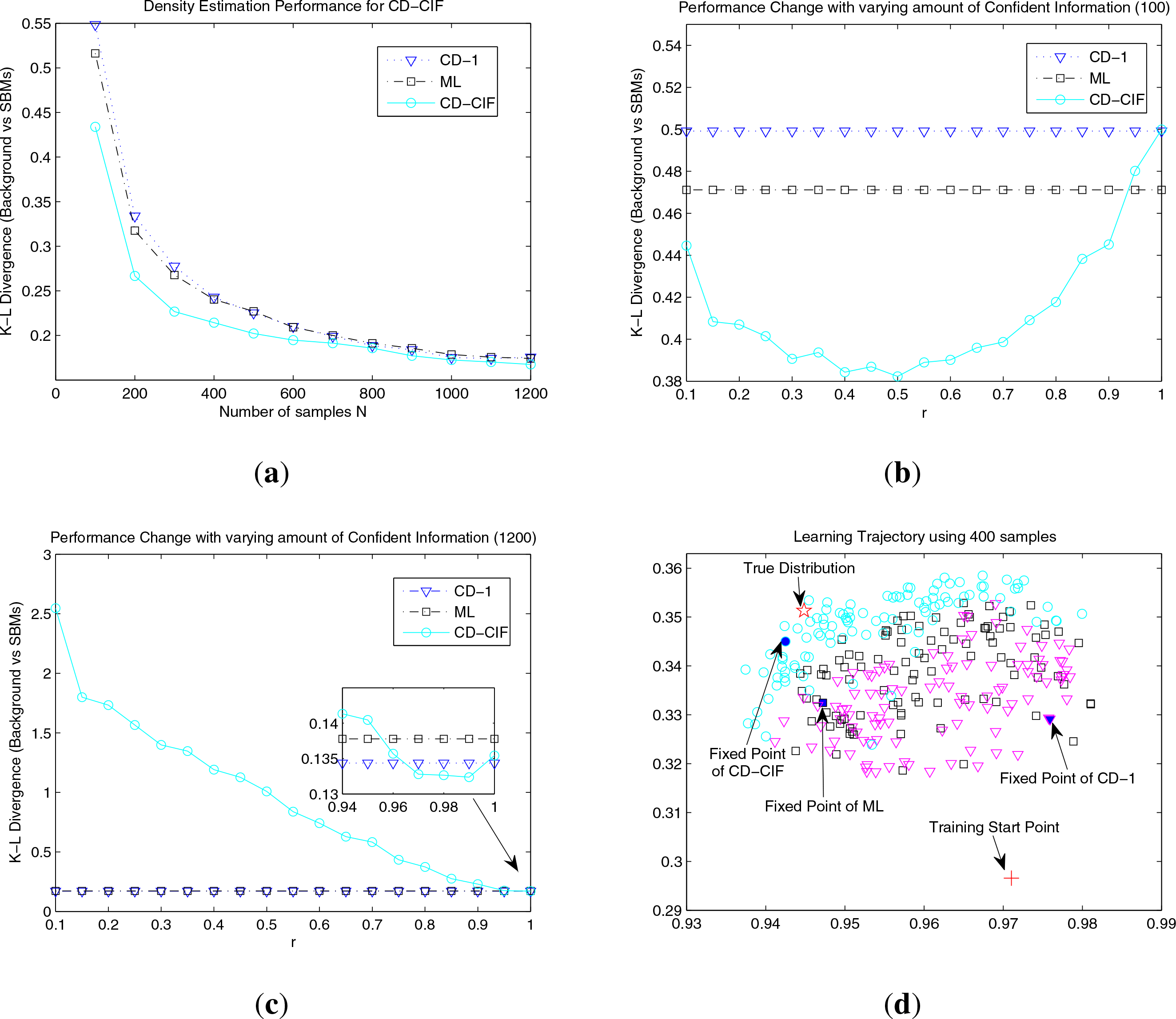
In this section, we empirically investigate our justifications for the CIF principle, especially how the sample-specific CIF-based CD learning (see Section 5) works in the context of density estimation.

Experimental Setup and Evaluation Metric: We utilize the random distribution uniformly generated from the open probability simplex over 10 variables as underlying distributions, whose samples size N may vary. Three learning algorithms are investigated: ML, CD-1 and our CD-CIF. K-L divergence is used to evaluate the goodness-of-fit of the SBM’s trained by various algorithms. For sample size N, we run 100 instances (20 (randomly generated distributions) × 5 (randomly running)) and report the averaged K-L divergences. Note that we focus on the case that the variable number is relatively small (n =10) in order to analytically evaluate the K-L divergence and give a detailed study on algorithms. Changing the number of variables only offers a trivial influence for the experimental results, since we obtained qualitatively similar observations on various variable numbers (not reported here).

Automatically Adjusting r for Different Sample Sizes: The Fisher information is additive for i.i.d. sampling. When sample sizes change, it is natural to require that the total amount of Fisher information contained in all tailored parameters is steady. Hence, we have α = (1 − r)N, where α indicates the amount of Fisher information and becomes a constant when the learning model and the underlying distribution family are given. It turns out that we can first identify α using the optimal r w.r.t several distributions generated from the underlying distribution family and then determine the optimal r’s for various sample sizes using r = 1 − α/N. In our experiments, we set α = 35.

Density Estimation Performance: The averaged K-L divergences between SBMs (learned by ML, CD-1 and CD-CIF with the r automatically determined) and the underlying distribution are shown in Figure 3a. In the case of relatively small samples (N ≤ 500) in Figure 3a, our CD-CIF method shows significant improvements over ML (from 10.3% to 16.0%) and CD-1 (from 11.0% to 21.0%). This is because we could not expect to have reliable identifications for all model parameters from insufficient samples, and hence, CD-CIF gains its advantages by using parameters that could be confidently estimated. This result is consistent with our previous theoretical insight that Fisher information gives a reasonable guidance for parametric reduction via the confidence criterion. As the sample size increases (N ≥ 600), CD-CIF, ML and CD-1 tend to have similar performances, since, with relatively large samples, most model parameters can be reasonably estimated, hence the effect of parameter reduction using CIF gradually becomes marginal. In Figure 3b and Figure 3c, we show how sample size affects the interval of r. For N = 100, CD-CIF achieves significantly better performances for a wide range of r. While, for N =1, 200, CD-CIF can only marginally outperform baselines for a narrow range of r.

Effects on Learning Trajectory: We use the 2D visualizing technology SNE [20] to investigate learning trajectories and dynamical behaviors of three comparative algorithms. We start three methods with the same parameter initialization. Then, each intermediate state is represented by a 55-dimensional vector formed by its current parameter values. From Figure 3d, we can see that: (1) In the final 100 steps, the three methods seem to end up staying in different regions of the parameter space, and CD-CIF confines the parameter in a relatively thinner region compared to ML and CD-1; (2) The true distribution is usually located on the side of CD-CIF, indicating its potential for converging to the optimal solution. Note that the above claims are based on general observations, and Figure 3d is shown as an illustration. Hence, we may conclude that CD-CIF regularizes the learning trajectories in a desired region of the parameter space using the sample-specific CIF.

6. Conclusions

Different from the traditional EPI, the CIF principle proposed in this paper aims at finding a way to derive computational models for universal cognitive systems by a dimensionality reduction approach in parameter spaces: specifically, by preserving the confident parameters and reducing the less confident parameters. In principle, the confidence of parameters should be assessed according to their contributions to the expected information distance between the ideal distribution and its fluctuated observations. This is called the distance-based CIF. For some coordinated systems, e.g., the mixed-coordinate system [ζ]_l, the confidence of a parameter can also be directly evaluated by its Fisher information, which establishes a connection with the inverse variance of any unbiased estimate for the parameter via the Cramér–Rao bound. This is called the information-based CIF. The criterion of information-based CIF (i.e., Fisher information) can be seen as an approximation to distance-based CIF, since it neglects the influence of parameter scaling to the expected information distance. However, considering the standard mixed-coordinates [ζ]_l for the manifold of multivariate binary distributions, it turns out that both distance-based CIF and information-based CIF entail the same optimal submanifold M.

The CIF provides a strategy for the derivation of probabilistic models. The SBM is a specific example in this regard. It has been theoretically shown that the SBM can achieve a reliable representation in parameter spaces by using the CIF principle.

The CIF principle can also be used to modify existing SBM training algorithms by incorporating data information, such as CD-CIF. One interesting result shown in our experiments is that: although CD-CIF is a biased algorithm, it could significantly outperform ML when the sample is insufficient. This suggests that CIF gives us a reasonable criterion for utilizing confident information from the underlying data, while ML lacks a mechanism to do so.

In the future, we will further develop the formal justification of CIF w.r.t various contexts (e.g., distribution families or models).