Network Decomposition and Complexity Measures: An Information Geometrical Approach


Sony Computer Science Laboratories, inc. Takanawa muse bldg. 3F, 3-14-13, Higashi Gotanda, Shinagawa-ku, Tokyo 141-0022, Japan
Entropy 2014, 16(7), 4132-4167; https://doi.org/10.3390/e16074132
Submission received: 28 March 2014
/
Revised: 24 June 2014
/
Accepted: 14 July 2014
/
Published: 23 July 2014
(This article belongs to the Special Issue Information Geometry)
Abstract
:We consider the graph representation of the stochastic model with n binary variables, and develop an information theoretical framework to measure the degree of statistical association existing between subsystems as well as the ones represented by each edge of the graph representation. Besides, we consider the novel measures of complexity with respect to the system decompositionability, by introducing the geometric product of Kullback–Leibler (KL-) divergence. The novel complexity measures satisfy the boundary condition of vanishing at the limit of completely random and ordered state, and also with the existence of independent subsystem of any size. Such complexity measures based on the geometric means are relevant to the heterogeneity of dependencies between subsystems, and the amount of information propagation shared entirely in the system.

1. Introduction
Complex systems sciences emphasize on the importance of non-linear interactions that can not be easily approximated linearly. In other word, the degrees of non-linear interactions are the source of complexity. The classical reductionism approach generally decomposes a system into its components with linear interactions, and tries to evaluate whether the whole property of the system can still be reproduced. If this decomposition of a system destroys too much information to reproduce the system’s whole property, the plausibility of such reductionism is lost. Inversely, if we can evaluate how much information is ignored by the decomposition, we can assume how much complexity of the whole system is lost. This gives us a way to measure the complexity of a system with respect to the system decomposition.
In stochastic systems described as a set of joint distributions, the interaction can basically be expressed as the statistical association between the variables. The simplest reductionism approach is to separate the whole system into some subsets of variables, and assume the independence between them. If such decomposition does not affect the system’s property, the isolated subsystem is independent from the rest. On the other hand, if the decomposition loses too much information, then the subsystem is inside of a larger subsystem with strong internal dependencies and can not be easily separated.
The stochastic models have often been represented with the use of graph representation, and treated with the name of complex network [1–3]. Generally, the nodes represent the variables and the weights on the edges are the statistical association between them. However, if we consider the information contained in the different orders of dependencies among variables, the graph with a single kind of edges is not sufficient to express the whole information of the system [4]. An edge of a graph with n nodes contains the information of statistical association up to the n-th order dependencies among n variables. If we try to decompose the system independently by cutting these information, we have to consider what it means to cut the edge of the graph from the information theoretical point of view.
Indeed, analysis on the degree of dependencies existing between variables derived many definition of complexity in stochastic model [5], which have been mostly studied with information theoretical perspective. Beginning with seminal works of Lempel and Ziv (e.g., [6]), computation-oriented definition of complexity takes deterministic formalization and measures the necessary information to reproduce a given symbolic sequence exactly, which is classified with the name of algorithmic complexity [7–9].
On the other hand, statistical approach to complexity, namely statistical complexity, assumes some stochastic model as theoretical basis, and refers to the structure of information source on it in measure-theoretic way [10–12].
One of the most classical statistical complexities is the mutual information between two stochastic variables, and its generalized form to measure dependence between n variables is proposed (e.g., [13]) and explored in relevance to statistical models and theories by several authors [14–16].
We should also recall that complexity is not necessary conditioned only by information theory, but rather motivated from the organization of living system such as brain activity. The TSE complexity shows further extension of generalized mutual information into biological context, where complexity exists as the heterogeneity between different system hierarchies [17]. These statistical complexities are all based on the boundary condition of vanishing at the limit of completely random and ordered state [18].
The complexity measure is usually the projection from system’s variables to one-dimensional quantity, which is composed to express the degree of characteristic that we define to be important in what means “complexity”. Since the complexity measure is always a many-to-one association, it has both aspects of compressing information to classify the system from simple to complex, and losing resolution of the system’s phase space. If the system has n variables, we generally need n independent complexity measures to completely characterize the system with real-value resolution. The problematics of defining a complexity measure is situated on the edge of balancing the information compression on system’s complexity with theoretical support, and the resolution of the system identification to be maintained high enough to avoid trivial classification. The latter criterion increases its importance as the system size becomes larger. The better complexity measure is therefore a set of indices, with as less number as possible, which characterizes major features related to the complexity of the system. In this sense, the ensemble of complexity measures is also analogous to the feature space of support vector machine. A non-trivial set of complexity measures need to be complementary to each other in parameter space for the possible best discrimination of different systems.
In this paper, we first consider the stochastic system with binary variables and theoretically develop a way to measure the information between subsystems, which is consistent to the information represented by the edges of the graph representation.
Next, we particularly focus on the generalized mutual information as a start point of the argument, and further consider to incorporate network heterogeneity into novel measures of complexity with respect to the system’s decompositionability. This approach will be revealed to be complementary to TSE complexity as the difference between arithmetic and geometric means of information.
2. System Decomposition
Let us consider the stochastic system with n binary variables x = (x1, ··· , xn) where xi ∈ {0, 1} (1 ≤ i ≤ n). We denote the joint distribution of x by p(x). We define the decomposition pdec(x) of p(x) into two subsystems
and
(n1 + n2 = n, y1 ∪ y2 = x, y1 ∩ y2 = ϕ) as follows:
where p(y1) and p(y2) are the joint distributions of y1 and y2, respectively. For simplicity, hereafter we denote the system decomposition using the smallest subscript of variables in each subsystem. For example, in case n = 4, y1 = (x1, x3) and y2 = (x2, x4), we describe the decomposed system pdec(x) as < 1212 >. The system decomposition means to cut all statistical association between the two subsystems, which is expressed as setting the independent relation between them.
We will further consider the Equation (1) in terms of the graph representation. We define the undirected graph Γ:= (V, E) of the system p(x), whose vertices V = {x1, ··· , xn} and edges E = V × V represent the variables and the statistical association, respectively. To express the system, we set the value of each vertex as the value of the corresponding variable, and the weight of each edge as the degree of dependency between the connected variables.
There is however a problem considering the representation with a single kind of edge. The statistical association among variables is not only between two variables, but can be independently defined among plural variables up to the n-th order. Therefore, the exact definition of the weight of the edges remains unclear. To clarify these problematics, we consider the hierarchical marginal distributions η as another coordinates of the system p(x) as follows:
where
and
Since the definition of η is a linear transformation of p(x), both coordinates have the degrees of freedom
.
The subcoordinates η1 are simply the set of marginal distributions of each variable. The subcoordinates ηk (1 < k ≤ n) include the statistical association among k variables, that can not be expressed with the coordinates less than the k-th order. This means that the different statistical associations exist independently in each order among the corresponding sets of the variables. The statistical association represented by the weight of a graph edge {xi, xj} is therefore the superposition of the different dependencies defined on every subset of x including xi and xj.
To measure the degree of statistical association in each order, the information geometry established the following setting [19]. We first define another coordinates θ =(θ1; θ2; ··· ; θn) that are the dual coordinates of η with respect to the Legendre transformation of the exponential family’s potential function ψ(θ) to its conjugate potential ϕ(η) as follows:
where
Note that η can be inversely derived from θ, following Legendre transformation between ϕ(η) and ψ(θ):
Using the coordinates θ, the system is described in the form of the exponential family as follows:
The information geometry revealed that the exponential family of probability distribution forms a manifold with a dual-flat structure. More precisely, the coordinates θ form a flat manifold with respect to the Fisher information matrix as the Riemannian metric, and α-connection with α = 1. Dually to θ, the coordinates η are flat with respect to the same metric but α-connection with α = −1. It is known that θ and η are orthogonal to each other with respect to the Fisher information matrix. This structure give us a way to decompose the degree of statistical association among variables into separated elements of arbitrary orders. We define the so-called k-cut mixture coordinates ζk as follows [14].
We also define the k-cut mixture coordinates
= (ηk−;0, ··· , 0) with no dependency above the k-th order. We denote the system specified with ζk and
as p(x,ζk) and p(x,), respectively.
Then the degree of the statistical association more than the k-th order in the system can be measured by the Kullback-Leibler (KL-) divergence D[p(x,ζ): p(x,)].
where D[· : ·] is the KL-divergence from the first system to the second one.
Here, the decomposition is performed according to the orders of statistical association, which does not spatially distinguish the vertices. If we define the weight of an edge {xi, xj} with the KL-divergence, the above k-cut coordinates ζk are not appropriate to measure the information represented in each edge. We need to set another mixture coordinates so that to separate only the existing information between xi and xj regardless of its order.
Let us return to the definition of the system decomposition and consider on the dual-flat coordinates θ and η.
Proposition 1. The independence between the two decomposed systems y1 = (
, ··· ,
) and y2 =(
, ···,
) can be expressed on the new coordinates ηdec as follows:
where s[··· ] is the ascending sort of the internal sequence.
Then the corresponding dual coordinates θdec take 0 elements as follows:
Proof. For simplicity, we show the cases of n = 2 and n = 3 for the first node separation.
For n = 2, the above defined ηdec for the system decomposition < 12 > give its dual coordinates θdec as follows:
which means the first and second node is independent.
For n = 3, the above defined ηdec for the system decomposition < 122 > give its dual coordinates θdec as follows:
which means the first node is independent from the other nodes.
The generalization is possible with the use of recurrence formula between system size n and n +1, according to the symmetry of the model and Legendre transformation between ηdec and θdec coordinates.
Numerical proof can be obtained by computing directly 0 elements of θdec from ηdec.
The definition of ηdec means to decompose the hierarchical marginal distributions η into the products of the subsystems’ marginal distributions, in case the subscripts traverse the two subsystems. Therefore, only the statistical associations between two subsystems are set to be independent, while the internal dependencies of each subsystem remain unchanged. This is analytically equivalent to compose another mixture coordinates ξ, namely the < ··· >-cut coordinates, with proper description of the system decomposition with < ··· >. The ξ consists of the η coordinates with the subscripts that do not traverse between the decomposed subsystems, and the θ coordinates whose subscripts traverse between them.
For simplicity, we only describe here the case n = 4 and the decomposition < 1133 > (the set of the first, second, and the third, fourth nodes each form a subsystem). The system p(x) is expressed with the < 1133 >-cut coordinates ξ as
The decomposed system with no statistical association between two subsystems have the following coordinates ξdec, which is, in any decomposition, equivalent to set all θ in ξ as 0:
This is analytically equivalent to the definition of the decomposition (13)–(14) in case of < 1133 >. Therefore, the KL-divergence D[p(x,ξ) : p(x,ξdec)] measures the information lost by the system decomposition. The following asymptotic agreement to χ2 test also holds.
Proposition 2.
where ♯θ(ξ) is the number of θ coordinates appearing in the ξ coordinates.
3. Edge Cutting
We further expand the concept of system decomposition to eventually quantify the total amount of information expressed by an edge of the graph. Let us consider to cut an edge {xi, xj} (1 ≤ i < j ≤ n) of the graph with n vertices. Hereafter we call this operation as the edge cutting i − j. In the same way as the system decomposition, the edge cutting corresponds to modify the η coordinates to produce ηec coordinates as follows:
and the rest of ηec remains the same as those of η.
The formation of ηec from η consists of replacing the k-th order elements (k ≥ 3) of η including both i and j in its subscripts, with the product of the k − 1-th order η in maximum subgraphs (k − 1 vertices) each including i or j. This means that all orders of statistical association including the variables xi and xj are set to be independent only between them. Other relations that do not include simultaneously xi and xj remain unchanged.
Certain combinations of edge cuttings coincide with system decompositions. For example, in case n = 4, the edge cuttings 1 − 2, 1 − 3, and 1 − 4 are equivalent to the system decomposition < 1222 >.
We define the i − j-cut mixture coordinates ξ for orthogonal decomposition of the statistical association represented by the edge {xi, xj}. Although actual calculation can be performed only with η coordinates, this generalization is necessary to have a geometrical definition of the orthogonality. For simplicity, we only describe the ξ in the case of n = 4:
where orthogonality between the elements of η and θ holds with respect to the Fisher information matrix.
Calculating the dual coordinates θec of ηec, we can define the coordinates ξec of the system after the edge cutting 1 − 2 as follows:
Note that the edge cutting can not be defined simply by setting the corresponding elements of θec as 0.
Then the KL-divergence D[p(x, ξ): p(x, ξec)] represent the total amount of information represented by the edge 1 − 2.
The following asymptotic agreement to χ2 test also holds:
Proposition 3.
We call this χ2 value or the KL-divergence itself as edge information of edge 1 − 2.
4. Generalized Mutual Information as Complexity with Respect to the Total System Decomposition
In previous sections, we have introduced a measure of complexity in terms of system decomposition, by measuring the KL-divergence between a given system and its independently decomposed subsystems. We consider here the total system decomposition, and measure the informational distance I between the system and the totally decomposed system where each element are independent.
where
This quantity is the generalization of mutual information, and is named in various ways such as generalized mutual information, integration, complexity, multi-information, etc. according to different authors. For simplicity, we call the I as “multi-information taking after [15]. This quantity can be interpreted as a measure of complexity that sums up the order-wise statistical association existing in each subset of components with information geometrical formalization [14]
For simplicity, we denote the multi-information I of n-dimensional stochastic binary variables as follows, using the notation of the system decomposition:
5. Rectangle-Bias Complexity
The multi-information contains some degrees of freedom in case n > 2. That is, we can define a set of distributions {p(x) I = const. } with different parameters but the same I value. This fact can be clearly explained with the use of information geometry. From the Pythagorean relation, we obtain the followings in case of n = 3:
Using these relations, we can schematically represent the decomposed systems on a circle diagram with diameter
. This representation is based on the analogous algebra between Pythagorean relation of KL-divergence, and that of Euclidian geometry where the circumferential angle of a semi-circular arc is always
.
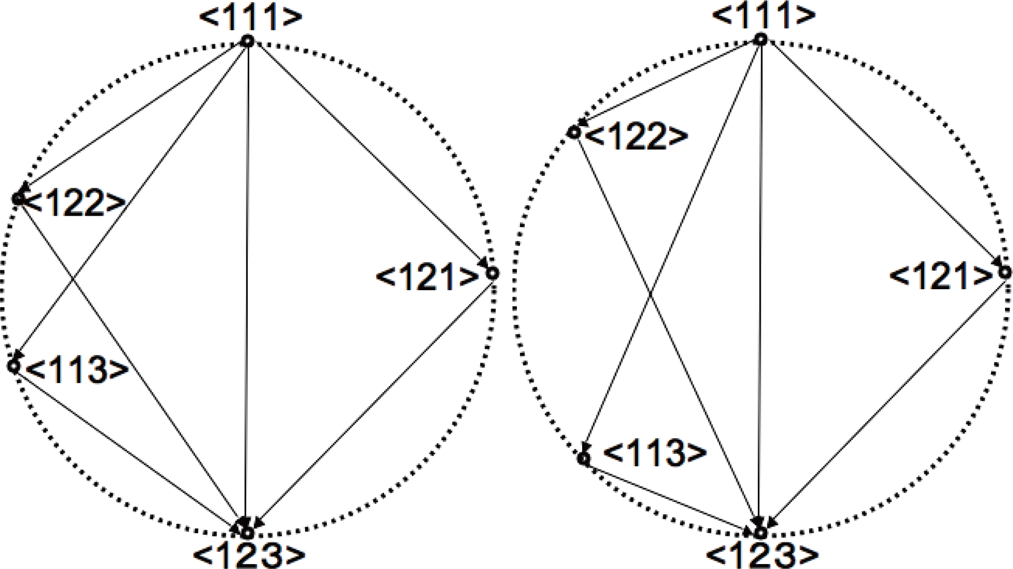
Figure 1 represents two different cases with the same I value in case n = 3. The distance between two systems in the same diagram corresponds to the square root value of KL-divergence between them. Clearly the left and right figures represent different dependencies between nodes, although they both have the same I value. Such geometrical variation is possible by the abundance of degree of freedom in dual coordinates compared to the given constraint. There exist 7 degrees of freedom in η or θ coordinates for n = 3, while the only constraint is the invariance of I value, which only reduce 1 degree of freedom. The remaining 6 degrees of freedom can then be deployed to produce geometrical variation in the circle diagram. As for considering system decomposition, the left figure is difficult to obtain decomposed systems without losing much information. While in the right figure there exists relatively easy decomposition < 122 >, which loses less information than any decomposition in the left figure. We call such degree of facility of decomposition with respect to the losing information as system decompositionability. In this sense, the left system is more complex although the 2 systems both have the same I value. Especially, in case D[< 111 >:< 122 >] = D[< 111 >:< 113 >] = D[< 111 >:< 121 >], the system does not have any easiest way of decomposition, and any isolation of a node loses significant amount of information.
To further incorporate such geometrical structure reflecting system decompositionability into a measure of complexity, we consider a mathematical way to distinguish between these two figures. Although the total sum of KL-divergence along the sequence of system decomposition is always identical to I by Pythagorean relation, their product can vary according to the geometrical composition in the circle diagram. This is analogous to the isoperimetric inequality of rectangle, where regular tetragon gives the maximum dimensions amongst constant perimeter rectangles.
We propose provisionary a new measure of complexity as follows, namely rectangle-bias complexity Cr:
where SD is the set of possible system decomposition in n binary variables, and |SD| is the element number of SD. For example, SD = {< 111 >, < 122 >, < 121 >, < 113 >,< 123 >} and |SD| = 5 for n = 3. This measure distinguishes between the two systems in Figure 1, and gives larger value for the left figure. It also gives maximum value in case D[< 111 >:< 122 >] = D[< 111 >:< 113 >] = D[< 111 >:< 121 >]. We propose provisionary a new measure of complexity as follows, namely rectangle-bias complexity Cr:
where SD is the set of possible system decomposition in n binary variables, and |SD| is the element number of SD. For example, SD = {< 111 >, < 122 >, < 121 >, < 113 >, < 123 >} and |SD| = 5 for n = 3. This measure distinguishes between the two systems in Figure 1, and gives larger value for the left figure. It also gives maximum value in case D[< 111 >:< 122 >] = D[< 111 >:< 113 >] = D[< 111 >:< 121 >].
6. Complementarity between Complexities Defined with Arithmetic and Geometric Means
We evaluate the possibility and the limit of rectangle-bias complexity Cr comparing with other proposed measures of complexity.
The Interests in measuring network heterogeneity have been developed toward the incorporation of multi-scale characteristics into complexity measures. The TSE complexity is motivated from the structure of the functional differentiation of brain activity, which measures the difference of neural integration between all sizes of subsystems and the whole system [17]. Biologically motivated TSE complexity is also investigated from theoretical point of view, to further attribute desirable property as an universal complexity measure independent of system size [20]. The hierarchical structure of the exponential family in information geometry also leads to the order-wise description of statistical association, which can be regarded as a multi-scale complexity measure [14]. The relation between the order-wise dependencies and the TSE complexity is theoretically investigated to establish the order-wise component correspondence between them [15].
These indices of network heterogeneity, however, all depend on the arithmetic mean of the component-wise information theoretical measure. We show that these arithmetic means still miss to measure certain modularity based on the statistical independence between subsystems.
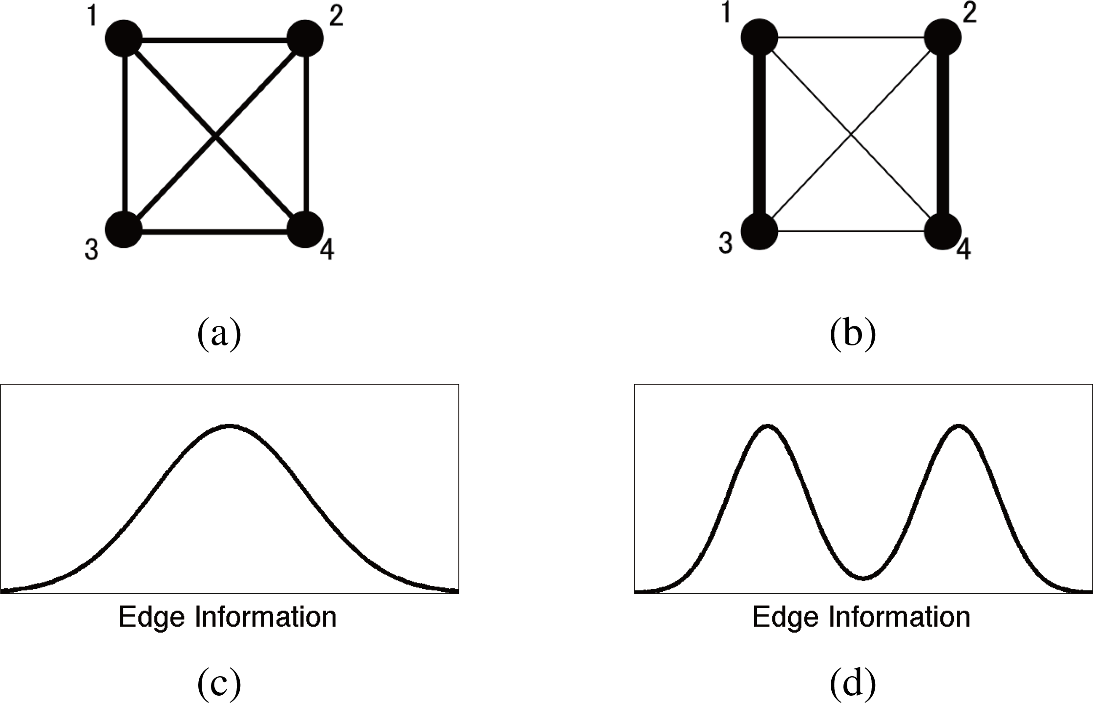
Figure 2 present the simplified cases where complexity measures with arithmetic means fail to distinguish. We consider the two systems with different heterogeneity but identical multi-information I. Here, the multi-information can not reflect the network heterogeneity. The TSE complexity and its information geometrical correspondence in [15] has a sensitivity to measure the network heterogeneity, but since the arithmetic mean is taken over all subsystems, they do not distinguish the component-wise break of symmetry between different scales. The renormalized TSE complexity with respect to the multi-information I still has the same insensitivity. Even by incorporating the information of each subsystem scale, the arithmetic mean can balance out between the scale-wise variations, and a large range of the heterogeneity in different scale can realize the same value of these complexities. For the application in neuroscience, the assumption of a model with simple parametric heterogeneity and the comparison of TSE complexity between different I values alleviate this limitation [17].
In contrast to complexities with arithmetic mean, the rectangle-bias complexity Cr is related to the geometrical mean. The Cr can distinguish the two systems in Figure 2, giving relatively high Cr value to the left system and low value to the right one.
This does not mean, however, that the Cr has a finer resolution than other complexity measures. The constant conditions of complexity measures are the constraints on
degrees of freedom in model parameter space, which define different geometrical composition of corresponding submanifolds. We basically need
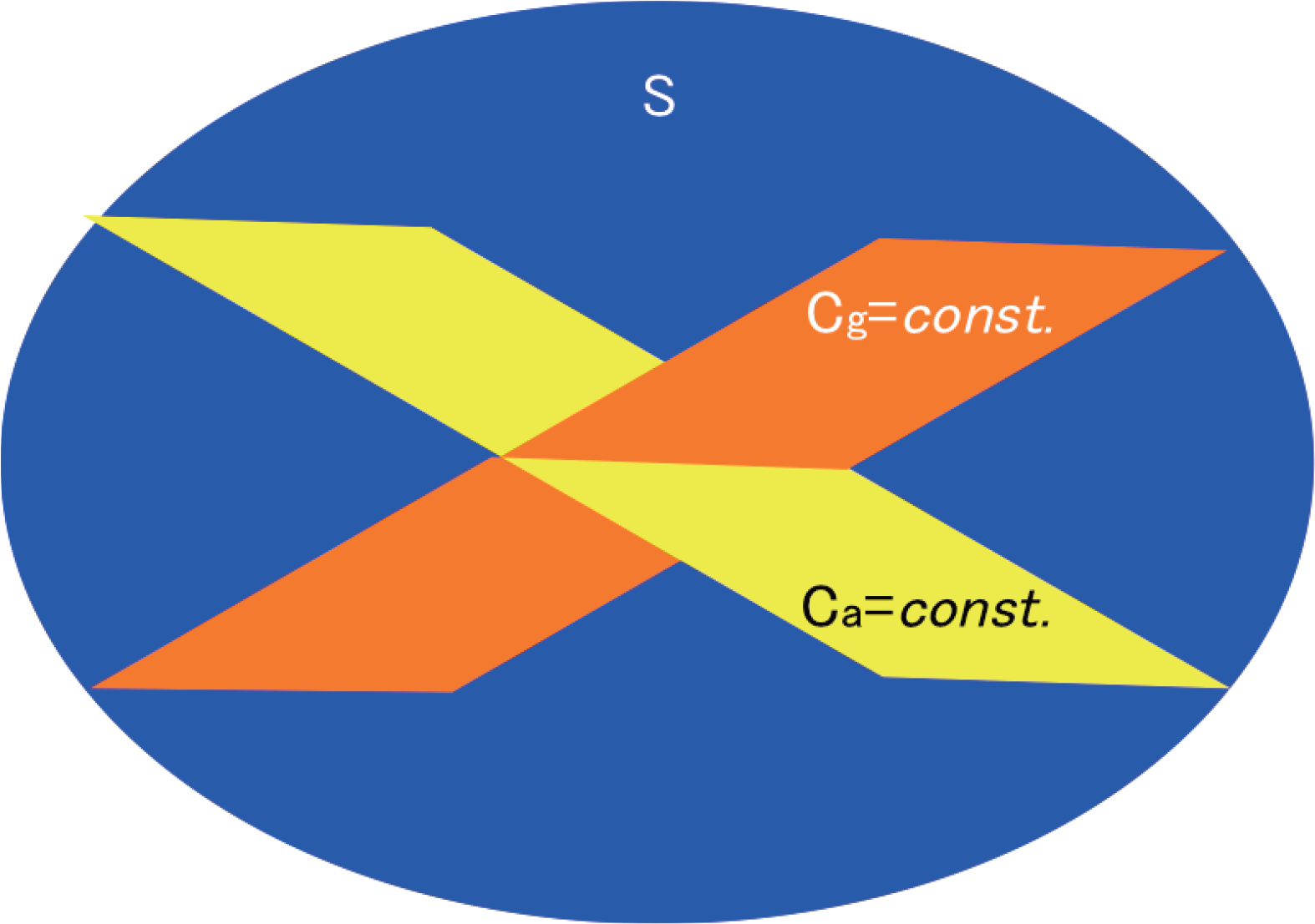
independent measures to assure the real-value resolution of network feature characterization. Complexities with arithmetic and geometric means are just giving complementary information on network heterogeneity, or different constant-complexity submanifolds structure in statistical manifold as depicted in Figure 3. Therefore, it is also possible to construct a class of systems that has identical I and Cr values but different TSE complexity. Complexity measures should be utilized in combination, with respect to the non-linear separation capacity of network features of interest.
7. Cuboid-Bias Complexity with Respect to System Decompositionability
We consider the expansion of Cr into general system size n. The n ≥ 4 situation is different from n = 3 and less in the existence of a hierarchical structure between system decompositions.
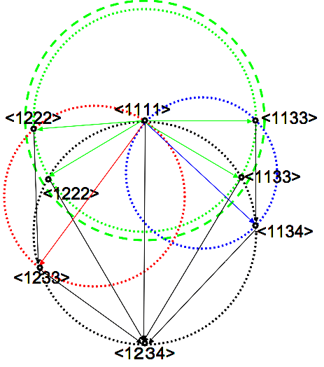
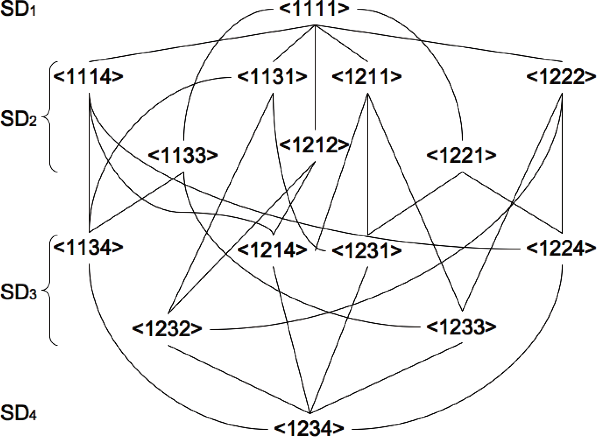
Figure 4 shows the hierarchy of the system decompositions in case n = 4. Such hierarchical structure between system decompositions is not homogeneous with respect to the subsystems number, and depends on the isomorphic types of decomposed systems. This fact produces certain difference of meaning in complexity between each KL-divergences when considering the system decompositionability.
A simple example in 4 nodes network is shown in Figure 5.
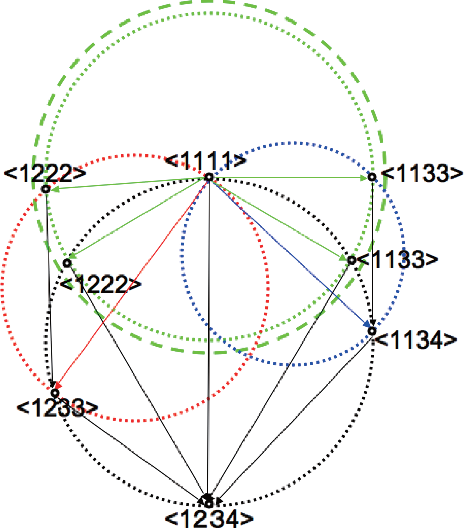
We consider the modification of 2 KL-divergences in the figure, D[< 1111 >:< 1222 >] and D[< 1111 >:< 1133 >] from the diameter of green dotted circle to the dashed one.
The joint distribution P (x1, x2, x3, x4) of a discrete distribution with 4 binary variables (x1, x2, x3, x4) (x1, x2, x3, x4 ∈{0, 1}) have 24 −1 = 15 parameters, which define the dual-flat coordinates of statistical manifold in information geometry.
On the other hand, the possible system decompositions exist as the followings in n = 4:
Since the number of possible system decompositions is 15, and each is associated with the modification of different sets of P (x1, x2, x3, x4) parameters, the system decompositions and KL-divergences between them can be defined independently. This also holds even under the constant condition of I value or other complexity measures except the ones imposing dependency between system decompositions.
This means that we can independently modify the diameter of green dotted circle in Figure 5, without changing the diameters of the red and blue circles, which define the system decompositions < 1233 > and < 1134 > in the sub-hierarchy of < 1222 > and < 1133 >, respectively. Other KL-divergences can also be maintained as given constant values for the same reason.
The rectangle-biased complexity Cr increases its value with such modification, but does not reflect the heterogeneity of KL-divergences according to the hierarchy of system decompositions. If we consider the system decompositionability as the mean facility to decompose the given system into its finest components with respect to the “all” possible system decompositions, such hierarchical difference also has a meaning in the definition of complexity.
The effect of modifying the diameter of the green dotted circle is different between the decomposition sequences < 1111 >→< 1222 >→< 1233 >→< 1234 > and < 1111 >→< 1133 > →< 1134 >→< 1234 >. The decrease of the KL-divergence D[< 1222 >:< 1233 >] is less than D[< 1133 >:< 1134 >] since the diameter of the red dotted circle is larger than the blue one in Figure 5. This means that the effect of changing the same amount of KL-divergences in D[< 1111 >:< 1222 >] and D[< 1111 >:< 1133 >] produces larger effect on the sequence < 1111 >→< 1133 >→< 1134 >→< 1234 > than < 1111 >→< 1222 >→< 1233 >→< 1234 >, if compared at the sequence level. The rectangle-biased complexity Cr does not reflect such characteristics since it does not distinguish between the hierarchical structure between the diameters of the green, red and blue dotted circles.
To incorporate such hierarchical effect in a complexity measure with geometric mean, we have the natural expansion of the rectangle-biased complexity Cr as the cuboid-bias complexity Cc, which is defined as follows:
where Seq represents the possible sequences of hierarchical system decompositions as follows:
The elements SDi(is) of Seq corresponds to the system decomposition, which is aligned according to the hierarchy with the following algorithmic procedure (based on [15]):
- (1)
- Initialization: Set the initial sets of system decomposition of all sequences in Seq as the whole system SD1(is):=< 111 ··· 1 > (1 ≤ is ≤ |Seq|).
- (2)
- Step i → i +1: If the system decomposition is the total system decomposition (SDi(is):=< 123 ··· n>), then stop. Otherwise, choose a non-decomposed subsystem SSi(is) of the system decomposition SDi(is), and further divide it into two independent subsystems and different for each is. SDi+1(is) is then defined as a system decomposition of total system that further separates independently subsystems and , in addition to the previous decomposition SDi(is).
- (3)
- Go to the next step i +1 → i +2.
The value of |Seq| corresponds to the number of different sequences generated by this algorithm. For example, |Seq| = 3 and |Seq| = 18 holds for n = 3 and n = 4, respectively. The general analytical form |Seq|n of |Seq| with system size n is obtained as the following recurrence formula:
where ⌊ · ⌋ is a floor function and with formal definition of |Seq|1 := 1.
The products of KL-divergences according to the hierarchical sequences of system decompositions in Equation (32) is related to the volume of n − 1-dimensional cuboids in the circle diagram. An example in case of n = 4 is presented in Figure 5, where two cuboids with 3 orthogonal edges of the different decomposition sequences < 1111 >→< 1222 >→< 1233 >→< 1234 > and < 1111 >→< 1133 >→< 1134 >→< 1234 > are depicted, whose cuboid volumes are
and
respectively.
In the same way as Cr, we took in the definition of Cc the arithmetic average of cuboid volumes so that to renormalize the combinatorial increase of the decomposition paths (|Seq|) according to the system size n.
Note that on the other hand we did not renormalize the rectangle-bias complexity Cr and the cuboid-bias complexity Cc by taking the exact geometrical mean of each product of KL-divergences such as
. This is for further accessibility to theoretical analysis such as variational method (see “Further Consideration” section), and does not change qualitative behavior of Cr and Cc since the power root is a monotonically increasing function. This treatment can be interpreted as taking the (n − 1)-th power of the geometric means for the hierarchical sequences of KL-divergences.
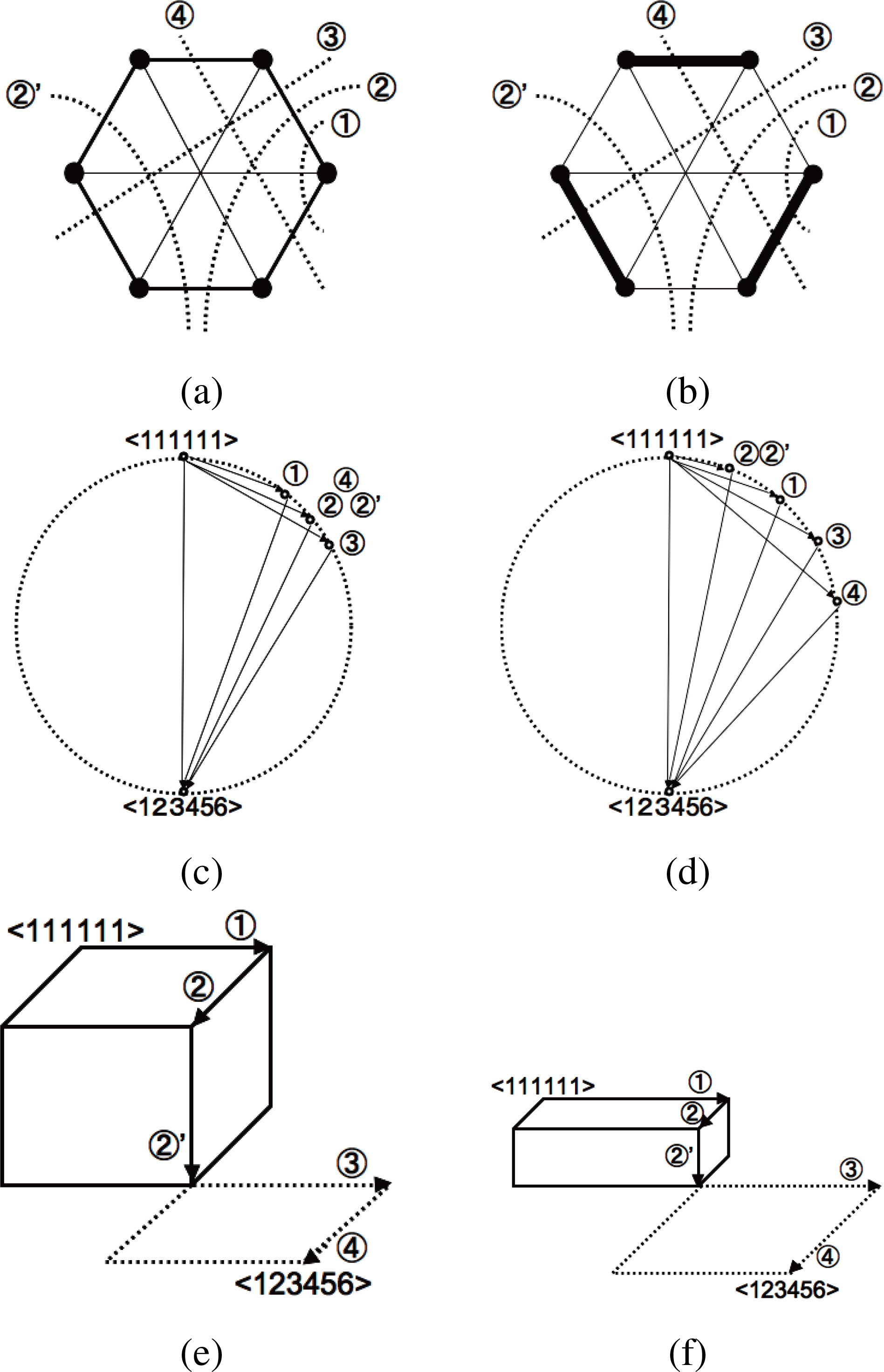
A more comprehensive example on the utility of the cuboid-bias complexity Cc with respect to the rectangle-biased one Cr is shown in Figure 6. We consider the 6 nodes networks (n = 6) with the same I and Cr values but different heterogeneity. The system in the top left figure has a circularly connected structure with medium intensity, while that of the top right figure has strongly connected 3 subsystems. These systems have qualitatively five different ways of system decomposition that are the basic generators of all hierarchical sequences Seq = {SD1(is) →··· → SD5(is)|1 ≤ is ≤ |Seq|} for these networks. The five basial system decompositions are shown with the number ①, ②, ②′, ③ and ④ in top figures.
The circle diagrams of these systems are depicted in the middle figures. To suppose the same constant value of Cr in both systems, the following condition is satisfied in the middle right figure: D[< 111111 >: ②] < D[< 111111 >: ①in Middle Left figure] < D[< 111111 >: ①] < D[< 111111 >: ②in Middle Left figure] <D[< 111111 >: ③] <D[< 111111 >: ④]. Furthermore, the total surface of right triangles sharing the circle diameter as hypotenuse in the middle left and the middle right figures are conditioned to be identical, therefore the rectangle-bias complexity Cr fails to distinguish.
On the other hand, under the same condition, the cuboid-bias complexity Cc distinguishes between these two systems and gives higher value to the left one. The volume of 5-dimensional cuboids of the decomposition sequence
are schematically shown in the bottom figures, maintaining the quantitative difference between KL-divergences. Since the multi-information I is identical between the two systems, so is the values of KL-divergence D[< 111111 >:< 123456 >], which is the sum of the KL-divergences along the sequence
from the Pythagorean theorem. This means that the inequality between the cuboid volumes can be represented as the isoperimetric inequality of high-dimensional cuboid. As a consequence, the left system has quantitatively higher value of Cc than the right one. The cuboid-bias complexity Cc is also sensitive to such heterogeneity.
8. Regularized Cuboid-Bias Complexity with Respect to Generalized Mutual Information
We further consider the geometrical composition of system decompositions in the circle diagram and insist the necessity of renormalizing the cuboid-bias complexity Cc with the multi-information I, which gives another measure of complexity namely “regularized cuboid-bias complexity.”
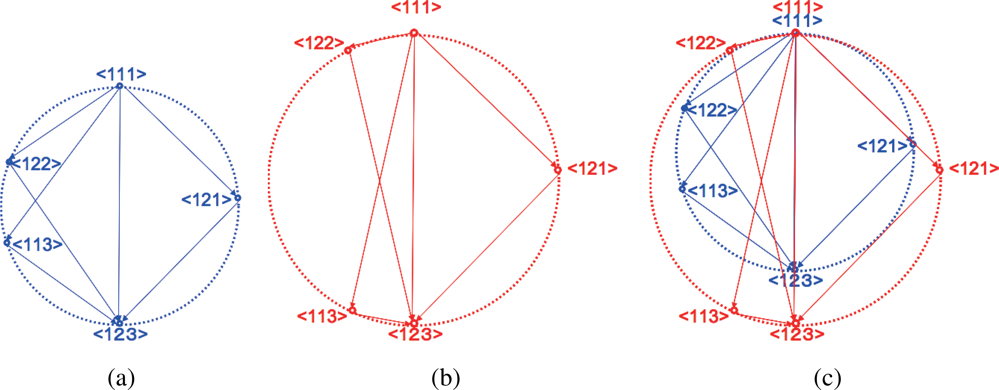
We consider the situation in actual data where the multi-information I varies. Figure 7 shows the n = 3 cases where the Cc fails to distinguish. Both the blue and red systems are supposed to have the same Cc value by adjusting the red system to have relatively smaller values of KL-divergences D[< 111 >:< 122 >] and D[< 113 >:< 123 >] than the blue one. Such conditioning is possible since the KL-divergences are independent parameters with each other.
Although the Cc value is identical, the two systems have different geometrical composition of system decompositions in the circle diagram. The red system has relatively easier way of decomposition < 111 >→< 122 > if renormalized with the total system decomposition < 111 >→< 123 >. This relative decompositionability with respect to the renormalization with the multi-information I can be clearly understood by superimposing the circle diagram of the two systems and comparing the angles between each and total decomposition paths (bottom figure). The red system has larger angle between the decomposition paths < 111 >→< 122 > and < 111 >→< 123 > than any others in the blue system, which represents the relative facility of the decomposition under renormalization with I. In this term, the paths < 111 >→< 121 > in the red and blue system do not change its relative facility, and the paths < 111 >→< 113 > are easier in the blue system.
To express the system decompositionability based on these geometrical compositions in a comprehensive manner, we define the regularized cuboid-bias complexity as follows:
The red system then has quantitatively smaller
value than the blue system in Figure 7.
9. Modular Complexity with Respect to the Easiest System Decomposition Path
We have considered so far the system decompositionability with respect to the all possible decomposition sequences. This was also a way to avoid the local fluctuation of the network heterogeneity to be reflected in some specific decomposition paths. On the other hand, the easiest decomposition is particularly important when considering the modularity of the system. If there exists hierarchical structure of modularity in different scales with different coherence of the system, the KL-divergence and the sequence of the easiest decomposition gives much information.
Figure 8 schematically shows a typical example where there exist two levels of modularity. Such structure with different scales of statistical coherence appears as functional segregation in neural systems [17], and is expected to be observed widely in complex systems.
The hierarchical topology of the easiest decomposition path reflects these structures. For example, in the system of Figure 8, the decompositions between < 1 1 ··· 1 > and < 1 1 1 1 5 5 5 5 9 9 9 9 1 3 1 3 1 3 1 3 > are easier than those inside of the 4-node subsystems. The values of KL-divergence also reflect the hierarchy, giving relatively low values for the decomposition between the 4-node subsystems, and high values inside of them. By examining the shortest decomposition path and associated KL-divergences in possible Seq, one can project the hierarchical structure of the modularity existing in the system.
For this reason, we define the modular complexity Cm as follows, which is the shortest path component of the cuboid-bias complexity Cc:
where the index imin of the sequence SD1(imin) → SD2(imin) → ··· → SDn(imin) is chosen as follows:
where
which gives eventually
This means that beginning from the undecomposed state < 11 ··· 1 >, we continue to choose the shortest decomposition path in the next hierarchy of system decomposition. The minimization of the path length is guaranteed by the sequential minimization since the geometric mean of isometric path division is bounded below by its minimum component. imin is unique if the system is completely heterogenous (i.e., D[SD1(ik): SD2(ik)] ≠ D[SD1(il) : SD2(il)], 1 ≤ ik <il ≤ |Seq|), otherwise plural decomposition paths that give the same Cm value are possible according to the homogeneity of the system. Besides its value, the modular complexity Cm should be utilized with the sequence information of the shortest decomposition path to evaluate the modularity structure of a system.
The cases where Cm are identical but Cc are different can be composed by varying the system decompositions other than in the shortest path SD1(imin) → SD2(imin) →··· → SDn(imin) without modifying the index imin. There exist also inverse examples with identical Cc and different Cm, due to the complementarity between Cm and Cc.
We finally define the regularized modular complexity as follows, for the same reason as defining
from Cc;
Proposition 4. The cuboid-bias complexities Cc and are bounded by the modular complexities Cm and respectively:
And they coincide at the maximum values under the given multi-information I:
These relations (43)–(46) are numerically shown in the “Numerical Comparison” section. The superiority of the modular complexities is due to the hierarchical dependency of KL-divergence value in decomposition paths. In the shortest decomposition path defining modular complexities, the easier system decomposition relatively increase its value since they incorporate more number of edge cutting. Since we eventually cut all edges to obtain < 12 ··· n > at the end of the decomposition sequence, collecting the edges with relatively weak edge information and cutting them together augment the value of the product of KL-divergences. The modular complexities are then the maximum value components among the possible decomposition paths calculated in cuboid-bias complexities:
The difference between the cuboid-bias complexities and the modular complexities is an index of the geometrical variation of decomposed systems in the circle graph, which reflects the fluctuation of the sequence-wise system decompositionability. If the variation of the system decompositionability for each system decomposition is large, accordingly the modular complexities tend to give higher values than the cuboid-bias complexities.
10. Numerical Comparison
We numerically investigate the complementarity between the proposed complexities, Cc,
, Cm, and
. Since the minimum node number giving non-trivial meaning to these measures is n = 4, the corresponding dimension of parameter space is
. The constant-complexity submanifolds are therefore difficult to visualize due to the high dimensionality. For simplicity, we focus on the 2-dimensional subspace of this parameter space whose first axis ranging from random to maximum dependencies of the system, and the second one representing the system decompositionability of < 1133 >.
For this purpose, we introduce the following parameters α and β (0 ≤ α, β ≤ 1) in the η-coordinates of the discrete distribution with 4-dimensional binary stochastic variable:
Where α represents the degree of statistical association from random (α = 0) to maximum (α = 1), and β control the system decompositionability of < 1133 >. If β = 1, the system has the maximum KL-divergence D[< 1111 >:< 1133 >] under the constraint of α parameter, and β = 0 gives D[< 1111 >:< 1133 >] = 0.
∊ is the minimum value of the joint distribution of 4-dimensional variable, which is defined to be more than 0 to avoid singularity in the dual-flat coordinates of statistical manifold. ∊ = 1.0 × 10⁻¹⁰ and η0 = 0.5 was chosen for the calculation.
The system with maximum statistical association under given η0 corresponds to the α = β = 1 condition in given parameters, whose η-coordinates become as follows:
On the other hand, the totally decomposed system corresponds to the α = 0 condition, and the η-coordinates are:
Note that the completely deterministic case η0 = 1.0 and α = β = 1 gives I = 0.
The intuitive meaning of these parameters α and β are also schematically depicted in Figure 9 bottom right.
Figure 10 shows the landscape of the proposed complexities on the α−β plane. Their contour plots are depicted in Figure 9. The proposed complexities each differs from others in almost everywhere points on α−β plane except at the intersection lines. Therefore, these measures serve as the independent features of the system, each has its specific meaning with respect to the system decompositionability. The α−β plane shows a section of the actual structure of the complementarity expressed in Figure 3 between the proposed complexity measures.
The relations between the cuboid-bias complexities and modular complexities in Equations (43)–(46) are also numerically confirmed. The modular complexities are superior than the corresponding cuboid-bias complexities, and coincide at the parameter α = β = 1 giving maximum values and dependencies in this parameterization.
In general case without the parameterization with α, β and η0, the boundary conditions of Cc,
, Cm and
include that of the multi-information I, which vanish at the completely random or ordered state. This is common to other complexity measures such as the LMC complexity, and fit to the basic intuition on the concept of complexity situated equivalently far from the completely predictable and disordered states [21,22].
The proposed complexities further incorporate boundary conditions that vanish with the existence of a completely independent subsystem of any size. This means that the Cc,
, Cm and
of a system become 0 if we add another independent variable. This property does not reflect the intuition of complexity defined by the arithmetic average of statistical measures. The proposed complexity can better find its meaning in comparison to other complexity measures such as the multi-information I, and by interactively changing the system scale to avoid trivial results with small independent subsystem. For example, the proposed complexities could be utilized as the information criteria for the model selection problems, especially with an approximative modular structure based on the statistical independency of data between subsystems. We insist that the complementarity principle between plural complexity measures of different foundation is the key to understand the complexity in a comprehensive manner.
To characterize the property of Cc,
, Cm and
in relation to the diverse composition of each system decomposition, it is useful to consider the geometry of their contour structure, as compared in Figure 9. The contour can be formalized as Cc,
,Cm,
= const. for each complexity measure, and D[< 11 ··· 1 >: SDi(is)] = const. (1 ≤ i ≤ n−1, 1 ≤ is ≤ |Seq|) for each system decomposition. For that purpose, analysis with algebraic geometry can be considered as a prominent tool. Algebraic geometry investigates the geometrical property of polynomial equations [23]. The complexities Cc,
, Cm and
can be interpreted as polynomial functions by taking each system decomposition as novel coordinates, therefore directly accessible to algebraic geometry. However, if we want to investigate the contour of the complexities on the p parameter space, logarithmic function appears as the definition of KL-divergence, which is a transcendental function and outreach the analytical requirement of algebraic geometry. To introduce compatibility between the p parameter space of information geometry and algebraic geometry, it suffices to describe the model by replacing the logarithmic functions as another n variables such as q =log p, and reconsider the intersection between the result from algebraic geometry on the coordinates (p, q) and q =log p condition. The contour of Cc,
, Cm and
is also important to seek for the utility of these measures as a potential to interpret the dynamics of statistical association as geodesics.
11. Further Consideration
11.1. Pythagorean Relations in System Decomposition and Edge Cutting
We further look back at the system decomposition and edge cutting in terms of the Pythagorean relation between KL-divergences, which is based on the orthogonality between θ and η coordinates.
In system decomposition, the distribution of decomposed system is analytically obtained from the product of subsystems’ η coordinates, which is equivalent to set all θdec parameters as 0 in mixture coordinate ξdec. From the consistency of θdec parameters in ξdec being 0 in all system decompositions, we have the Pythagorean relation according to the inclusion relation of system decomposition. For example, the following holds:
The proof is in the same way as k-cut coordinates isolating k-tuple statistical association between variables [14].
On the other hand, the edge cutting previously defined using the product of remaining maximum cliques’ η coordinates does not coincides with the θec = 0 condition in mixture coordinates ξec. We have defined the ηec values of edge cutting based only on the orthogonal relation between η and θ coordinates, by generalizing the rule of system decomposition in ηec coordinates, and did not consider the Pythagorean relation between different edge cuttings.
It is then possible to define another way of edge cutting using θec = 0 condition in ξec. Indeed, in k-cut mixture coordinates, θk+ = 0 condition is derived from the independent condition of the variables in all orders, and k-tuple statistical association is measured by reestablishing the η parameters for the statistical association up to k − 1-tuple order. In the same way, we can set θdec = 0 condition for ξdec of a system decomposition, and reestablish edges with respect to the η parameters, except the one in focus for edge cutting.
As a simple example, consider the system decomposition < 1222 > and edge cutting 1 − 2 in 4-node graph. We have the mixture coordinate ξdec for the system decomposition as follows:
where all the rest of ξdec coordinates is equivalent to that of η coordinates.
We then consider the new way of edge cutting 1 − 2 by recovering the statistical association in edges 1 − 3 and 1 − 4 from system decomposition < 1222 >, orthogonally to that of edge 1 − 2. The new mixture coordinate ξEC changes to the following:
and the rest is equivalent to that of η coordinates.
This new ξEC is also compatible with k-cut coordinates formalization for its simple θEC = 0 conditions. To obtain ξEC for arbitrary edge cutting i − j, one should take θEC containing i and j in its subscript, set them to 0, and combine with η coordinates for the rest of the subscript. For plural edge cuttings i − j, ··· , k − l (1 ≤ i, j, k, l ≤ n), it suffices to take θEC containing i and j, ... , k and l in its subscript respectively, then set them to 0.
We finally obtain the Pythagorean relation between edge cuttings. Denoting the general edge cutting(s) coordinates as ξi−j,··· , k−l, the following holds for the example of system decomposition < 1222 >:
Despite the consistency with the dual structure between θ and η, we do not generally have analytical solution to determine ηEC values from θEC = 0 conditions. We should call for some numerical algorithm to solve θEC = 0 conditions with respect to ηEC values, which are in general high-degree simultaneous polynomials. Furthermore, numerical convergence of the solution has to be very strict, since tiny deviation from the conditions can become non-negligible by passing fractional function and logarithmic function of θ coordinates.
On the other hand, the previously defined edge cutting with ξec using the product between subgraphs’ η coordinates is analytically simple and does not need to consider the other edges’ recovery from system decomposition or independence hypothesis. We then chose the previous way of edge cutting for both calculability and clarity of the concept.
There have been many attempts to approximate complex network by low-dimensional system with the use of statistical physics and network theory. As a contemporary example, moment-closure approximation provides a various way to abstract essential dynamics e.g., in discrete adaptive network [24]. Although the approximation takes several theoretical assumptions such as random graph approximation, it is difficult to quantitatively reproduce the dynamics even in some simplest model. This is partly due to homogeneous treatment of statistics such as truncation into pair-wise order. The edge cutting can offer a complementary view on the evaluation of moment-closure approximations. Using orthogonal decomposition between edge information, one can evaluate which part of network link and which order of statistics contain essential information, which does not necessary conform to top-down theoretical treatment.
11.2. Complexity of the Systems with Continuous Phase Space
We have developed the concept of system decompositionability based on discrete binary variables. One can also apply the same principle to continuous variable.
For an ergodic map G : X → X in continuous space X, KS entropy h(μ, G) is defined as the maximum of entropy rate with respect to all possible system decomposition A, when the invariant measure μ exists:
where A is the disjoint decomposition of X that consists of non-trivial sets ai, whose total number is n(A), defined as
meaning the natural expansion of system decomposition into continuous space.
The entropy rate h(μ, G, A) in Equation (56) is defined as
according to the entropy H(μ, A) based on the decomposition A = {ai}
and the product C = A ∨ B as
In a more general case, topological entropy hT (G) is defined simply with the number of decomposed subsystem elements by preimages as follows, without requiring ergodicity, therefore neither the existence of invariant measure μ:
Topological entropy takes the maximum value of the possible preimage divisions, in order to measure the complexity in terms of the mixing degree of the orbits. For example, if the KS entropy is positive as h(μ, G) > 0, the dynamics of G on an invariant set of invariant measure μ is chaotic for almost everywhere initial conditions. As for the positive topological entropy hT (G) > 0, the dynamics of G contain chaotic orbits, but not necessary as attractive chaotic invariant set, since hT (G) ≥ h(μ, G) and the KS entropy can be negative.
Although these definitions are useful to characterize the existence of chaotic dynamics, the system decompositionability is another property representing different aspect of the system complexity. It is rather the matter of the existence of independent dynamics components, or the degree of orbit localization between arbitrary system decompositions. We propose the following “geometric topological entropy” hg(G) applying the same principle of taking geometric product between all hierarchical structure of the system decomposition A.
where σ(A) > 0 means to take all components of A having positive Lebesgue measure on X.
This gives 0 if the preimage of certain ai ∈A is ai itself, meaning there exist a subsystem ai whose range is invariant under G, closed by itself. The system X can be completely divided into ai and the rest. This corresponds to the existence of an independent subsystem in cuboid-bias and modular complexities. In case such independent components do not exist, it still reflects the degree of orbit localization for all possible system decompositions in multiplicative manner. The condition σ(A) > 0 is to avoid trivial case such as the existence of unstable limit cycle, whose Lebesgue measure is 0.
Typical example giving hg(G)= 0 is the function having independent ergodic components, such as the Chirikov-Taylor map with appropriate parameter [25].
12. Conclusions and Discussion
We have theoretically developed a framework to measure the degree of statistical association existing between subsystems as well as the ones represented by each edge of the graph representation. We then reconsidered the problem of how to define complexity measures in terms of the construction of non-linear feature space. We defined new type of complexity based on the geometrical product of KL-divergence representing the degree of system decompositionability. Different complexity measures as well as newly proposed ones are compared on a complementarity basis on statistical manifold.
Application of presented theory can encompass a large field of complex systems and data science, such as social network, genetic expression network, neural activities, ecological database, and any kind of complex networks with binary co-occurrence matrix data e.g., [26–29], databases: [30–34]. Continuous variables are also accessible by appropriate discretization of information source with e.g., entropy maximization principle.
In contrast to arithmetic mean of information over the whole system, geometric mean has not been investigated sufficiently in the analysis of complex network. However in different fields, theoretical ecology has already pointed out the importance of geometric mean when considering the long-term fitness of a species population in a randomly varying environment [35,36]. Long-term fitness refers to the ecological complexity of its survival strategy under large stochastic fluctuation. Here, we can find useful analogy between the growth rate of a population in ecology and the spatio-temporal propagation rate of information between subsystems in general. If we take an arbitrary subsystem and consider the amount of information it can exchange with all other subsystems, the proposed complexity measures with geometric mean reflect the minimum amount with amongst all possible other subsystems, which can not be distinguished with arithmetic mean. The propagation rate of a population in ecology and the information transmission in complex network hold mathematically analogous structure. In population ecology, the variance of growth rate is crucial to evaluate the long-term survival of the population. Even if the arithmetic mean of growth rate is high, large variance will lead to low geometric mean even with a small amount of exceptionally small fitness situation, which ecologically means extinction of an entire species. In stochastic network, the variance of system decompositionability is essential to evaluate the amount of information shared between subsystems, or information persistence in the entire network. Even the multi-information I is high, large heterogeneity of edge information can lead to informational isolation of certain subsystem, which means extinction of its information. If such subsystem is situated on the transmission pathway, information cannot propagate across these nodes. Therefore, the proposed complexity measures CC,
, Cm and
generally reflect the minimum amount of information propagation rate spread entirely on the system without exception of isolated division.
Some recent studies on adaptive network focus on the evolution of network topology in response to node activity, such as game-theoretic evolution of strategies [37], opinion dynamics on an evolving network [38], epidemic spreading on an adaptive network [39], etc. Analysis of coevolution network between variables and interactions can capture important dynamical feature of complex systems. In contrast to topological network analysis, the newly proposed complexity measures can complement its statistical dynamics analysis. In addition to the topological change of network model, (e.g., linking dynamics of game theory, opinion community network structure, contact network of epidemics transmission), one can evaluate the emerged statistical association between the variables that does not necessary coincide with the network topology. Interesting feature of non-linear dynamics is the unexpected correlation between distant variables, which is quantified as Tsallis entropy [40]. The complementary relation between concrete interaction and resulting statistical association can provide a twofold methodology to characterize the coevolutionary dynamics of adaptive network. Such strategy can promote integrated science from laboratory experiments to open-field in natura situation, where actual multi-scale problematics remain to be solved [41].
Arithmetic and geometric means can be integrated in a mutual formula called generalized mean [42]. Therefore, the proposed complexity measures with geometric mean of KL-divergence is an expansion of preexisting complexity measures with mixture coordinates. Table 1 summarizes the generalization of complexity measure in this article. Based on the k-cut coordinates ζ, the weighted sum of KL-divergence representing k-tuple order of statistical association derived complexity measures with (weighted) arithmetic mean such as multi-information I and TSE complexity. On the other hand, we showed that subsystem-wise correlation can also be isolated with the use of mixture coordinates, namely < ··· >-cut coordinates ξ. To quantify the heterogeneity of system decompositionability, we generally took a weighted geometric mean of KL-divergence in CC,
, Cm and
. Here, the shortest path selection of Cm and
, and regularization of
and
with respect to multi-information I can be interpreted as the weight function of geometric mean. This perspective brings a definition of a generalized class of complexity measures based on the mixture coordinates and generalized mean of KL-divergence. Information discrepancy can also be generalized from KL-divergence to Bregman divergence, providing access to the concept of multiple centroids in large stochastic data analysis such as image processing [43]. The blank columns of the Table 1 imply the possibility of other complexity measures in this class. For example, the weighted geometric mean of KL-divergence defined between k-cut coordinates is expected to yield complexity measures that are sensitive to the heterogeneity of correlation orders. The weighted arithmetic mean of KL-divergence defined between < ··· >-cut coordinates should be sensitive to the mean decompositionability of arbitrary subsystem. Since these measures take analytically different form on mixture coordinates and/or mean functions, their derivatives do not coincide, which give independent information of the system on the complementary basis on statistical manifold, as long as the number of complexity measures are inferior to the freedom degree of the system.
Acknowledgments
This study was partially supported by CNRS, the long term study abroad support program of the university of Tokyo, and the French government (Promotion Simone de Beauvoir).
Conflicts of Interest
The author declares no conflict of interest.
References
- Boccalettia, S.; Latorab, V.; Morenod, Y.; Chavezf, M.; Hwang, D.U. Complex Networks: Structure and Dynamics. Phys. Rep 2006, 424, 175–308. [Google Scholar]
- Strogatz, S.H. Exploring Complex Networks. Nature 2001, 410, 268–276. [Google Scholar]
- Wasserman, S.; Faust, K. Social Network Analysis; Cambridge University Press: Cambridge, UK, 1994. [Google Scholar]
- Funabashi, M.; Cointet, J.P.; Chavalarias, D. Complex Network. In Studies in Computational Intelligence; Springer: Berlin/Heidelberg, Germany, 2009; Volume 207, pp. 161–172. [Google Scholar]
- Badii, R.; Politi, A. Complexity: Hierarchical Structures and Scaling in Physics; Cambridge University Press: Cambridge, UK, 2008. [Google Scholar]
- Lempel, A.; Ziv, J. On the Complexity of Finite Sequences. IEEE Trans. Inf. Theory 1976, 22, 75–81. [Google Scholar]
- Li, M.; Vitanyi, P. Texts in Computer Science. In An Introduction to Kolmogorov Complexity and Its Applications, 2nd ed; Springer: Berlin/Heidelberg, Germany, 1997. [Google Scholar]
- Cover, T.M.; Thomas, J.A. Elements of Information Theory; Wiley: New York, NY, USA, 2006. [Google Scholar]
- Bennett, C. On the Nature and Origin of Complexity in Discrete, Homogeneous, Locally-Interacting Systems. Found. Phys 1986, 16, 585–592. [Google Scholar]
- Grassberger, P. Toward a Quantitative Theory of Self-Generated Complexity. Int. J. Theor. Phys 1986, 25, 907–938. [Google Scholar]
- Crutchfield, J.P.; Feldman, D.P. Regularities Unseen Randomness Observed: The Entropy Convergence Hierarchy. Chaos 2003, 15, 25–54. [Google Scholar]
- Crutchfield, J.P. Inferring Statistical Complexity. Phys. Rev. Lett 1989, 63, 105–108. [Google Scholar]
- Prichard, D.; Theiler, J. Generalized Redundancies for Time Series Analysis. Physica D 1995, 84, 476–493. [Google Scholar]
- Amari, S. Information Geometry on Hierarchy of Probability Distributions. IEEE Trans. Inf. Theory 2001, 47, 1701–1711. [Google Scholar]
- Ay, N.; Olbrich, E.; Bertschinger, N.; Jost, J. A Unifying Framework for Complexity Measures of Finite Systems; Report 06-08-028; Santa Fe Institute: Santa Fe, NM, USA, 2006. [Google Scholar]
- MacKay, R.S. Nonlinearity in Complexity Science. Nonlinearity 2008, 21, T273–T281. [Google Scholar]
- Tononi, G.; Sporns, O.; Edelman, M. A Measure for Brain Complexity: Relating Functional Segregation and Integration in the Nervous System. Proc. Natl. Acad. Sci. USA 1994, 91, 5033. [Google Scholar]
- Feldman, D.P.; Crutchfield, J.P. Measures of statistical complexity: Why? Phys. Lett. A 1998, 238, 244–252. [Google Scholar]
- Nakahara, H.; Amari, S. Information-Geometric Measure for Neural Spikes. Neural Comput 2002, 14, 2269–2316. [Google Scholar]
- Olbrich, E.; Bertschinger, N.; Ay, N.; Jost, J. How Should Complexity Scale with System Size? Eur. Phys. J. B 2008, 63, 407–415. [Google Scholar]
- Feldman, D.P.; Crutchfield, J.P. Measures of Statistical Complexity: Why? Phys. Lett. A 1998, 238, 244–252. [Google Scholar]
- Lopez-Ruiz, R.; Mancini, H.; Calbet, X. A Statistical Measure of Complexity. Phys. Lett. A 1995, 209, 321–326. [Google Scholar]
- Hodge, W.; Pedoe, D. Methods of Algebraic Geometry; Cambridge Mathematical Library, Cambridge University Press: Cambridge, UK, 1994; Volume 1–3. [Google Scholar]
- Demirel, G.; Vazquez, F.; Bohme, G.; Gross, T. Moment-closure Approximations for Discrete Adaptive Networks. Physica D 2014, 267, 68–80. [Google Scholar]
- Fraser, G. (Ed.) The New Physics for the Twenty-First Century; Cambridge University Press: Cambridge, UK, 2006; p. 335.
- Scott, J. Social Network Analysis: A Handbook; SAGE Publications Ltd.: London, UK, 2000. [Google Scholar]
- Geier, F.; Timmer, J.; Fleck, C. Reconstructing Gene-Regulatory Networks from Time Series, Knock-Out Data, and Prior Knowledge. BMC Syst. Biol 2007, 1. [Google Scholar] [CrossRef]
- Brown, E.N.; Kass, R.E.; Mitra, P.P. Multiple Neural Spike Train Data Analysis: State-of-the-Art and Future Challenges. Nat. Neurosci 2004, 7, 456–461. [Google Scholar]
- Yee, T.W. The Analysis of Binary Data in Quantitative Plant Ecology. Ph.D. Thesis, The University of Auckland, New Zealand. 1993. [Google Scholar]
- Stanford Large Network Dataset Collection. Available online: http://snap.stanford.edu/data/ (accessed on 19 July 2014).
- BioGRID. Available online: http://thebiogrid.org/ (accessed on 19 July 2014).
- Neuroscience Information Framework. Available online: http://www.neuinfo.org/ (accessed on 19 July 2014).
- Global Biodiversity Information Facility. Available online: http://www.gbif.org/ (accessed on 19 July 2014).
- UCI Network Data Repository. Available online: http://networkdata.ics.uci.edu/index.php (accessed on 19 July 2014).
- Lewontin, R.C.; Cohen, D. On Population Growth in a Randomly Varying Environment. Proc. Natl. Acad. Sci. USA 1969, 62, 1056–1060. [Google Scholar]
- Yoshimura, J.; Clark, C.W. Individual Adaptations in Stochastic Environments. Evol. Ecol 1969, 5, 173–192. [Google Scholar]
- Wu, B.; Zhou, D.; Wang, L. Evolutionary Dynamics on Stochastic Evolving Networks for Multiple-Strategy Games. Phys. Rev. E 2011, 84, 046111. [Google Scholar]
- Fu, F.; Wang, L. Coevolutionary Dynamics of Opinions and Networks: From Diversity to Uniformity. Phys. Rev. E 2008, 78, 016104. [Google Scholar]
- Gross, T.; D’Lima, C.J.D.; Blasius, B. Epidemic Dynamics on an Adaptive Network. Phys. Rev. Lett 2006, 96, 208701. [Google Scholar]
- Tsallis, C. Possible Generalization of Boltzmann-Gibbs Statistics. J. Stat. Phys 1988, 52, 479–487. [Google Scholar]
- Quintana-Murci, L.; Alcais, A.; Abel, L.; Casanova, J.L. Immunology in natura: Clinical, Epidemiological and Evolutionary Genetics of Infectious Diseases. Nat. Immunol 2007, 8, 1165–1171. [Google Scholar]
- Hardy, G.; Littlewood, J.; Polya, G. Inequalities; Cambridge University Press: Cambridge, UK, 1967; Chapter 3. [Google Scholar]
- Nielsen, F.; Nock, R. Sided and symmetrized Bregman centroids. IEEE Trans. Inf. Theory 2009, 55, 2882–2904. [Google Scholar]
Figure 1.
Circle diagrams of system decomposition in 3-node network. Both systems have the same value of multi-information I that is expressed as the identical diameter length of the circles. 2 variations are shown, where the left system is more complex (Cr high) in a sense any system decomposition requires to lose more information than the easiest one (< 122 >) in the right figure (Cr low).

Figure 2.
Schematic examples of stochastic systems with identical multi-information I where complexity measures with arithmetic mean fail to distinguish. (a): Example 1 of stochastic system with homogeneous mean of edge information and symmetric fluctuation of its heterogeneity; (b): Example 2 of heterogeneous stochastic system with bimodal edge information distribution and identical multi-information I and complexity based on arithmetic mean as example 1; (c): schematic representation of the distribution of statistical association (edge information) in upper network; (d): schematic representation of the distribution of statistical association (edge information) in upper network.

Figure 3.
Schematic representation of complementarity between complexity measures based on arithmetic mean (Ca) and geometric mean (Cg) of informational distance. An example of the n − 1 dimensional constant-complexity submanifolds with respect to Ca = const. and Cg = const. conditions are depicted with yellow and orange surface, respectively. The dimension of the whole statistical manifold S is the parameter number n.

Figure 4.
Hierarchy of system decomposition for 4 nodes network (n = 4). Possible sequences of Seq = {SD1(is) → SD2(is) → SD3(is) → SD4(is)|1 ≤ is ≤ |Seq| = 18} are connected with the lines.
Figure 4.
Hierarchy of system decomposition for 4 nodes network (n = 4). Possible sequences of Seq = {SD1(is) → SD2(is) → SD3(is) → SD4(is)|1 ≤ is ≤ |Seq| = 18} are connected with the lines.

Figure 5.
Hierarchical effect of sequential system decomposition on cuboid volume and rectangle surface on circle graph. We consider to increase the diameter of the green circle from dotted to dashed one without changing those of the red and blue circles, which gives different effect on the change of D[< 1222 >:< 1233 >] and D[< 1133 >:< 1134 >] according to the hierarchical structure of the decomposition sequences.

Figure 6.
Meaning of taking geometric mean over the sequence of system decomposition in cuboid-bias complexity Cc. (a): Example of 6-node network with circularly connected structure with medium intensity. Edge width is proportional to edge information; (b): Example of 6-node network with strongly connected 3 subsystems. Edge width is proportional to edge information. The multi-information I of the two systems in Top figures are conditioned to be identical; The dotted lines schematically represent possible system decompositions. (c,d): Circle diagrams of each system decomposition in upper networks; The total surface of right triangles sharing the circle diameter as hypotenuse in (c) and (d) are conditioned to be identical, therefore the rectangle-bias complexity Cr fails to distinguish. (e,f): 5-dimensional cuboids of upper networks (Figure 6a,b) whose edges are the root of KL-divergences for the strain of system decomposition
. Only the first 3-dimensional part is shown with solid line, and the remaining 2-dimensional part is represented with dotted line. The volume of cuboid in (e) is larger than the one in (f), according to the isoperimetric inequality of high-dimensional cuboid. The total squared length of each side is identical between two cuboids, which represents multi-information I = D[< 111111 >:< 123456 >].

Figure 7.
Examples of the 3-node systems with identical cuboid-bias complexity Cc but different multi-information I on circle graph. (a): System with smaller I but larger
; (b): System with larger I but smaller
; (c): Superposition of the above two systems. The regularized cuboid-bias complexity
distinguishes between the blue and red systems.

Figure 8.
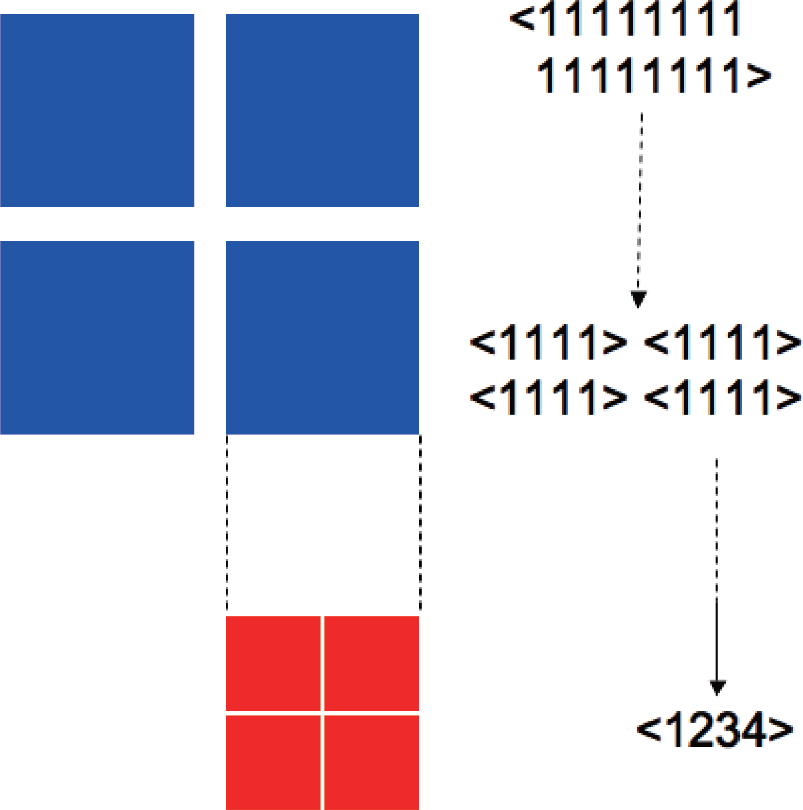
Example of 16-node system < 11 ··· 1 > that has different levels of modularity. The four 4-node subsystems < 1111 > (blue blocks) are loosely connected and easy to be decomposed, while inside each component (red blocks) is tightly connected. The degree of connection represents statistical dependency or edge information between subsystems. Such hierarchical structure can be detected by observing the decomposition path of the modular complexity Cm.
Figure 8.
Example of 16-node system < 11 ··· 1 > that has different levels of modularity. The four 4-node subsystems < 1111 > (blue blocks) are loosely connected and easy to be decomposed, while inside each component (red blocks) is tightly connected. The degree of connection represents statistical dependency or edge information between subsystems. Such hierarchical structure can be detected by observing the decomposition path of the modular complexity Cm.

Figure 9.
Contour plot of the complexity landscape of I, Cc, Cm,, and on α-β plane. (a): Contour plot superposition of Cc and Cm.(b): Contour plot superposition of
and
.(c): Contour plot of I. The color of contour plots corresponds to the color gradient of 3D plots in Figure 10;(d): Schematic representation of the system in different regions of α-β plane. Edge width represents the degree of edge information, and independence is depicted with dotted line.

Figure 10.
Landscape of complexities I, Cc, Cm,, and on α-β plane. (a): Multi-information I; (b): Cuboid-bias complexity Cc. (c): Modular complexity Cm; (d): Regularized cuboid-bias complexity
;(e): Regularized modular complexity
. All complexity measures show the complementarity intersecting with each other, satisfying the boundary conditions vanishing at α = 0 and β = 0 except the multi-information I. Note that regularized complexities
and
show singularity of convergence at α → 0 due to the regularization of infinitesimal value.


| Generalized Mean of KL-Divergence | |||
|---|---|---|---|
| Mixture Coordinates | Arithmetic Mean | Geometric Mean | |
| k-cut ζ | TSE complexity, I | ||
| < ··· >-cut ξ | CC, , Cm, | ||
© 2014 by the authors; licensee MDPI, Basel, Switzerland This article is an open access article distributed under the terms and conditions of the Creative Commons Attribution license (http://creativecommons.org/licenses/by/3.0/).
Share and Cite
MDPI and ACS Style
Funabashi, M. Network Decomposition and Complexity Measures: An Information Geometrical Approach. Entropy 2014, 16, 4132-4167. https://doi.org/10.3390/e16074132
AMA Style
Funabashi M. Network Decomposition and Complexity Measures: An Information Geometrical Approach. Entropy. 2014; 16(7):4132-4167. https://doi.org/10.3390/e16074132
Chicago/Turabian StyleFunabashi, Masatoshi. 2014. "Network Decomposition and Complexity Measures: An Information Geometrical Approach" Entropy 16, no. 7: 4132-4167. https://doi.org/10.3390/e16074132