1. Introduction
A Bayesian approach to the optimal design of experiments uses some measure of preposterior utility, or information, to assess the efficacy of an experimental design or, more generally, the choice of sampling distribution. Various versions of this approach have been developed by Blackwell [
1], and Torgerson [
2] gives a clear account. Renyi [
3], Lindley [
4] and Goel and DeGroot [
5] use information-theoretic approaches to measure the value of an experiment; see also the review paper by Ginebra [
6]. Chaloner and Verdinelli [
7] give a broad discussion of the Bayesian design of experiments, and Wynn and Sebastiani [
8] also discuss the Bayes information-theoretic approach. There is wider interest in these issues in cognitive science and epistemology; see Chater and Oaksford [
9].
When new data arrives, one can expect to improve the information about an unknown parameter θ. The key theorem, which is Theorem 2 here, gives conditions on informational functionals for this to be the case, and then, they will be called learning functionals. This class includes many special types of information, such as Shannon information, as special cases.
Section 2 gives the main theorems on learning functionals. We give our own simple proofs for completion, and the material can be considered as a compressed summary of what can be found in quite a scattered literature. We study two types of learning function, those of which we shall call the Shannon type and, in Section 3, those based on distances. For the latter, we shall make a new connection to the metric embedding theory contained in the work of Schoenberg with a link to Bernstein functions [
10,
11]. This yields a wide class of new learning functions. Following two, somewhat provocative, counter-examples and a short discussion of surprise in Section 4, we relate learning functions of the Shannon type to the theory of majorization in Section 5. Section 6 specializes learning functions on covariance matrices.
We shall use the classical Bayes formulation with θ as an unknown parameter with a prior density π(θ) on a parameter space Θ and a sampling density f(x|θ) on an appropriate sample space. We denote by fX,θ (x,θ) = f(x|θ)π(θ) the joint density of X and θand use fX(x) for the marginal density of X. The nature of expectations will be clear from the notation. To make the development straightforward, we shall look at the case of distributions with densities (with respect to Lebesgue measure) or, occasionally, discrete distributions with finite support. All necessary conditions for conditional densities, integration and differentiation will be implicitly assumed.
In Section 7, approximate Bayesian computation (ABC) is applied to problems in optimal experimental design (hence, ABCD). We believe that an understanding of modern optimal experimental design and its computational aspects needs to be grounded in some understanding of learning. At the same time, there is added value in taking a wide interpretation of optimal design as a choice, with constraints, of the sampling distribution f(x|θ). Thus, one may index f(x|θ) by a control variable z and write f(x|θ, z) or f(x(z)| θ). Certain aspects of the distribution may depend on z, others not. An experimental design can be taken as the choice of a set of z, at each of which we take one or more observations, giving a multivariate distribution. In areas, such as search theory and optimization, z may be a site at which one measures or observes with error. In spatial sampling, one may also use the term “site” for z. However, z could be a simple flag, which indicates one or another of somewhat unrelated experiments to estimate a common θ. In medicine, for example, one discusses different types of “intervention” for the same patient.
2. Information-Based Learning
The classical formulation proceeds as follows. Let U be a random variable with density fU(u). Let g(·) be a function on R+ → R and define a measure of information of the Shannon type for U with respect to g as
When
g(
u) = log(
u), we have Shannon information. When
(
γ > −1), we have a version similar to Renyi information, which is sometimes called Tsallis information [
12].
If X represents the future observation, we can measure the preposterior information of the experiment (query, etc.), which generates a realization of X, by the prior expectation of the posterior information, which we define as:
In the second term, the inner expectation is with respect to the posterior (conditional) distribution of θ given X, namely π(θ|X), and the outside expectation is with respect to the marginal distribution of X. In the last term, the expectation is with respect to the full joint distribution of X and θ. We wish to compare Ig(θ;X) with the prior information:
Theorem 1
For fixed g(u) and the standard Bayesian set-up, the pre-posterior quantity Ig(θ, X) and prior value, Ig(θ), satisfy:
for all joint distributions fX,θ (x, θ) if and only if h(u) = ug(u) is convex on R+.
We shall postpone the proof of Theorem 1 until after a more general result for functionals on densities:
Theorem 2
For the standard Bayesian set-up and a functional φ (·),
for all joint distributions fX,θ (x, θ) if and only if φ is convex as a functional:
for 0 ≤ α ≤ 1 and all π1, π2.
Proof
Note that taking expectations with respect to the marginal distribution of X amounts to a convex mixing, not dependent on θ. Thus, using Jensen’s inequality:
The necessity comes from a special construction. We show that given a functional φ(·) and a triple {π1, π2, α}, such that:
we can find a pair {f(x, θ), π(θ)}, such that
Thus, let X be a Bernoulli random variable with marginal distribution (prob{X = 0}, prob{X = 1}) = (1 − α, α). Then, it is straightforward to choose a joint distribution of θand X, such that:
from which we obtain (
1).
Proof
(of Theorem 1). We now show that Theorem 1 is a special case of Theorem 2.
Write πα(θ) = (1 − α)π1(θ) + απ2(θ). If h(u) = ug(u) is convex as a function of its argument u:
proving one direction.
The reverse is to show that if Ig is convex for all π, then h is convex. For this, again, we need a special construction. We carry this out on one dimension, the extension to more than one dimension being straightforward. For ease of exposition, we also make the necessary differentiability conditions. The second directional derivative of Ig(θ) in the space of distributions (which is convex) at π1 towards π2 is:
Let π1 represent a uniform distribution on [0,
], for some z ≥ 0, and let π2 be a distribution with support contained in [0,
]. Then, the above becomes:
Now, assume that h(z) = zg(z) is not convex at z; then h″(z) = g″ (z)z + 2g′ (z) < 0 and any choice of π2, which makes the integral on the right-hand side positive, shows that Ig(θ) is not convex at z. This completes the proof.
Theorem 2 has a considerable history of discovery and rediscovery and, in its full version, should probably be attributed to DeGroot [
13]; see Ginebra [
6]. The early results concentrated on functionals of the Shannon type, basically yielding Theorem 1. Note that the condition
h(
u) =
ug(
u) being convex on
R+ is equivalent to
being convex, which is referred to as
g(
u) being “reciprocally convex” by Goldman and Shaked [
14]; see also Fallis and Lyddell [
15].
4. Counterexamples
We show first that it is not true that information always increases. That is, it is not true that the posterior information is always more than the prior information:
A simple discrete example runs as follows. I have lost my keys. With high prior probability, p, I think they are on my desk. Suppose I have a uniform prior over all k likely other locations. However, suppose when I look on the desk that my keys are not there. My posterior distribution is now uniform on the other locations. Under certain conditions on p and k, Shannon information has gone down. For fixed p, the condition is k > k* where:
by expanding pk* in a Taylor expansion. When
, k* = 4 and pk* → e, 1 when p → 0, 1. This example is captured by the somewhat self-doubting phrase “if my keys are not on my desk, I don’t know where they are”. Note, however, that something has improved: the support size is reduced from k + 1 to k.
There is a simple way of obtaining a large class of examples, namely to arrange that there are x-values for which the posterior distribution is approximately uniform. Then, because the uniform distribution typically has low information, for such x, we can have a decrease in information. Thus, we construct examples in which f(x|θ)π(θ) happens to be approximately constant for some x. This motivates the following example.
Let Θ
× ![Entropy 16 04353f5]()
= [0
, 1]
2 with joint distribution having support on [0
, 1]
2. Let
π(
θ) be the prior distribution and define a sampling distribution:
Note that we include the prior distribution into the sampling distribution as a constructive device, not as some strange new general principle. We have in mind, in giving this construction, that when x → 1, the first term should approach zero and the second term, after multiplying by π(θ), should approach unity. Solving for a(θ) by setting
, we have
so that:
The joint distribution is then:
The marginal distribution of
X is
fX(
x) = 1 on [0
, 1], since the integral of (
9) is unity, so that (
9) is also the posterior distribution
π(
θ|x). Note that, in order for (
9) to be a proper density, we require that
for 0 ≤
θ ≤ 1.
The Shannon information of the prior is:
and of the posterior is
When
, the integrands of I1 and I0 are equal and I0 = I1. When x = 1, the integrand of I1 is zero, as expected. Thus, for a non-uniform prior, we have less posterior information in a neighborhood of x = 1, as we aimed to achieve.
Specializing
0 [0, 1] gives:
Information
I1 decreases from a maximum of
at
x = 0, through the value
I0 at
, to the value zero at
x = 1; see also
Figure 1. Thus,
I0 > I1 for
. Since the marginal distribution of
X is uniform on [0
, 1], we have the challenging fact that:
Namely, with prior probability equal to one half, there is less Shannon information in the posterior than the prior. The Renyi entropy exhibits the same phenomenon, but we omit the calculations. We might say that f(x|θ) is not a good choice sampling distribution to learn about θ.
4.1. Surprise and Ignorance
The conflict between prior beliefs and empirical data, demonstrated by these examples, lies at the heart of debates about inference and learning, that is to say epistemology. This has given rise to formal theories of surprise, which seek to take account of the conflict. Some Bayesian theories are closely related to the learning theory discussed here and measure surprise quantities, such as the difference:
Since, under the conditions of Theorem 1,
S is expected to be negative, a positive value is taken to measure surprise; see Itti and Baldi [
19].
Taking a subjective view of these issues, we may stray into cognitive science, where there is evidence that the human brain may react in a more focused way than normal when there is surprise. This is related to wider computational models of learning: given the finite computational capacity of the brain, we need to use our sensing resources carefully in situations of risk or utility. One such body of work emanates from the so-called “cocktail party effect”: if the subject matter is of sufficient interest, such as the mention of one’s own name across a crowded room, then one’s attention is directed towards the conversation. Discussions about how the attention is first captured are closely related to surprise; see Haykin and Chen [
20].
5. The Role of Majorization
We concentrate here on Shannon-type learning functions. The analysis of the last section leads to the notion that for two distributions π1(θ) and π2(θ), the second is more peaked than the first if and only if:
The statement (
10) defines a partial ordering between
π1 and
π2.
For Bayesian learning, we may hope that the ordering holds when π1 is the prior distribution and π2 is the posterior distribution. We have seen from the counterexamples that it does not hold in general, but, loosely speaking, always holds in expectation, by Theorem 1. However, it is natural to try to understand the partial ordering, and we shall now indicate that the ordering is equivalent to a well-known majorization ordering for distributions.
Consider two discrete distributions with n-vectors of probabilities\
and
, where
. First, order the probabilities:
Then, π2 is said to majorize π1, written π1 ≼ π2, when:
for
j = 1
, . . . , n (equality for
j =
n). The standard reference is Marshall and Olkin [
22], where one can find several equivalent conditions. Two of the best known are:
A1. there is a doubly stochastic matrix Pn×n, such that π1 = Pπ2;
A2.
for all continuous convex functions h(x).
Condition A2 shows that, in the discrete case, the partial ordering (
10) is equivalent to the majorization of the raw probabilities.
We now extend this to the continuous case. This generalization, which we shall also call ≼, to save notation, has a long history, and the area is historically referred to as the theory of the “rearrangements of functions” to respect the terminology of Hardy
et al. [
23]. It is particularly well-suited to probability density functions, because
∫ π1(
θ)
dθ =
∫π2(
θ)
dθ = 1. The natural analogue of the ordered values in the discrete case is that every density
π has a unique density
π̃ , called a “decreasing rearrangement”, obtained by a reordering of the probability mass to be non-increasing, by direct analogy with the discrete case above. In the theory,
π and
π̃ are then referred to as being equimeasurable, in the sense that the supports are transformed in a measure-preserving way.
There are short sections on the topic in Marshall and Olkin [
22] and in Müller and Stoyan [
24]. A key paper in the development is Ryff [
25]. The next paragraph is a brief summary.
Definition 2
Let π(z) be a probability density and define m(y) = μ{z : π(z) ≥ y}. Then:
is called the decreasing rearrangement of π(z).
The picture is that the probability mass (in infinitely small intervals) is moved, so that a given mass is to the left of any smaller mass. For example, for the triangular distribution:
we have:
Definition 3
We say that π2 majorizes π1, written π1 ≼ π2, if and only if, for the decreasing rearrangements,
for all c > 0.
Define a doubly stochastic kernel P(x, y) ≥ 0 on (0,∞), that is:
There is a list of key equivalent conditions to ≼, which are the continuous counterparts of the discrete majorization conditions. The first two generalize A1 and A2 above.
B1. π1(θ) = ∫Θ P(θ, z)π2(z)dz for some non-negative doubly stochastic kernel P(x, y).
B2. ∫Θ h(π1(z))dz ≤ ∫Θ h(π2(z))dz for all continuous convex functions h.
B3. ∫Θ (π1(z) − c)+dz ≤ ∫Θ (π2(z) − c)+dz for all c > 0.
Condition B2 is the key, for it shows that in the univariate case, if we assume that
h(
u) =
ug(
u) is continuous and convex, (
10) is equivalent to
π1(
θ) ≼
π2(
θ). We also see that ≼ is equivalent to standard first order stochastic dominance of the decreasing rearrangements, since
is the cdf corresponding to
π̃(
θ). Condition B3 says that the probability mass under the density above a “slice” at height
c is more for
π2 than for
π1.
We can summarize this discussion by the following.
Proposition 1
A functional is a learning functional of the Shannon type (under mild conditions) if and only if it is an order-preserving functional with respect to the majorization ordering on distributions.
The role of majorization has been noticed by DeGroot and Fienberg [
26] in the related area of proper scoring rules.
The classic theory of rearrangements is for univariate distributions, whereas, as stated, we are interested in θ of arbitrary dimension. In the present paper, we will simply make the claim that the interpretation of our partial ordering in terms of decreasing rearrangements can indeed be extended to the multivariate case. Heuristically, this is done as follows. For a multivariate distribution, we may create a univariate rearrangement by considering a decreasing threshold and “squashing” all of the multivariate mass for which the density is above the threshold to a univariate mass adjacent to the origin. Since we are transforming multivariate volume to area, care is needed with Jacobians. We can then use the univariate development above. It is an instructive exercise to consider the univariate decreasing rearrangement of the multivariate normal distribution, but we omit the computations here.
6. Learning Based on Covariance Functions
If we restrict our functionals to those which are only functionals of covariance matrices, then we can prove wider results than just for the trace. Dawid and Sebastiani [
27] (Section 4) refer to dispersion-coherent uncertainty functions and, where their results are close to ours, we differ only by assumptions.
We use the notation A ≥ 0 to mean that a symmetric matrix is non-negative definite.
Definition 4
For two n × n symmetric non-negative definite matrices A and B, the Loewner ordering A ≥ B holds when A − B ≥ 0.
Definition 5
A function φ : A ↦ R on the class of non-negative definite matrices A is said to be Loewner increasing (also called matrix monotone) if A ≥ B ⇒ φ(A) ≥ φ(B).
Theorem 7
A function φ is Loewner increasing and concave on the class of covariance matrices Γ (π) if and only if −φ is a learning function on the corresponding distributions.
Proof
Assume φ is Loewner increasing. To simplifying the notation, we call μ(π) and Γ(π) the mean vector and covariance matrix, respectively, of the random variable Z with distribution π. Now, consider a mixed density πα = (1 − α)π1 + απ2. Then, with obvious notation,
for 0 ≤ α ≤ 1, since (μ1 − μ2)( μ1 − μ2)T is non-negative definite. Then, since φ is Loewner increasing and concave, φ(Γ(πα)) ≥ φ ((1 − α)Γ(π1) + αΓ(π2)) ≥ (1 − α)φ(Γ(π1)) + αφ(Γ(π2)), and by Theorem 2, −φ is a learning function.
We first prove the converse for matrices Γ and Γ̃ = Γ+zzT , for some vector z. Take two distributions with equal covariance functions, but with means satisfying μ1 − μ2 = 2z. Then,
Now assume −φ is a learning function. Then, by concavity,
In general, we can write any Γ̃ ≥ Γ as
, for a sequence of vectors {z(i)}, i = 1, . . . ,m, and the result follows by induction from the last result.
Most criteria used in classical optimum design theory (in the linear regression setting) when applied to covariance matrices are Loewner increasing. If, in addition, we can claim concavity, then by Theorem 7, the negative of any such function is a learning function. We have seen in Section 3 that –trace(Γ) is a learning function, while −log det(Γ) corresponding to D-optimality is another example.
For the normal distribution, we can show that for two normal density functions, π1 and π2, with covariance Γ1 and Γ2, respectively, we have that for any Shannon-type learning function Ig(θ1) ≤ Ig(θ2) if and only if det(Γ1) ≥ det(Γ2). We should note that in many Bayesian set-ups, such as regression and Gaussian process prediction, we have a joint multivariate distribution between x and θ. Suppose that, with obvious notation, the joint covariance matrix is:
Then, the posterior distribution for θ has covariance
. Thus, for any Loewner increasing φ, it holds that −φ(π(θ)) ≤ −EX(φ(π(θ|X))), by Theorem 7. However, as the conditional covariance matrix does not depend on X, we have learning in the strong sense; −φ(π(θ)) ≤ −φ(π(θ|X)). Classifying learning functions for θ and Γθ,X in the case where they are both unknown is not yet fully developed.
7. Approximate Bayesian Computation Designs
We now present a general method for performing optimum experimental design calculations, which, combined with the theory of learning outlined above, may provide a comprehensive approach. Recall that in our general setting, a decision about experimentation or observation is essentially a choice of the sampling distribution. In the statistical theory of the design of experiments, this choice typically means a choice of observation sites indexed by a control or independent variable z.
Indeed, we will have examples below in this category. However, the general formulation is that we want to maximize ψ over some restricted set of sampling distributions f(x|θ) ∈ . A choice of f we call generalized design. Below, we will have one non-standard example based on selective sampling. Note that we shall always assume that the prior distribution π(θ) is fixed, which is independent of the choice of f. Then, recalling our general information functional as φ(π), the design optimization problem is (for fixed π):
where we stress the dependence of the random variable X on the design and, thereby, on the sampling distribution f, by adding the subscript D.
If the set of sampling distributions f is specified by the control variable z, that is the choice of the sampling distribution f(x|θ, z) amounts to selecting z ∈ Z, then the maximization problem is:
In the examples that we consider below, the sampling distribution will be indexed by a control variable z.
An important distinction should be made between what we shall here call linear and non-linear criteria. By a more general utility problem being linear, we mean that there is a utility function U(θ, x), such that, when we seek to minimize, again over choice f,
where the last expectation is with respect to the joint distribution of XD and θ. In terms of integration, this only requires a single double integral. The non-linear case requires the evaluation of an “internal” integral for Eθ|XDU(XD, θ) and an external integral for EXD. It is important to note that Shannon-type functionals are special types of linear functionals where U(θ,XD) = g(π(θ|XD)). The distance-based functionals are non-linear in that they require a repeated single integral.
This distinction is important when other costs or utilities are included in addition to those coming from learning. Most obvious is a cost for the experiment. This could be fixed, so that no preposterior analysis is required, or it might be random in that it depends on the actual observation. For example one might add an additional utility U(XD) solely dependent of the outcome of the experiment: if it really does snow, then snow plows may need to be deployed. The overall (preposterior) expected value of the experiment might be:
In this way, one can study the exploration-exploitation problem, often referred to in search and optimization.
We now give a procedure to compute
ψ for a particular choice of sampling distribution
f ∈
. We assume that
f(
x|θ) and
π(
θ) are known. If the functional
φ is non-linear, we have to obtain the posterior distribution
π(
θ|XD) before evaluating
φ. For simplicity, we use ABC rejection sampling (see Marjoram
et al. [
28]) to obtain an approximate sample from
π(
θ|XD) that allows us to estimate the functional
φ(
π(
θ|XD)). In many cases, it is hard to find an analytical solution for
π(
θ|XD), especially if
f(
x|θ) is intractable. These are the cases where ABC methods are most useful. Furthermore, ABC rejection sampling has the advantage that it is easily possible to re-compute
φ̂(
π(
θ|XD)) for different values of
XD, which is an important feature, because we have to integrate over the marginal distribution of
XD in order to obtain
ψ(
f) = E
XDφ(
π(
θ|XD)).
For a given f ∈ , we find the estimate ψ̂ by integrating over φ̂(π(θ|XD)) with respect to the marginal distribution fX. We can achieve this using Monte Carlo integration:
for
. The ABC procedure to obtain the estimate φ̂(π(θ|xD)) given xD is as follows.
- (1)
Sample from π(θ) : {θ1, . . . , θH}.
- (2)
For each θi, sample from f(x|θi) to obtain a sample:
. This gives a sample from the joint distribution: fX,θ.
- (3)
For each θi, compute a vector of summary statistics: T(x(i)) = (T1(x(i)), . . . , Tm(x(i))).
- (4)
Split
T-space into disjoint neighborhoods
![Entropy 16 04353f6]()
.
- (5)
Find the neighborhood
![Entropy 16 04353f6]()
for which
T(
xD) ∈
![Entropy 16 04353f6]()
and collect the
θi for which
T(
x(i)) ∈
![Entropy 16 04353f6]()
, forming an approximate posterior distribution
π̃(
θ|T), which if
T is approximately sufficient, should be close to
π(
θ|xD). If
T is sufficient, we have that
π̃(
θ|T) →
π(
θ|xD) as
| ![Entropy 16 04353f6]() |
| → 0.
- (6)
Approximate π(θ|xD) by π̃(θ|T).
- (7)
Evaluate φ(π(θ|xD)) by integration (internal integration).
Steps 1–4 need to be conducted only once at the outset for each f ∈ ; only Steps 5–7 have to be repeated for each xD ~ fX.
For the linear functional, explained above, we do not even need to compute the posterior distribution, π(θ|xD), if we are happy to use the naive approximation to the double integral:
where
are independent draws from the joint distribution f(x, θ) = f(x|θ)π(θ).
The optimum ψ(f) for f ∈ may be found by employing any suitable optimization method. In this paper, we intend to focus on the computation of ψ̂(f). Therefore, in the illustrative examples below, we take a “crude” optimization approach, that is we estimate ψ(f) for a fixed set of possible choices for f and compare the estimates.
The basic technique of ABCD was introduced in Hainy
et al. [
29], but here, we present it fully embedded into statistical learning theory. Note that related different procedures utilizing MCMC chains were independently developed in Drovandi and Pettitt [
30] and Hainy
et al. [
31].
We now present two examples that are meant to illustrate the applicability of ABCD to very general design problems using non-linear design criteria. Although these examples are rather simple and may also be solved by analytical or numerical methods, their generalizations become intractable using traditional methods.
7.1. Selective Sampling
When the background sampling distribution is f(x|θ), we may impose prior constraints of which data we accept to use. Such models in greater generality may occur when observation is cheap, but the use of observation is expensive, for example computationally. We can call this “selective sampling”, and we present a simple example.
Suppose in a one-dimensional problem that we are only allowed to accept observations from two slits of equal width at z1 and z2. Here, the model is equivalent (in the limit as the slit widths become small) to replacing f(x|θ) by the discrete distribution:
If we have a prior distribution π(θ) and f(x|z1, z2) = ∫ f(x|θ, z1, z2)π(θ)dθ denotes the marginal distribution of x, the posterior distribution is given by:
To simplify even further, we take as a criterion:
The maximum is a limiting version of Tsallis entropy and is a learning functional.
Now consider a special case:
The preposterior:
can be calculated explicitly. If z2 ≥ z1 and zi ∈ [−a, a], then:
Next, we show how this example can be solved using ABCD. Due to the special structure of the sampling distribution in this example, we modified our ABC sampling strategy slightly.
- (1)
For fixed z1 and z2, sample H numbers {θ(j), j = 1, . . . ,H} from the prior.
- (2)
For each θ(j), repeat:
- (a)
sample z(k) ~ π(z|θ(j)) until #{z(k) ∈ {Nε (z1),Nε (z2)}}= Kz, where Nε(z) = [z − ε/2, z + ε/2];
- (b)
drop all z(k) ∉ {Nε(z1),Nε(z2)};
- (c)
sample x(j) from discrete distribution with probabilities
, i = 1, 2.
- (3)
For i = 1, 2, select all θ(j) for which x(j) = i, compute kernel density estimate for these θ(j) and obtain maximum → φ̂(π̂(θ|x = i, z1, z2)).
- (4)
.
We performed our ABC sampling strategy for this example for a range of parameters for the slit neighborhood length ε (ε = 0.005, 0.01, 0.05), H (H = 100, 1,000, 10,000) and Kz (Kz = 50, 100, 200) in order to assess the effect of these parameters on the accuracy of the ABC estimates of the criterion ψ. The most notable effect was found for the ABC sample size H.
Figure 2 shows the estimated values of the criterion,
ψ̂, for the special case where
z2 = −
z1 when
a = 1
.5. We set
ε = 0
.01,
Kz = 100. The ABC sample size
H is set to
H = 100 (left),
H = 1
, 000 (center), and
H = 10
, 000 (right). The criterion was evaluated at the eight points (
z1 = 0
.1
, 0
.3
, 0
.5
, 0
.7
, 0
.9
, 1
.1
, 1
.3
, 1
.5). The theoretical criterion function
ψ(
z1) is plotted as a solid line.
7.2. Spatial Sampling for Prediction
This example is also a simple version of an important paradigm, namely optimal sampling of a spatial stochastic process for good prediction. Here, the stochastic process labeled X is indexed by a space variable z, and we write Xi = Xi(zi), i = 1, . . . , n to indicate sampling at sites (the design) Dn = {z1, . . . , zn}. We would typically take the design space, Z, to be a compact region.
We wish to compute the predictive distribution at a new site zn+1, namely xn+1(zn+1), given xD = x(Dn) = (x1(z1), . . . , xn(zn)). In the Gaussian case, the background parameter θ could be related to a fixed effect (drift) or the covariance function of the process, or both. In the analysis, xn+1 is regarded as an additional parameter, and we need its (marginal) conditional distribution.
The criterion of interest is the maximum variance of the (posterior) predictive distribution over the design space:
This functional is learnable, since it is is a maximum of a set of variances, each one of which is learnable.
Referring back to how the general design optimization problem that was stated in (
11), the posterior predictive distribution of
xn+1 may be interpreted as the posterior distribution in (
11). The optimality criterion
ψ is found by integrating
φ with respect to
X1, . . . ,Xn.
The strategy is to select a design Dn and then perform ABC at each test point zn+1. The learning functional φ(xD) is estimated by generating the sample
at the sites {z1, z2, . . . , zn, zn+1} and calculating:
where
, we have
if
, and
.
In order to estimate ψ(Dn) = EXD(φ(XD)), we obtain a sample
from the marginal distribution of the random field at the design Dn and perform Monte Carlo integration:
For each
from the marginal sample, we use the sample I to compute
in order to save computing time. We then vary the design using some optimization algorithm.
A simple example is adopted from Müller
et al. [
32]. The observations (
x1(
z1)
, x2(
z2)
, x3(
z3)
, x4(
z4)) are assumed to be distributed according to a one-dimensional Gaussian random field with mean zero, a marginal variance of one and
zi ∈ [0
, 1]. We want to select an optimal design
D3 = (
z1, z2, z3), such that:
is minimal.
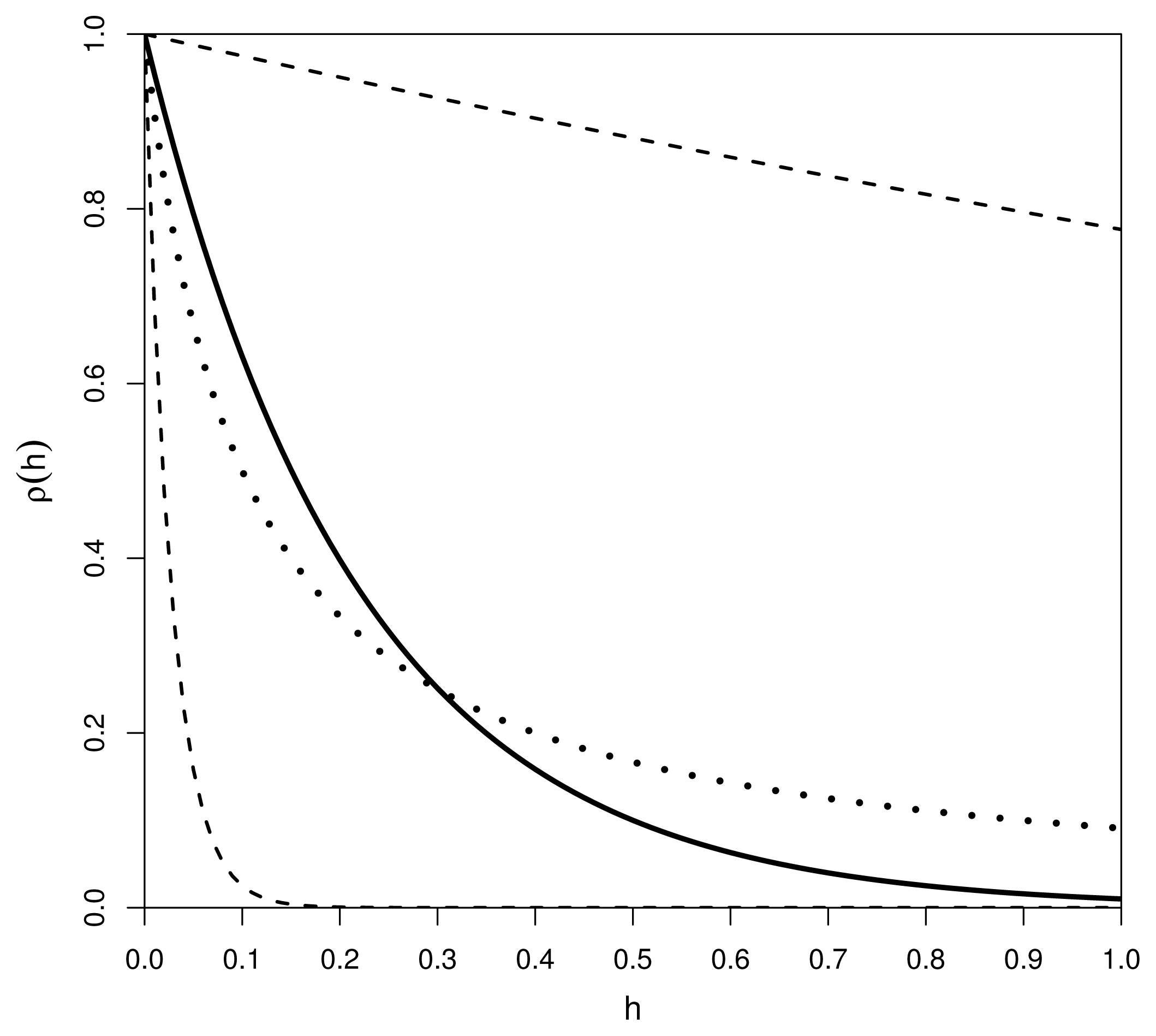
We assume the Ornstein–Uhlenbeck process with correlation function
ρ(
|s −
t|;
θ) =
e−θ|s−t|. Two prior distributions for the parameter
θ are considered. The first one is a point prior at
θ = log(100), so that
ρ(
h) =
ρ (
h; log(100)) = 0
.01
h. This is the correlation function used by Müller
et al. [
32] in their study of empirical kriging optimal designs. The second prior distribution is an exponential prior for
θ with scale parameter
λ = 10 (
i.e.,
θ ~ Exp(10)). The scale parameter
λ was chosen, such that the average correlation functions of the point and exponential priors are similar. By that, we mean that the average of the mean correlation function for the exponential prior over all pairs of sites
s and
t, E
s,t[E
θ{
ρ(
|s−
t|;
θ)
|θ ~ Exp(
λ)}] = E
s,t[1
/(1+
λ|s−
t|)], matches the average of the fixed correlation function
ρ(
|s −
t|; log(100)) = 0
.01
|s−t| over all pairs of sites
s and
t, E
s,t[0
.01
|s−t|]. The sites are assumed to be uniformly distributed over the coordinate space.
To be more specific, first, for each site
s ∈
![Entropy 16 04353f5]()
, the average correlation to all other sites
t ∈
![Entropy 16 04353f5]()
is computed. Then, these average correlations are averaged over all sites
s ∈
![Entropy 16 04353f5]()
. For the point prior, the average correlation is
, and for the exponential prior, the value is
. If
λ = 10, we have E
s,t[E
θ{
ρ(
|s −
t|;
θ)
|θ ~ Exp(10)}] = 0
.3275.
Figure 3 depicts the distributions of the correlation function
ρ(
h;
θ) = exp(−
θh) under the two prior distributions. The solid line corresponds to the fixed correlation function
ρ(
h;
θ = log(100)) = 0
.01
h. The dotted line and the two dashed lines represent the mean correlation function and the 0.025- and 0.975-quantile functions for
ρ(
h;
θ) under the prior
θ ~ Exp(10).
We estimated the criterion on a grid with spacing 0.05 for the design points
z1 and
z3 (
z2 is fixed at
z2 = 0
.5). We set
G = 1
, 000,
H = 5 · 10
6 and
ε = 0
.01 for each design point. The sample
is simulated at all points
z of the grid prior to the actual ABC algorithm. In order to accelerate the computations, it is then reused for all possible designs
D3 to estimate each
,
i = 1
, . . . ,G, in (
12). The sample size
H = 5 · 10
6 was deemed to provide a sufficiently exhaustive sample from the four-dimensional normal vector (
x1(
z1)
, x2(
z2)
, x3(
z3)
, x4(
z4)) for any
zi ∈
Z, so that the distortive effect of using the same sample for the computations of all
is only of negligible concern for our purposes of ranking the designs.
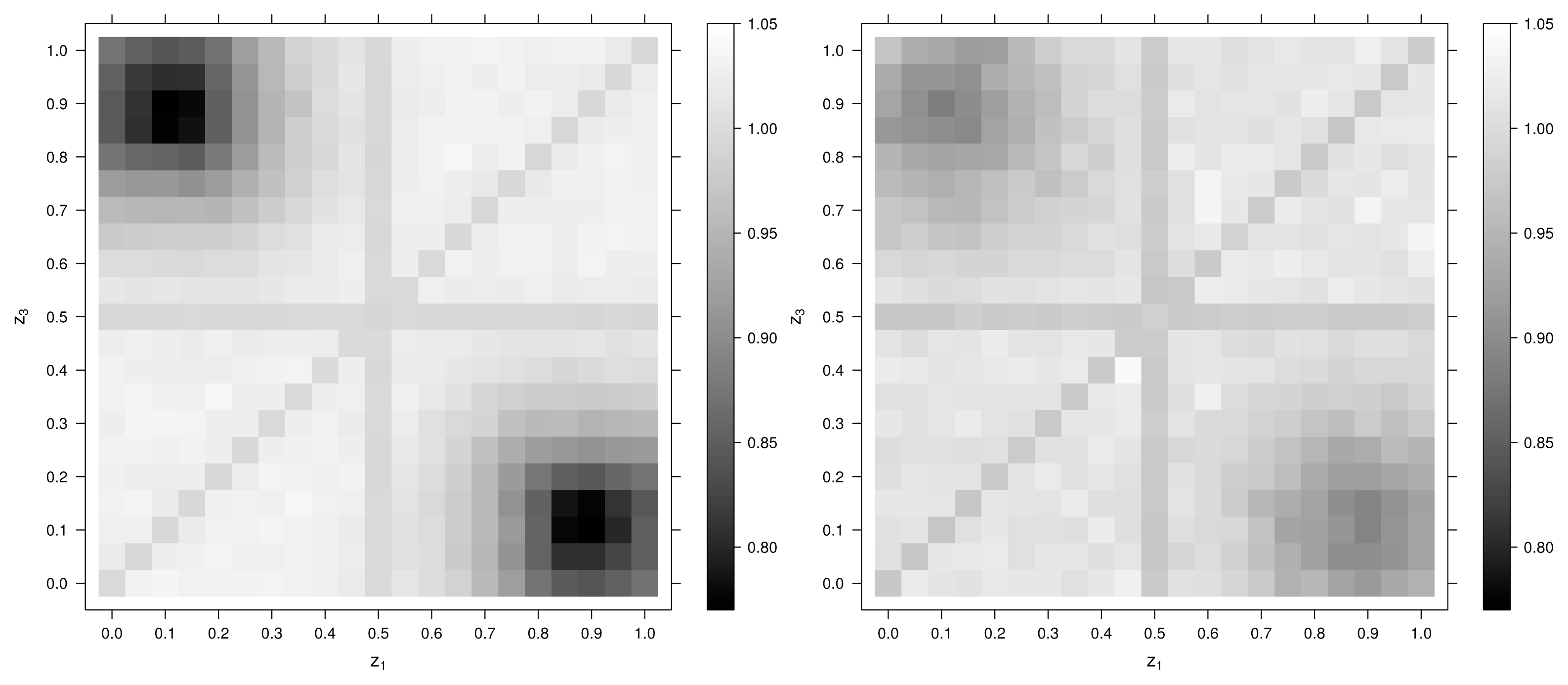
Figure 4 (left) shows the map of estimated criterion values, −
ψ̂ (
D3), when the prior distribution of
θ is the point prior at
θ = log(100). It can be seen that the minimum of the criterion is attained at about (
z1, z3) = (0
.9
, 0
.1) or (
z1, z3) = (0
.1
, 0
.9), which is comparable to the the results obtained in Müller
et al. [
32] for empirical kriging optimal designs. Note that the diverging criterion values at the diagonal and at
z1 = 0
.5 and
z3 = 0
.5 are attributable to a specific feature of the ABC method used. At these designs, the actual dimension of the design is lower than three, so for a given
ε, there are more elements in the neighborhood than for the other designs with three distinctive design points. Hence, a much larger fraction of the total sample,
, is included in the ABC sample,
. Therefore, the values of the criterion get closer to the marginal variance of one. In order to avoid this effect, the parameter ε would have to be adapted in these cases. Alternatively, one could use other variants of ABC rejection, where the fixed number of N elements of
with the smallest distance to the draw
are constituting the ABC posterior sample, making it necessary to compute and sort out the distances for each
.
Figure 4 (right) gives the estimated criterion values, −
ψ̂(
D3), when the prior of
θ is
θ ~ Exp(10). Due to the uncertainty of the prior parameter
θ, the optimal design points for
z1 and
z3 slightly move to the edges, which is also in accordance with the findings of Müller
et al. [
32].

 = [0, 1]2 with joint distribution having support on [0, 1]2. Let π(θ) be the prior distribution and define a sampling distribution:


