Article

Spatiotemporal Scaling Effect on Rainfall Network Design Using Entropy

1
The Experimental Forest, College of Bio-Resources and Agriculture, National Taiwan University, No.12 Chien-Shan Rd. Sec.1 Jushan Township, Nantou 55750, Taiwan
2
Department of Natural Resources, Chinese Culture University, Taipei 11114, Taiwan
3
Department of Civil Engineering, National Taipei University of Technology, Taipei 10608, Taiwan
*
Author to whom correspondence should be addressed.
Entropy 2014, 16(8), 4626-4647; https://doi.org/10.3390/e16084626
Submission received: 28 January 2014 / Revised: 26 May 2014 / Accepted: 7 August 2014 / Published: 18 August 2014
(This article belongs to the Special Issue Entropy in Hydrology)

Abstract

:
Because of high variation in mountainous areas, rainfall data at different spatiotemporal scales may yield potential uncertainty for network design. However, few studies focus on the scaling effect on both the spatial and the temporal scale. By calculating the maximum joint entropy of hourly typhoon events, monthly, six dry and wet months and annual rainfall between 1992 and 2012 for 1-, 3-, and 5-km grids, the relocated candidate rain gauges in the National Taiwan University Experimental Forest of Central Taiwan are prioritized. The results show: (1) the network exhibits different locations for first prioritized candidate rain gauges for different spatiotemporal scales; (2) the effect of spatial scales is insignificant compared to temporal scales; and (3) a smaller number and a lower percentage of required stations (PRS) reach stable joint entropy for a long duration at finer spatial scale. Prioritized candidate rain gauges provide key reference points for adjusting the network to capture more accurate information and minimize redundancy.

1. Introduction

The most crucial information required for planning, constructing, and operating hydraulic structures is rainfall data. The objective of a rainfall network is to design hydraulic structures efficiently and economically, according to the researched rainfall data [1]. However, because of topography, rain patterns, and effects of time, the spatial and temporal distributions of precipitation are uneven. Consequently, planning a suitable and optimal rain gauge station network is a challenging task. Research shows that even when two rain gauge stations are in close proximity to each other (5 km), the correlation coefficient of their precipitation time sequences may be lower than 0.5 [2]. This low correlation complicates the design and modulation of a rainfall network.
A reliable rainfall network can provide the immediate and precise precipitation data that is crucial to designing and placing hydraulic structures such as flood-prevention drainages. However, the number of rain gauge stations required may differ significantly from one watershed to another. In the past, stations were usually built without any standardization, according to the population density, assigned budget of each area, or the traffic feasibility to the stations. Hence, a problem of representative rainfall distribution and possible data redundancy may result. The World Meteorological Organization (WMO) [3] prescribes the minimum density of rainfall networks under various topographical and meteorological conditions, in particular, 25 km2 per station on mountainous islands with irregular precipitation, one of which is Taiwan, the selected case in this study.
The optimization of a rainfall network has to satisfy two crucial criteria—spatial and temporal. Previous studies have mainly focused on the estimation of the location, distribution, and priority of rain gauge stations. However, determining the minimum number and optimal location of stations requires further investigation. Furthermore, the effect of spatiotemporal scaling on network design is yet to be analyzed. Applications to groundwater quality monitoring networks, stream gauge networks, and water distribution networks have increased in recent years. The methods used in network research related to entropy include least square methods and entropy [4], kriging [5], information entropy [622], and combined kriging and information entropy [2325]. In particular, the information entropy approach has been widely adopted since the 1970s for hydrologic data collection network design and uncertainty evaluation [2633].
The effects of heterogeneity and of scale and scaling continue to be significant issues in hydrologic research. Despite the progress that has been achieved in the past 20 years, considerable interest and much research remain centered on these issues [34]. Disaggregation-aggregation approaches were illustrated to link catchment-scale and point-scale state variables, which permit an empirical large-scale model that still retains some essence of small-scale physics [35]. The analysis of rainfall data from buoys on the ocean, the microwave imager (TMI) and precipitation radar (PR) on board the Tropical Rainfall Measuring Mission (TRMM) satellite shows that TMI and PR satellite data from 2.5° × 2.5° areas centered on the buoys consistently agree well with the buoys on both annual and seasonal timescales, but the monthly point measurement of buoys exhibited large differences with TRMM data [36]. Singh [37] addressed the complete entropy theory and its applications in environmental and water engineering, and most importantly, several entropy measures, including directional information transfer index, total correlation, and maximum information minimum redundancy, were introduced. Nevertheless, few studies have been conducted to evaluate the possible spatiotemporal scaling issue for network design. The proposed scheme for analyzing an optimal rainfall network involves kriging to generate the rainfall data of the candidate rain gauge stations, and entropy to evaluate the uncertainty in different combinations of spatial and temporal scales. In this study, we evaluate the spatiotemporal scaling effect on rain gauge network design and suggest optimal configuration. In particular, because records of several typhoon rainfall events, together with monthly, six dry and wet months, and annual rainfall, were analyzed, an optimal rain gauge network can be optimized by the hydrologic or climatic consideration, either short- or long-duration based. Once the optimal network design with maximum information and minimum redundancy is established, rainfall characteristics can be obtained to provide the key reference for the hydrologic planning for the watershed.

2. Methodology

This study involved the following steps: (1) determining the different combinations of spatial and temporal scales and delineating the study area; (2) applying kriging to existing rainfall data to generate the rainfall data of the candidate rain gauge stations for a certain combination; (3) determining the priority sequence of the candidate rain gauge stations and evaluating the minimum number required; and (4) summarizing the spatiotemporal scaling effect.

2.1. Spatiotemporal Scale

Stewart et al. [38] pointed out two distinct problems involved in scaling: (1) the requirement for a set of concepts that will allow the correct partitioning of the water balance at any given scale; and (2) the concepts that will allow information gathered at one scale to be used in making predictions at other scales. To solve these two problems, the possible scaling effect should be addressed first. In this study, spatial scales for 1 × 1, 3 × 3, and 5 × 5 km grids were partitioned to delineate a study area comprising 327.86 km2. A total of 346, 45, and 20 grids were created, respectively. The center of each grid was assigned the location of a candidate rain gauge station. At each of the three different spatial scales, hourly records for typhoon events, monthly, six dry and wet months and annual rainfall were individually analyzed. Hourly data are used to investigate fluctuations of short duration for extreme events while the monthly, six dry and wet months and annual data depict the possible seasonal and annual trends or variations. Therefore, a total of fifteen combinations for different conditions are evaluated.

2.2. Kriging

Kriging is a geostatistical method for interpolating random spatial variations in rainfall data to estimate linear grid points [3943]. In this study, we use the exponential model to fit the semi-variogram from the measurements of rainfall [24]:
γ ( h ) = b [ 1 - exp ( - h a ) ]
where a denotes the range parameter, and b denotes the sill; that is, the critical variance in the spatial independence is as high as 3a.
In particular, three independent short-term rainfall measurements from the 50 rain gauges were used to verify the kriging results.

2.3. Entropy

The information entropy introduced by Shannon [44,45] is based on probabilities. The entropy value is used to estimate uncertainties:
H ( x ) = - i = 1 n p i log ( p i )
where H(x) is the entropy value and pi is probability.
Shannon’s entropy [45] is a measure of information content, which depends on the current level of knowledge or uncertainty. Mathematically, the amount of information is inversely related to the probability of occurrence. The basic assumptions of the entropy are the amount of information, I(p), being a real nonnegative measure, additive, and a continuous function of probability p. For the rational numbers, the function of I(p) obeys the same formula as the log function. For any discrete probability distribution, Shannon’s entropy is expressed as:
H ( x 1 ) = - i p i ln  p i
where pi is the probability of event xi. Equation (3) refers only to the information state before receiving data. Thus, H(x1) measures the average amount of information. H(x1) = 0 when the event is certain (pi = 0 or 1) and there is no surprise. Because of the uniformity resulting in an inability to believe any outcome being more likely than any other, uniform distribution results correspond to maximum ignorance. Maximum entropy can be seen as a generalization of the classical principle of indifference and can be used to obtain unbiased probability assessments.
The rainfall information of two rain gauge stations may be overlapped. Therefore the rainfall information of the two rain gauge stations can become two variables x1 and x2. Corresponding to Equation (3), the joint entropy of two variables is [24]:
H ( x 1 , x 2 ) = - i j p i j ln  p i j
For three variables of x1, x2, and x3, the joint entropy is [24]:
H ( x 1 , x 2 , x 3 ) = - i j k p i j k ln  p i j k
where pijk is the joint probability of x1, x2, and x3.
When the x1 rain gauge station is examined to record rainfall data, the remaining uncertainty of the x2 rain gauge station will be exhibited by the conditional entropy. The probability of x2 under the influence of x1’s condition can be shown as below [24]:
p ( x 2 x 1 ) = p j i = p i j p i
Thus:
H ( x 1 , x 2 ) = H ( x 2 x 1 ) + H ( x 1 )
The joint entropy that can measure the amount of information of the joint events is derived by Equation (7) with conditional probability [24]:
H ( x 2 x 1 ) = H ( x 1 , x 2 ) - H ( x 1 )
where H(x2|x1) is the conditional entropy of x2 given x1. To find out the amount of mutual or overlapped information of the two stations, a transferable information calculation can be utilized to do so, as if using the x1 rain gauge station to forecast information from the x2 rain gauge station.

2.4. Optimization of Network Design

The significance of each rain gauge station in its network can be determined from its entropy value. The greater the value, the higher the uncertainty; thus, each station is prioritized according to the descending order of entropy values. After confirming the first station, which has the greatest entropy value, the rest are selected and added one at a time, according to the inferiority of the system and overlapped information. To minimize the system’s uncertainty, the standardization of determining the second most important station in the sequence is set as [24]:
M i n { H ( x 2 ) - H ( x 2 x 1 ) }
Then, the n-th to be added is [24]:
M i n { H ( x 1 , x 2 , , x n - 1 ) - H [ ( x 2 x 1 , x 2 , , x n - 1 ) ] }
In the calculation, therefore, the greatest H[(xn|x1,x2,···,xn−1)] can be selected to arrange the order of data overlap of all the stations, in which the station with minimum overlap is the first to be added to the network, and the station with maximum overlap is the last to be added.
The sequence of prioritized stations determined by the entropy values can also be used as the sequence of station elimination. In each selection stage, the objective is to ascertain the maximum entropy value of each selected station. Stations are subsequently added according to the gradual increase in the joint entropies. However, the joint entropy does not increase sufficiently to show any differences when it reaches a certain number and attains a definite value. In other words, adding more stations has a very limited effect on the network system. The exponential model is applied to the correlation graph of the station numbers and H[(xn|x1,x2,···,xn−1)] to detect the critical data volume and the supposed number of stations. The coefficient km denotes the specific value of the m-th entropy value, as compared with all entropy values of the study area; it is assumed to be used as the reveal data volume of the m-th station. Assuming n stations in the study area and a number of basic stations have been selected, and the addition of new candidate rain gauge stations is prioritized on the basis of the entropy value, the definition of km in this study can be expressed as [24]:
k m = H ( x 1 , x 2 , , x m ) H ( x 1 , x 2 , , x m , , x n - 1 , x n ) ,             m < n
and k1, k2,..., km,..., kn−1, kn < 1. Hence, in determining the number of stations in a catchment area, a threshold value k m * must be set, and by setting a limit such as k m > k m *, the number can be secured.
On the other hand, the threshold value is determined by the increasing efficiency revealed by the increment of km. In this study, km is set to 0.95, which is 95% of the information. Hence, if the number of rain gauge stations in the existing network is greater than that in the candidate network, those existing stations sequenced behind the candidate station are to be eliminated; otherwise, more stations are added.
In this study, there are fifteen combinations of different spatiotemporal scales. To evaluate the efficiency to the number km, we define the percentage of required stations reaching 95% information PRS (%) as:
P R S ( % ) = n ( k m ) n × 100 % , m < n
PRS is used to evaluate the efficiency of the sequence of prioritized stations. The number of prioritized stations may be the same at different combinations of spatiotemporal scales. However, lower PRS can be regarded as more efficient to reach the total 95% threshold value of measured uncertainty with fewer stations.

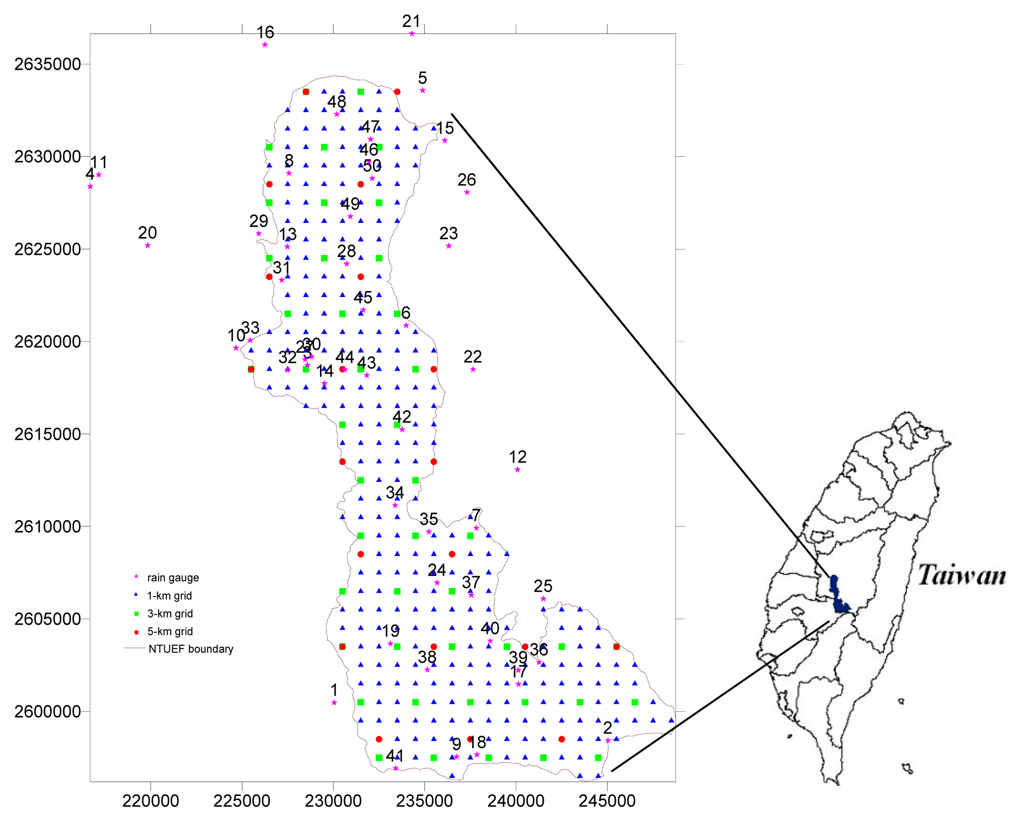
2.5. Study Area and Data

To illustrate and evaluate the proposed model, rainfall data within and near the National Taiwan University Experimental Forest (NTUEF) is used to demonstrate an optimal rainfall network. Located upstream on the Zhuoshui River, the geographical site lies between 23°48′49″ and 23°28′10″N and 121°45′16″ and 121°59′15″E, accounting for an approximate area of 327.86 km2 (Figure 1). The catchment area extends from the Mt. Jade (elevation 3952 m, the highest peak in Taiwan) to Gueitsuto (220 m). Coursing through major forestland within the Chenyulan catchment, the river flows over 41.4 km, with an average slope of 2.7%. Most of the catchment is covered by mature forests, and the geological features of this region include a complex suite of rocks, such as granite, gneiss, schist, sandstone, conglomerate, and marl. Because of differences in altitude, the climate is divided into subtropical, warm temperate, cold temperate, subfrigid, and frigid zones. The mean annual temperature ranges between a low of 4 °C (Mt. Jade) and a high of 23 °C (Jushan). The NTUEF area usually experiences enhanced rainfall, and it receives an average (1992–2012) rainfall of 2408 mm; however, the rainfall is unevenly distributed, with more than 70% of it occurring between May and September. The annual rainfall increases from north to south and east to west, and consists of several centers (Figure 2a). During the period 1992 to 2012, the most severe rainfall event, Typhoon Morakot, which occurred 5 August to 9 August 2009, poured almost the entire average annual rainfall within a few days (Figure 2b). The largest rainfall recorded by the Alishan weather station (bottom left near the boundary in Figure 1) is 2884 mm, which caused a large-scale landslide and debris flow.
There are 50 rain gauge stations within or near the NTUEF territory; they are listed in Table 1. These stations are operated by the Central Weather Bureau and the NTUEF, and include the microclimate station and rain gauges set by the authors. Figure 1 also shows the locations of the 50 existing and candidate rain gauge station from 1 × 1, 3 × 3, and 5 × 5 km. For integrity, the rainfall data from 1992 to 2012 is used in this study. In addition, only hourly records of seven severe typhoon events during this period are selected to evaluate the short-duration rainfall (Table 2). Three criterions were considered to select these seven typhoons (1) the most of typhoon period cover the study area; (2) its 24-h rainfall is approaching or over 600 mm; (3) recorded massive disaster such as landslide and debris flow occurred in the study area. The sample size for hourly, monthly, and annual rainfall (dry and six wet months) is 385, 252, and 21, respectively.

3. Result and Discussion

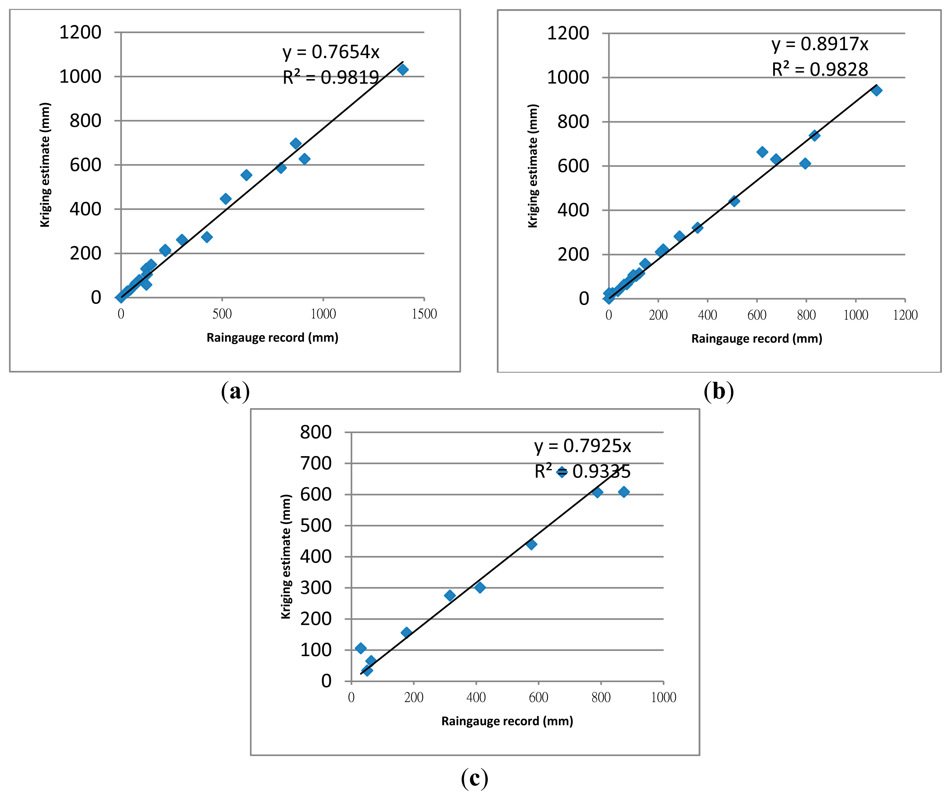
3.1. Validation of Kriging Estimates

Kriging was used in this study to estimate the rainfall at ungauged sites. However, how to validate the estimates using existing observation data becomes another important issue. The fitted parameters and kriging variance are listed in Table 3. From the basic statistical data in Table 1 and spatial distribution in Figure 2, the range of hourly, monthly, annual rainfall is quite large, the b sill parameter shows increase trend as the temporal scale enlarges; the a range parameter shows no significant variation except for six dry months. During six dry months, the rainfall regime dominated mainly by frontal rain lead to low rainfall intensity in winter and spring which yields wide influence range. Kriging variance in wet six months is far larger than that of dry six months, showing the significant rainfall amount distribution for dry (30%) and wet period (70%). Besides the 50 rain gauges, rainfall measurements of another three temporary rain gauge stations located in Xitou were used to validate the kriging estimates. By using the semi-variogram constructed from the 50 rain gauges, estimates of these three sites were then obtained and compared with actual point measurements. Monthly rainfall validations are shown in Figure 3. Although kriging results were underestimated by 11% to 24%, considering the high rainfall variability in mountainous areas, the correlation between estimates and measurements were high enough to be adjusted using simple regression.

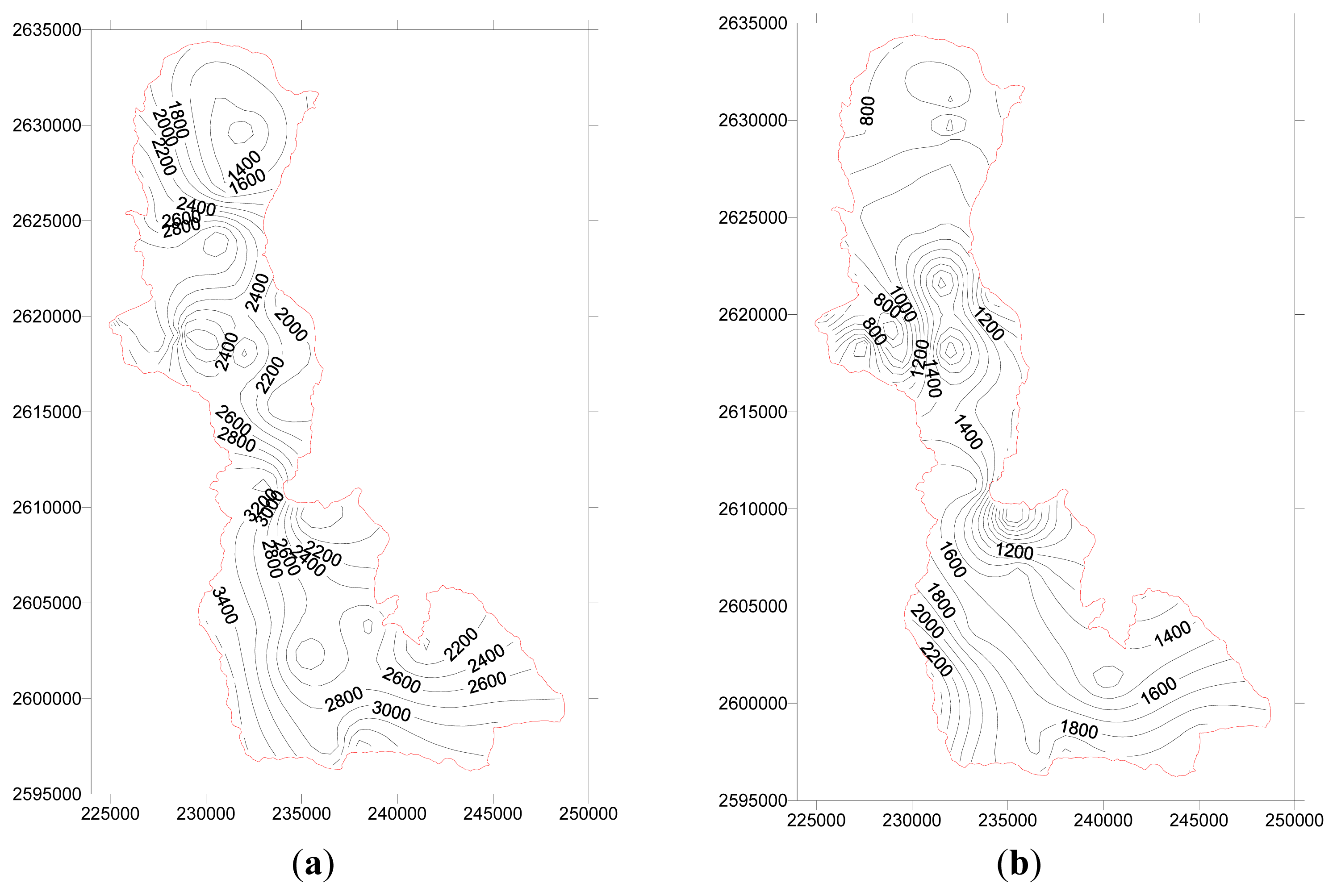
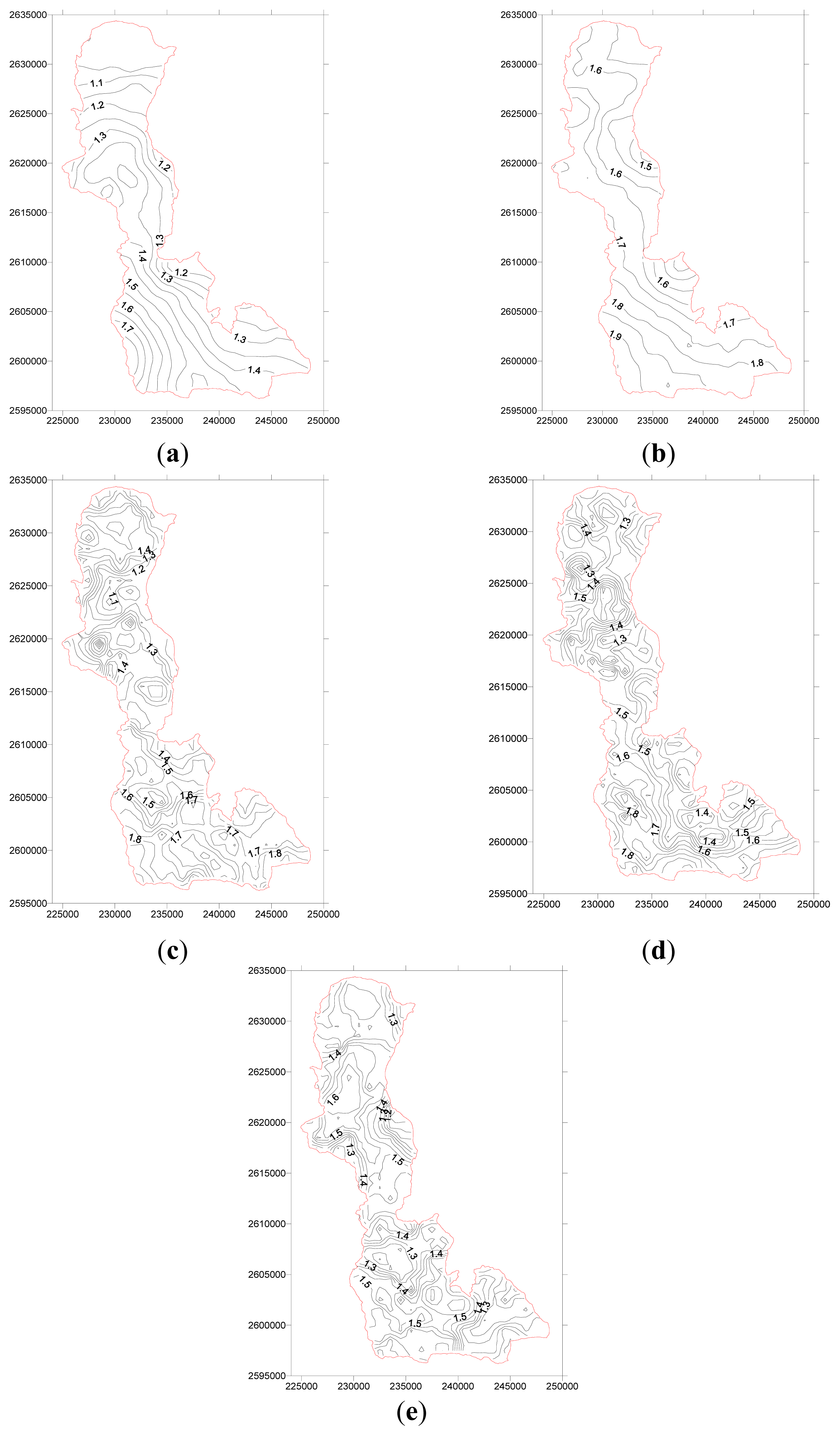
3.2. Uncertainty Distributed in Space

The entropy was used in this study to analyze the uncertainty of rainfall for individual gauges. The result shows the spatial distribution differs from typhoon hourly, monthly, six dry and wet monthly and annual rainfall, as illustrated in Figure 4. For hourly data, the contour line is comparably smooth, and the entropy values increase from north (1.05) to south (1.50) and east (1.35) to west (1.95). For monthly rainfall, the contour line changes locally, and the values are higher than those of typhoon hourly values, especially in northern and eastern areas, which indicates higher uncertainty exists in temporal scales. As aforementioned, the rainy season in the study area ranges from May to September, resulting in uneven monthly distribution. In addition, the entropy contour line of annual rainfall is irregularly distributed. However, the pattern of the annual contour map is distinct from the other two, revealing the larger local variation even with small entropy values. Compared with Figure 2a, around the rainfall center in Figure 4c, the contour line is also comparably smooth. This indicates that the entropy value in surrounding areas with large rainfall is smaller. If the network design is based on the uncertainty, the priority in this area is not so important, and vice versa.

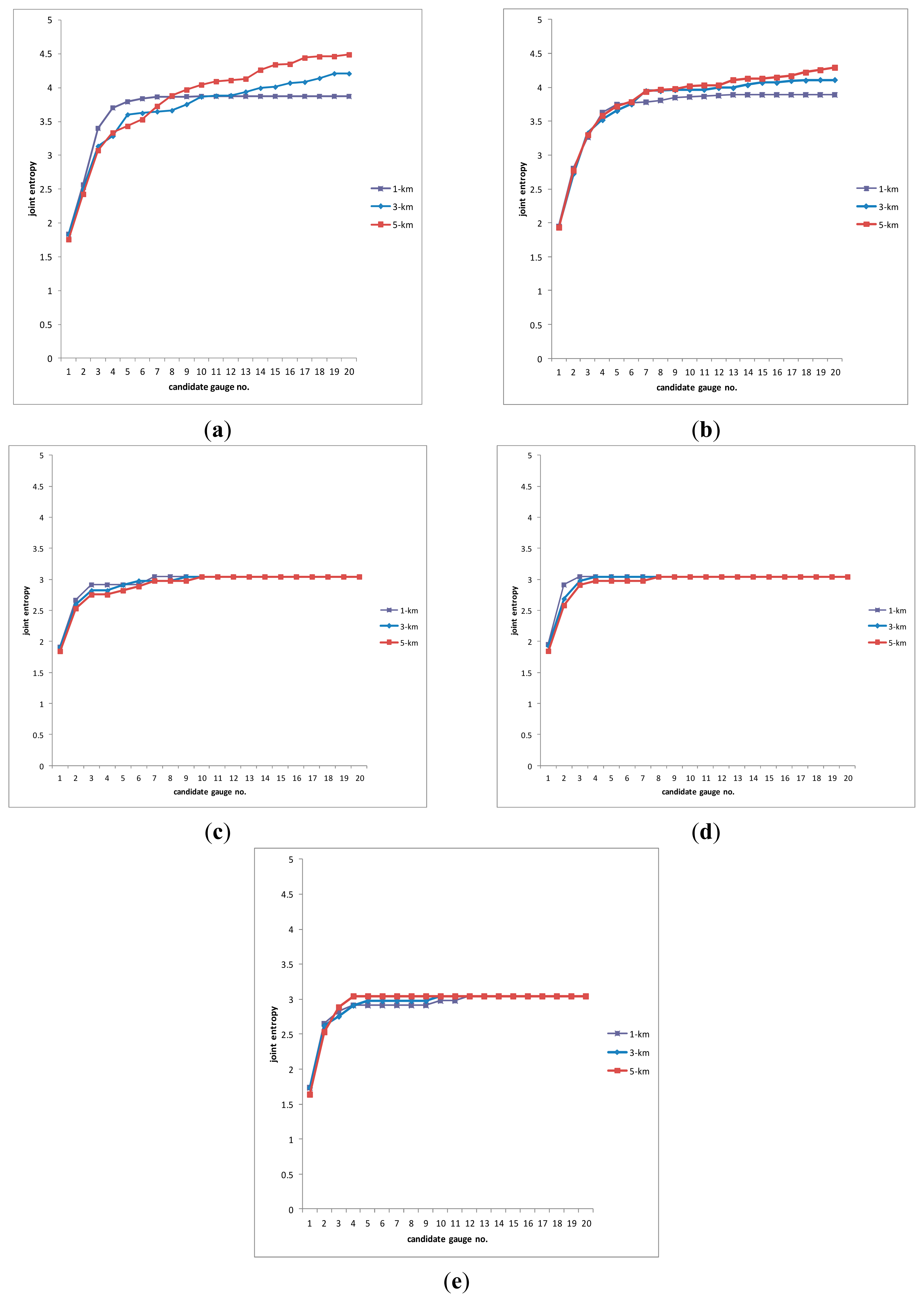
3.3 Spatial Scale Effect

If the same temporal scale was considered, the variation at the spatial scale is not so significant. The effect decreases as the temporal scale increases. Because of different candidate gauge stations for 1, 3 an 5-km, only the first 20 prioritized candidate rain gauge stations were compared for the spatial scale effect shown in Figure 5. For hourly data, the variation in the 5-km grid is larger than in the 3-km grid and in the 1-km grid. Before the eighth selected candidate rain gauge, the joint entropy value of 1-, 3-, and 5-km grid oscillates. However, the joint entropy of the 5-km grid is higher than that of 3-km grid and the 1-km gird after the eighth selected candidate rain gauges. The joint entropy of the 3-km grid is always higher than that of the 1-km grid. For the annual scale, no significant difference was found among the 1-, 3-, and 5-km grids. In general, for the first 20 prioritized candidate rain gauge stations, the maximum entropy of hourly, monthly, dry and wet six months and annual rainfall is around 4.5, 4.3, and 3.0, respectively. It implies the uncertainty of these two temporal scales are higher than the long-term scale and also implies that the spatial scale effect is less for long temporal scales and fewer rain gauges are required for long-term monitoring. In particular, the hourly data were collected during typhoon events, regarded as rainy and comparably large, and exhibiting diverse variability in high terrain relief. Within the 5-km grid, the joint entropy is larger because of more uncertainty existing in short-period rainfall. The rain gauge network is suggested to increase the number of stations to obtain more detailed variation for hydrologic design and rainfall forecasting.

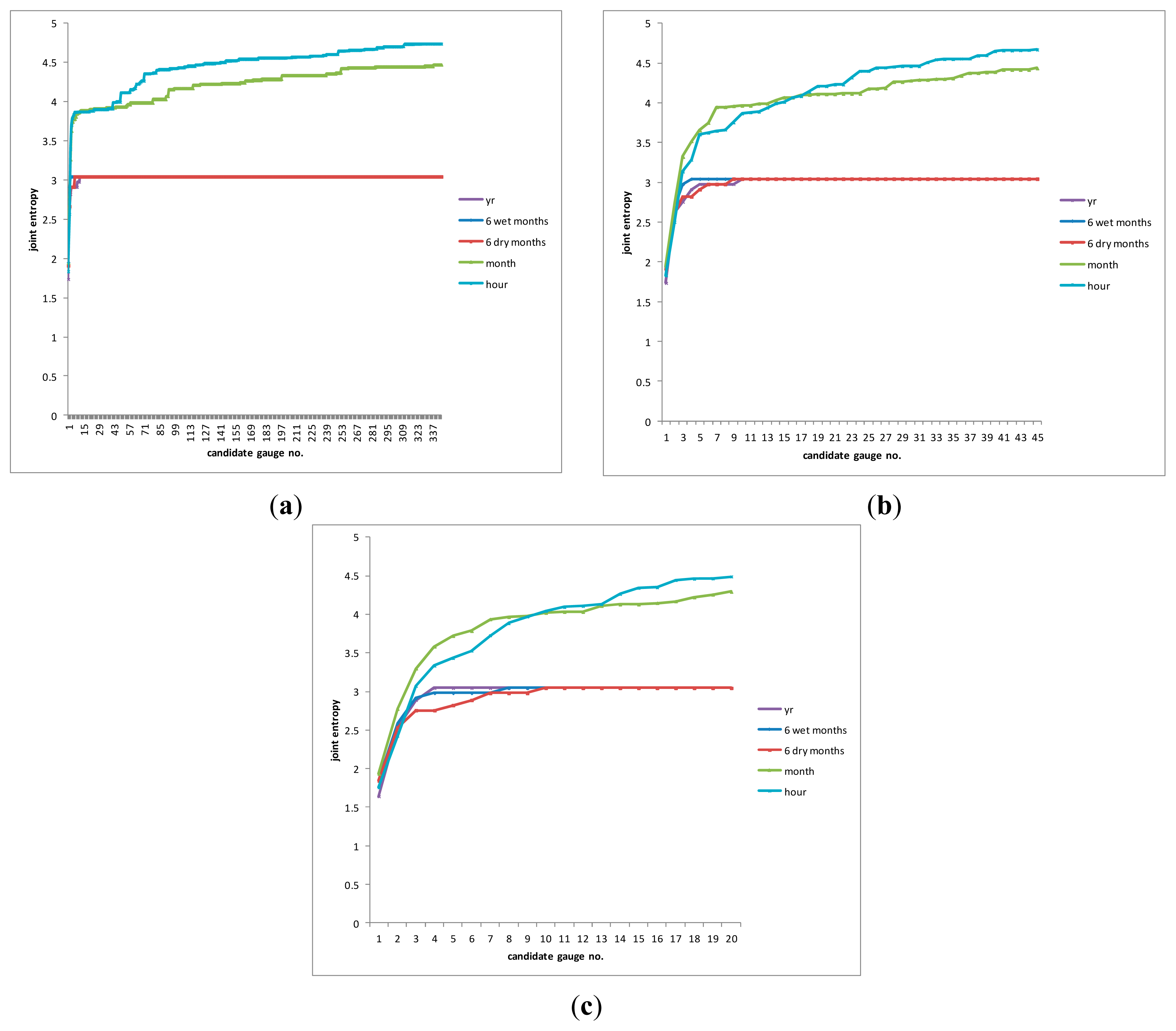
3.4. Temporal Scale Effect

Based on the same spatial scale, more candidate rain gauge stations are needed to reach the stable value of joint entropy for a short temporal scale. In Figure 6, fewer gauge stations are required to reach the stable value of joint entropy. The trends coincide with each other between different spatial scales. In the 5-km grid, only 4 stations are needed to reach maximum joint entropy, but more than 300 gauges are needed to reach maximum joint entropy in the 1-km grid. The maximum joint entropy value did not change much between the 1-, 3-, and 5-km grids, but that of the annual rainfall, dry and wet six months (around 3) is separated from hourly and monthly rainfall. The spatial scaling effect is also proved again not to be as significant at the temporal scale.

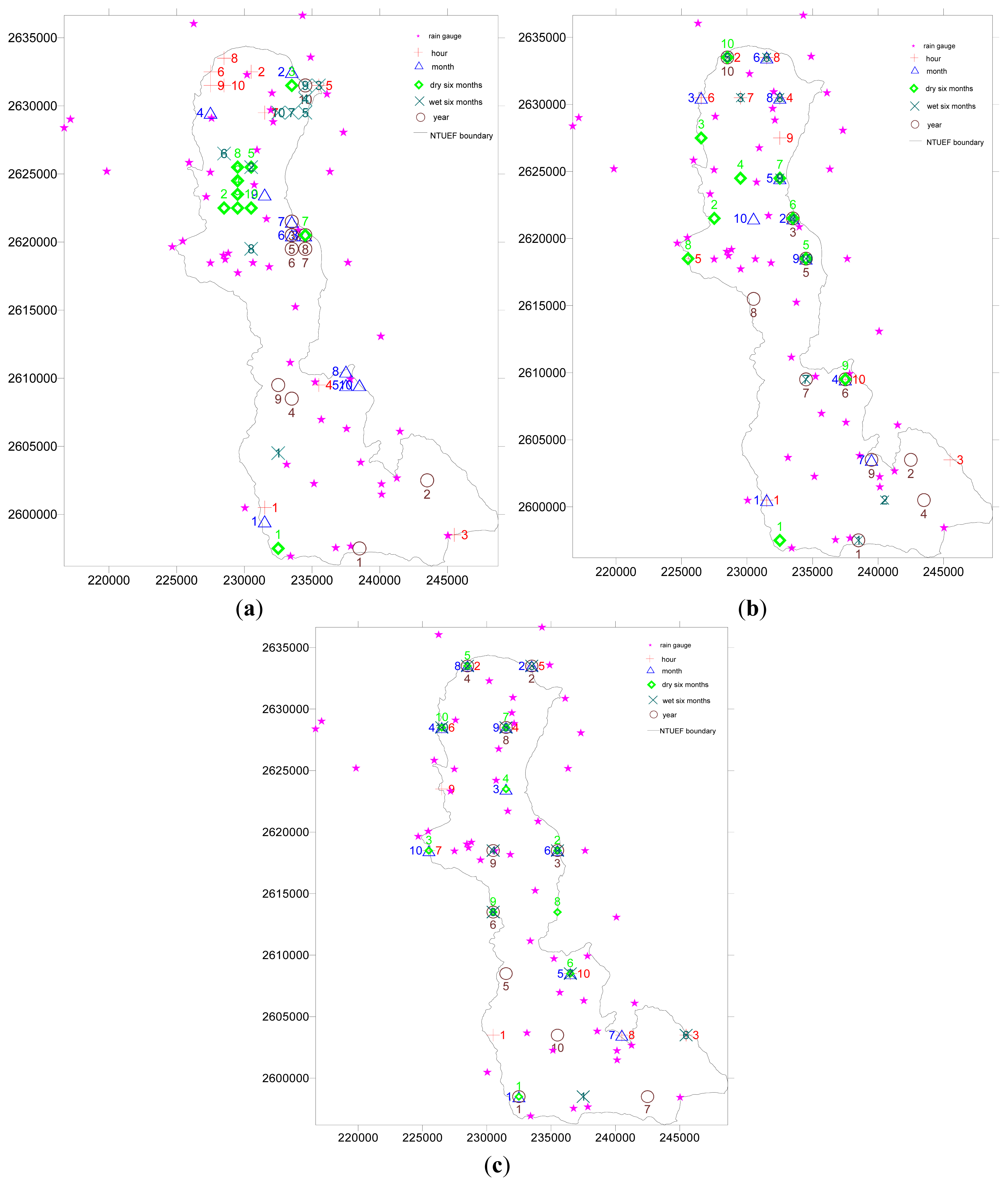
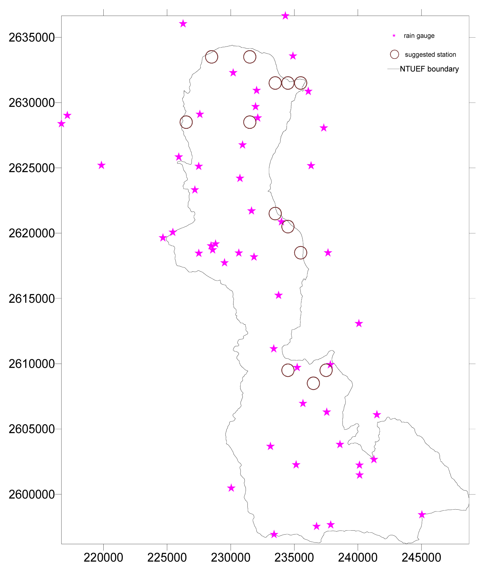
3.5. Optimal Rain Gauge Station Network of the NTUEF Area

The priorities of the rain gauge stations are determined by calculating the joint entropies of the study area. The priority of the rain gauge stations obtained on the basis of the entropy can also become the sequence of removal of the stations. As aforementioned, different candidate rain gauge stations exist for different spatial scales. The number and PRS are calculated to express the percentage of required gauge stations at the three spatial scales listed in Table 4. Figure 7 illustrates the first ten prioritized gauge stations in 1-, 3-, and 5-km grids. Figure 7a demonstrates the first prioritized candidate station almost located at the southwestern corner with all five temporal scales at the 1-km grid. Hourly, monthly and six dry months temporal scale are located around rain gauge No. 1. The annual rainfall around this region is over 3600 mm and also with the largest rainfall in the study area. However, the first prioritized candidate station for six wet months and annual temporal scale is located at rain gauge northern No.19 and eastern No.18, respectively. Three groups along the eastern boundary were clearly identified, implying that the existing rain gauge stations were crucial across temporal scales; however, no distinct groups were found in Figure 7b,c. More gauge stations are needed for these three concentrated groups. In addition, the second large prioritized candidate gauge stations were quite different across 1, 3, and 5 km. It can be inferred that the existing rain gauge stations not in the neighboring area of prioritized candidates should be addressed for the issue of stopping observation or abandonment. The decision for optimal rain gauge network can be made according to the prioritized and overlapped gauge stations across five temporal scales.
If the number of stations in the network is greater than the minimum number of candidate stations, then the stations exceeding the minimum candidate number can be processed for elimination. In Table 4, PRS exceeding the threshold value of 95% across different temporal scales is smaller at finer spatial scales. Although the entropy value changes in Figure 4e, only three to four gauges are enough to represent the variability of annual rainfall. The PRS of hourly, monthly, six dry and wet monthly and annual rainfall increases as the spatial scale enlarges. For the same spatial scale, the PRS for shorter temporal scale as hour and month is far larger than longer temporal scale; for the same temporal scale, the PRS increase as the spatial enlarges. It is noted the six rainy months need less candidate stations than six dry months which implies more variation and uncertainty of rainfall existed during dry seasons. According to the third category for the WMO standard aforementioned, the study area of 327.86 km2 is equivalent to 13.1 gauges, very close to the number analyzed for hourly and monthly rainfall in the 5-km grid in Table 4. More rainfall information can be obtained as the required rain gauges increased for 3- and 1-km scale. However, for efficiency, 13 and 14 candidate stations at monthly and hourly at the 5-km grid, equivalent to one-fourth of existing rain gauge stations, are enough for general use, respectively; for hydrologic design and using the prioritized network at 3- or 1-km grid, the number will double or even more. Compromising the accuracy and network density, 13 candidate stations were identified as the optimal network according to the prioritized and overlapped gauge stations across all spatiotemporal scales in Figure 8.
Compared with Figure 7, these 13 candidate stations locate very closely with three concentrated groups found at 1-km scale. Kay and Kutiel [46] suggested a new approach in mapping climate maps of precipitation and found the actual rainfall field is more closely represented if more rainfall events and dense grid. In this study, the 1-km grid can capture more rainfall uncertainty than 3- and 5-km grid but with low PRS, indicating more candidate rain stations need to yield same accuracy. Kutiel and Kay [47] found no consistent recommendation of network design is best for all purposes. From Table 4 we demonstrate the PRS for fifteen combination of spatiotemporal scale, for best efficiency and low cost of rain gauge configuration, we should choose lowest PRS both at spatial and temporal scale, which means 1-km at six months or annual scale is best choice. However, it may only satisfy the evaluation or research for long-term climate and fail to capture need information for short-term such as hydrologic forecast.
The authors did not analyze all the hourly rainfall records for three reasons. First, for hydrologic design and disaster warning and prevention, the records with “rain” are far more important than “no-rain.” Second, if all the hourly data are considered, the sample size will be larger than 183,000, which contains too many zeros or tiny rain records (e.g., 0.5 mm). The discrete distribution of data will cause the bias in calculating the entropy with respect to monthly and annual data in Equation (2). Third, the rainfall of typhoon events covered most of the study area for constructing semi-variogram in Equation (1), preventing inadequate semi-variogram resulting from rainfall only in some local areas. Despite above three reasons, hourly data analyzed in this study is still part of the whole dataset and just represent the network design for rainy hours. For No. 1 rain gauge (Alishan), there were only about half rainy days between 1992 and 2012 (total 7671 days).We do not include daily rainfall data for the same reasons even though it may be a suitable temporal scale between hour and month. Compared with the work by Cheng et al. [5] at hourly and annual scale, this study only includes hourly data for typhoons with the selecting criterion that over two thirds records are non-zero data, we neglected the other three major rainfall types, i.e., convective, Mei-Yu and frontal rain. The major reason is the rain intensity of seven typhoon events in study area is large enough to represent the extreme rainfall condition in study area, in particular, the Typhoon Morakot in Aug 2009. From Table 1, 30% rain gague stations (15 out of 50) its maximum hourly rainfall had reached 100 mm. The hourly spatial variability with annual rainfall is not significant different as the aforementioned study may lead to different area size 2200 km2, rain gauge number 27, with respect to 328 km2 and 50 in this study.

4. Conclusions

The proposed model can be used to design an optimal rainfall network that provides the majority of rainfall information as the existing rainfall network. Derived from the data of the existing rainfall network, it is used to analyze the spatiotemporal scaling effect and suggest an optimal candidate station network by use of information entropy and kriging. In this study, we demonstrated that the candidate rainfall network is able to reduce the number of rain gauge stations, while accurately reflecting the location of precipitation. The results indicate that the optimal rainfall network at different combinations of spatiotemporal scales consists of candidate stations with capacities to provide 95% rainfall information of existed rain gauge stations. The relevant conclusions and propositions are as follows:
(1)
It exhibits different locations for first prioritized candidate rain gauges between spatiotemporal scales.
(2)
The effect of spatial scales is insignificant in comparison to temporal scales for network design. From the joint entropy value, the difference between hourly and monthly scales is more significant than the six dry, wet months and annual rainfall. However, the difference is significant across the spatial scale.
(3)
A smaller number and a lower percentage of required stations (PRS) are needed to reach stable joint entropy of long duration (six months or year) at finer spatial scale. Compromising the accuracy and network density, we suggest the optimal network design comprising of 13 candidate stations be suitable across all spatiotemporal scales.

Acknowledgments

This paper is based on the follow-on work supported by research project of the National Taiwan University Experimental Forest, Taiwan (NTUEF 2006-B06 and 2009-A05) and partial-financially support of Project no. MOST 103-2119-M-002-018- grant by Ministry of Science and Technology of Taiwan. In addition, special thanks go to the lab led by Hsin-Hsiung Chen for providing the rainfall data of three additional rain gauges.

Author Contributions

Chiang Wei was responsible for the research framework and managed the manuscript. Hui-Chung Yeh took charge of the code programming and data analysis. Yen-Chang Chen assisted with building the framework and conducting data analysis. All authors have read and approved the final manuscript.

Conflicts of Interest

The authors declare no conflict of interest.

References

  1. Hackett, O.M. National water data program. J. Am. Water Work Assoc 1966, 58, 786–792. [Google Scholar]
  2. Campbell, S.A. Sampling and Analysis of Rain; American Society of Testing and Materials: West Conshohocken, PA, USA, 1983. [Google Scholar]
  3. World Meteorological Organisation (WMO), Guide to Hydrometeorological Practices; WMO Technical Paper 82; WMO: Geneva, Switzerland, 1970.
  4. Markus, M.H.; Knapp, V.; Tasker, G.D. Entropy and generalized least square methods in assessment of the regional value of streamgauges. J. Hydrol 2003, 283, 107–121. [Google Scholar]
  5. Cheng, K.S.; Lin, Y.C.; Liou, J.J. Rain-gauge network evaluation and augmentation using geostatistics. Hydrol. Process 2008, 22, 2554–2564. [Google Scholar]
  6. Harmancioglu, N. Measuring the information content of hydrological processes by the entropy concept. J. Civ. Eng. Facul. Ege Univ 1981, 13–40. [Google Scholar]
  7. Awumah, K.; Goulter, I. Assessment of reliability in water distribution networks using entropy based measures. Stoch. Hydrol. Hydraul 1990, 4, 309–320. [Google Scholar]
  8. Awumah, K.; Goulter, I.; Bhatt, S.K. Entropy-based redundancy measures in water-distribution networks. J. Hydraul. Eng 1991, 117, 595–614. [Google Scholar]
  9. Krstanovic, P.F.; Singh, V.P. Evaluation of rainfall network using entropy II: Application. Water Resour. Manag 1992, 6, 295–314. [Google Scholar]
  10. Al-Zahrani, M.; Husain, T. An algorithm for designing a precipitation network in the southwestern region of Saudi Arabia. J. Hydrol 1998, 205, 205–216. [Google Scholar]
  11. Ozkul, D.S.; Harmancioglu, N.B.; Singh, V.P. Entropy-based assessment of water quality monitoring networks. J. Hydraul. Eng 2000, 5, 90–100. [Google Scholar]
  12. Mogheir, Y.; Singh, V.P. Application of information theory to groundwater quality monitoring networks. Water Resour. Manag 2002, 16, 37–49. [Google Scholar]
  13. Mogheir, Y.; de Lima, J.L.M.P.; Singh, V.P. Characterizing the spatial variability of groundwater quality using the entropy theory: I. Synthetic data. Hydrol. Process 2004, 18, 2165–2179. [Google Scholar]
  14. Nunes, L.M.; Cunha, M.C.; Ribeiro, L. Groundwater Monitoring Network Optimization with Redundancy Reduction. J. Water Resour. Plann. Manag 2004, 130, 33–43. [Google Scholar]
  15. Masoumi, F.; Kerachian, R. Assessment of the groundwater salinity monitoring network of the Tehran region: Application of the discrete entropy theory. Water Sci. Technol 2008, 58, 765–771. [Google Scholar]
  16. Mogheir, Y.; Singh, V.P.; de Lima, J.L.M.P. Spatial assessment and redesign of a groundwater quality monitoring network quality using entropy theory, Gaza Strip, Palestine. Hydrogeol. J 2006, 14, 700–712. [Google Scholar]
  17. Yoo, C.; Jung, K.; Lee, J. Evaluation of rain gauge network using entropy theory: Comparison of mixed and continuous distribution function applications. J. Hydrol. Eng 2008, 13, 226–235. [Google Scholar]
  18. Mogheir, Y.; de Lima, J.L.M.P.; Singh, V.P. Entropy and multi-objective based approach for groundwater quality monitoring network assessment and redesign. Water Resour. Manag 2009, 23, 1603–1620. [Google Scholar]
  19. Alfonso, L.; Lobbreche, A.; Price, R. Information theory-based approach for location of monitoring water level gauges in polder. Water Resour. Res 2010, 46, W03528. [Google Scholar]
  20. Alfonso, L.; Lobbrecht, A.; Price, R. Optimization of water level monitoring network in polder systems using information theory. Water Resour. Res 2010, 46, W12553. [Google Scholar]
  21. Li, C.; Singh, V.P.; Mishra, A.K. Entropy theory-based criterion for hydrometric network evaluation and design: Maximum information minimum redundancy. Water Resour. Res 2012, 48, W5521. [Google Scholar]
  22. Gong, W.; Gupta, H.V.; Yang, D.W.; Sricharan, K.; Hero, A.O. Estimating epistemic and aleatory uncertainty during hydrologic modeling: An information theoretic approach. Water Resour. Res 2013, 49, 2253–2273. [Google Scholar]
  23. Chen, Y.C.; Wei, C.; Yeh, H.C. Rainfall network design using kriging and entropy. Hydrol. Process 2008, 22, 340–346. [Google Scholar]
  24. Yeh, H.C.; Chen, Y.C.; Wei, C.; Chen, R.H. Entropy and Kriging Approach to Rainfall Network Design. Paddy Water Environ 2011, 9, 343–355. [Google Scholar]
  25. Awadallah, A.G. Selecting optimum locations of rainfall stations using kriging and entropy. Int. J. Civil Environ. Eng 2012, 12, 36–41. [Google Scholar]
  26. Amorocho, J.; Espildora, B. Entropy in the assessment of uncertainty in hydrologic systems and models. Water Resour. Res 1973, 9, 1511–1522. [Google Scholar]
  27. Chapman, T.G. Entropy as a measure of hydrologic data uncertainty and model performance. J. Hydrol 1986, 85, 111–126. [Google Scholar]
  28. Harmancioglu, N.; Yevjevich, V. Transfer of hydrologic information among river points. J. Hydrol 1987, 91, 103–118. [Google Scholar]
  29. Yang, Y.; Burn, D.H. An entropy approach to data collection network design. J. Hydrol 1994, 157, 307–324. [Google Scholar]
  30. Singh, V.P. The Use of Entropy in Hydrology and Water Resources. Hydrol. Process 1997, 11, 587–626. [Google Scholar]
  31. Kawachi, T.; Maruyama, T.; Singh, V.P. Rainfall entropy for delineation of water resources zones in Japan. J. Hydrol 2001, 246, 36–44. [Google Scholar]
  32. Mishra, A.K.; Coulibaly, P. Hydrometric network evaluation for Canadian watersheds. J. Hydrol 2010, 380, 420–437. [Google Scholar]
  33. Memarzadeh, M.; Mahjouri, N.; Kerachian, R. Evaluating sampling locations in river water quality monitoring networks: Application of dynamic factor analysis and discrete entropy theory. Environ. Earth Sci 2013, 70, 2577–2585. [Google Scholar]
  34. Sivapalan, M.; Grayson, R.; Woods, R. Preface Scale and scaling in hydrology. Hydrol. Process 2004, 18, 1369–1371. [Google Scholar]
  35. Viney, N.R.; Sivapala, M. A framework for scaling of hydrologic conceptualizations based on a disaggregation–aggregation approach. Hydrol. Process 2004, 18, 1395–1408. [Google Scholar]
  36. Serra, Y.L.; Mcphaden, M.J. Multiple Time- and Space-Scale Comparisons of ATLAS Buoy Rain Gauge Measurements with TRMM Satellite Precipitation Measurements. J. Appl. Meteorol 2003, 42, 1045–1059. [Google Scholar]
  37. Singh, V.P. Entropy Theory and Its Application in Environmental and Water Engineering; John Wiley & Sons: Hoboken, NJ, USA, 2013. [Google Scholar]
  38. Stewart, J.B.; Engman, E.T.; Feddes, R.A.; Kerr, Y. Scaling up in Hydrology Using Remote Sensing; John Wiley & Sons: Hoboken, NJ, USA, 1996. [Google Scholar]
  39. Matheron, G. Traite De Geostatistique Appliqué, Tome 1; Editions Technip: Paris, France, 1962. (In French) [Google Scholar]
  40. Rodriguez-Iturbe, I.; Sanabria, M.G.; Bras, R.L. A geomorphoclimatic theory of the instantaneous unit hydrograph. Water Resour. Res 1982, 18, 877–886. [Google Scholar]
  41. Chiles, J.-P.D.P. Geostatistics-Modeling Spatial Uncertainty; Willey: New York, NY, USA, 1999. [Google Scholar]
  42. Wackernagel, H. Multivariate Geostatistics; Springer-Verlag: Berlin, Germany, 2003. [Google Scholar]
  43. Kebaili, B.Z.; Chebbi, A. Comparison of two kriging interpolation methods applied to spatiotemporal rainfall. J. Hydrol 2009, 365, 56–73. [Google Scholar]
  44. Shannon, C.E. A mathematical theory of communication. Bell Syst. Tech. J 1948, 27, 623–656. [Google Scholar]
  45. Shannon, C.E.; Weaver, W. Mathematical Theory of Communication; University of Illinois Press: Champaign, IL, USA, 1949. [Google Scholar]
  46. Kay, P.A.; Kutiel, H. Some remarks on climatic maps of precipitation. Clim. Res 1994, 4, 233–241. [Google Scholar]
  47. Kutiel, H.; Kay, P.A. Effects of network design on climatic maps of precipitation. Clim. Res 1996, 7, 1–10. [Google Scholar]
Figure 1. Candidate and existing rain gauges in the study area NTUEF.
Entropy 16 04626f1
Figure 2. Contour maps of (a) average annual rainfall between 1992 and 2012; and (b) Typhoon Morakot rainfall of 5–9 August 2009 at the NTUEF area.
Entropy 16 04626f2
Figure 3. Validation of monthly rainfall at three stations in Xitou Tract by Ordinary Kriging; (a) Phoenix 3.8 K Station (January 2004 to September 2005); (b) Liu Long Gully Station (January 2004 to September 2005); and (c) Upper Station of University Gully (December 2004 to September 2005).
Entropy 16 04626f3
Figure 4. Entropy contour maps at (a) hourly; (b) monthly; (c) six dry monthly; (d) six wet monthly; and (e) annual scale.
Entropy 16 04626f4
Figure 5. Variation of joint entropy for first 20 prioritized candidate gauges at (a) hourly, (b) monthly; (c) six dry monthly; (d) six wet monthly; and (e) annual scale.
Entropy 16 04626f5
Figure 6. Variation of joint entropy vs. candidate gauge number for (a) 1-km scale; (b) 3-km scale; (c) 5-km scale.
Entropy 16 04626f6
Figure 7. First 10 prioritized candidate gauges in the study area at (a) 1-km scale; (b) 3-km scale; and (c) 5-km scale at different temporal scales.
Entropy 16 04626f7
Figure 8. Locations of 13 suggested rain gauge candidates.
Entropy 16 04626f8
Table 1. Summary description of rain gauge stations in Study Area.
No.Rain Gauge StationElevation (m)TM2 (m)Hourly Rainfall for Typhoon Events (mm)Monthly Rainfall (mm)Annual Rainfall (mm)
EastingNorthingMaximumMinimumMeanStandard DeviationMaximumMinimumMeanStandard DeviationMaximumMinimumMeanStandard Deviation
1AliShan2,413230,0432,600,476123.00.025.825.63,346.00.0336.6438.15,886.72,196.54,039.21,140.9
2Mt. Jade3,845245,0302,598,43564.00.014.713.42,189.90.0254.8299.04,705.21,702.73,058.2830.3
3Xitou Nursery1,169228,5832,618,722110.00.017.020.61,770.00.0202.3246.14,053.01,291.02,455.3673.5
4Jushan-NTU156216,6932,628,383145.00.010.218.11,173.00.0181.0214.82,821.61,355.12,221.0449.4
5Shueli-NTU295234,8932,633,571123.50.010.517.21,512.50.0150.7200.42,816.02,12.51,835.9724.6
6Nemoupu-NTU509233,9872,620,868125.50.011.215.81,008.00.0153.3175.42,805.0946.01,820.9491.0
7Heshe-NTU780237,8302,609,92074.00.011.214.31,258.00.0154.2185.02,688.51,062.01,855.9498.8
8Chinshueigao-NTU520227,5762,629,098100.00.09.214.51,271.60.0187.6222.14,275.0680.52,234.6852.4
9Hsingouko2,540236,7492,597,543112.50.016.815.92,203.00.0241.7294.04,524.5787.02,828.71,068.2
10Dann1,528224,6722,619,64675.50.08.611.2945.00.0180.7197.93,154.0773.02,088.8627.1
11Jushan151217,1572,629,012170.00.08.916.91,133.50.0177.6207.33,205.0613.02,047.8611.7
12Wanshian2,403240,0802,613,07585.00.012.815.01,633.50.0208.3247.93,642.0924.02,421.6832.5
13Phoenix Garden878227,4852,625,117141.00.011.918.41,292.00.0218.2235.63,671.0948.02,522.5741.5
14Xitou Observation1,771229,5142,617,73161.00.09.29.61,053.50.0192.8203.23,139.0909.52,219.5629.0
15Long-Shen Bridge339236,1002,630,858130.50.09.015.0900.00.0164.5179.42,812.51,133.51,921.2653.3
16Ji-Ji235226,2572,636,039103.50.08.313.2975.00.0188.7210.03,100.51,504.52,256.7923.4
17GuanShan1,780240,1352,601,47281.50.014.815.41,171.50.0227.7225.23,695.91,296.52,444.9820.9
18Pasture2,677237,8602,597,660136.00.018.317.42,383.50.0304.1387.75,218.81,653.53,719.51,025.3
19Shenmu Village1,595233,1252,603,66891.50.016.417.02,141.50.0260.1330.54,649.51,653.53,114.41,664.2
20Chungshinlun661219,8392,625,19263.50.09.412.61,075.00.0231.0264.03,682.01,554.52,731.81,468.3
21Shueli593234,2952,636,644110.00.010.217.5911.00.0193.9218.33,094.01,451.02,341.81,276.9
22Fongchiou1,151237,6472,618,49184.50.011.114.31,211.00.0166.9210.12,938.01,088.02,021.51,114.5
23ShangAn781236,3212,625,16766.00.08.612.2804.50.0162.0190.12,914.01,193.01,973.31,074.3
24Hsin-shin Bridge897235,6802,606,95796.50.014.217.21,751.50.0193.9266.13,277.51,291.02,425.11,297.9
25Dongpu887241,4932,606,09167.00.010.211.81,307.00.0169.6219.22,917.01,107.02,092.91,138.7
26Siluang1,001237,3152,628,05878.50.010.715.5963.50.0186.7217.33,061.01,313.52,193.81,218.5
27Xitou office1,156228,4532,619,02856.00.013.512.91,218.50.0223.2277.44,005.51,125.53,053.31,369.3
28TienDi787230,7282,624,19953.50.011.312.61,360.50.0140.3266.43,122.5137.02,326.5973.3
29GuangHsin645225,9172,625,83149.50.09.812.21,190.50.0238.9286.93,628.5329.03,124.51,299.3
30No.3 Gully1,185228,8112,619,17425.00.04.25.7776.00.0167.2180.23,339.5712.51,937.0907.2
31Neihu elementary school772227,1812,623,31652.00.09.811.71,214.50.0201.6258.73,560.5901.03,090.31,157.6
32Lower University Gully1,197227,4922,618,456106.00.015.116.81,663.00.5255.6402.73,956.0222.53,334.21,207.7
33Wushio1,495225,4502,620,06432.00.07.37.52,296.50.0212.4394.33,941.0610.03,400.81,221.4
34Yashanpin1,390233,3832,611,14486.00.017.519.41,872.50.0269.3367.14,221.02,264.53,534.01,478.1
35Alibudon1,208235,2272,609,71231.50.04.87.9823.50.0135.8162.12,876.0530.51,549.0780.0
36Salishian1,216241,2592,602,66461.50.010.312.31,211.50.0208.0274.33,284.5824.51,941.2799.8
37Neuchangpin1,306237,5492,606,29283.00.013.816.51,500.00.0185.3247.92,672.51,768.52,302.81,008.6
38Shenmu1,315235,1422,602,25975.00.012.915.51,490.50.5297.5413.53,885.0425.02,185.3955.8
3932-compartment1,823240,1232,602,23159.00.015.613.51,714.50.0223.5298.93,073.02,050.52,318.01,157.2
4030-compartment2,097238,5882,603,81466.00.014.814.41,725.00.0227.2341.34,294.01,134.52,903.71,244.7
4129-compartment2,298233,4082,596,92480.50.020.220.72,307.50.0347.0466.65,450.5974.53,453.31,774.8
4220-compartment967233,7652,615,24172.00.012.815.11,372.515.0174.8282.12,010.0603.01,456.5573.6
4321-compartment1,280231,8322,618,17499.50.022.324.42,243.57.0296.3433.42,946.02,048.52,518.51,023.4
4422-compartment892230,6362,618,47579.00.013.717.11,403.03.0198.1259.82,859.51,859.52,129.6877.4
4524-compartment1,278231,6352,621,701107.00.018.921.22,042.00.0171.1339.82,820.5442.01,582.8797.0
4613-compartment454231,9532,629,68651.50.07.911.0708.58.5178.2193.92,728.51,003.51,870.9804.6
4716-compartment1,002232,0382,630,93271.00.010.614.9303.02.5114.4203.51,473.5508.51,058.4458.3
4817-compartment454230,1942,632,28351.00.08.910.4343.00.0166.6259.31,403.0409.51,110.8300.3
4911-compartment1,228230,9312,626,75760.00.012.914.5915.021.0216.6207.22,998.01,402.02,219.9929.7
509-compartment1,213232,1272,628,82357.00.010.412.3755.021.5216.4189.22,391.51,301.51,839.6762.0
Table 2. Typhoon events in this study between 1996 and 2012.
TyphoonDateMaximum Wind (m/s)Rainfall Duration (h)Damage (Billion, NT)
Herb29 July–1 August 1996534439.3
Toraji28–31 July 2001382414.7
Mindulle28 June–3 July 200445726.5
Kalmeigi16–18 July 200833323.4
Silaku11–16 September 200851755.6
Marakot5–10 August 2009409647.7
Saola30 July–3 August 2012384216.2
Table 3. Details of kriging estimates.
Temporal Scaleb (Sill, mm2)a (Range Parameter, m)Kriging Variance (mm2)
Hour165 ± 29240,243 ± 25,53821 ± 62
Month23,529 ± 67,31639,481 ± 67,3163,154 ± 7,760
Dry six months43,209 ± 52,81350,926 ± 22,7083,198 ± 4,184
Wet six months583,324 ± 560,41039,499 ± 27,17164,250 ± 58,808
Annual645,623 ± 654,17531,337 ± 29,685104,080 ± 107,613
Table 4. Number and Percentage of Required Stations (PRS) at different spatiotemporal scales.
ScaleCandidate Station NumberHourMonthSix Dry MonthsSix Wet MonthsYear
1-km346126 (36.4%)143 (41.3%)3(0.9%)2(0.6%)4 (1.1%)
3-km4526 (57.8%)28 (62.2%)5(11.1%)3(6.7%)4 (8.9%)
5-km2014 (70.0%)13 (65.0%)6(30%)3(15%)3 (15.0%)

