Entropy Production in Pipeline Flow of Dispersions of Water in Oil

Department of Chemical Engineering, University of Waterloo, Waterloo, ON N2L 3G1, Canada
Entropy 2014, 16(8), 4648-4661; https://doi.org/10.3390/e16084648
Submission received: 23 July 2014
/
Revised: 4 August 2014
/
Accepted: 15 August 2014
/
Published: 19 August 2014
(This article belongs to the Section Thermodynamics)
Abstract
:Entropy production in pipeline adiabatic flow of water-in-oil emulsions is investigated experimentally in three different diameter pipes. The dispersed-phase (water droplets) concentration of emulsion is varied from 0 to 41% vol. The entropy production rates in emulsion flow are compared with the values expected in single-phase flow of Newtonian fluids with the same properties (viscosity and density). While in the laminar regime the entropy production rates in emulsion flow can be described adequately by the single-phase Newtonian equations, a significant deviation from single-phase flow behavior is observed in the turbulent regime. In the turbulent regime, the entropy production rates in emulsion flow are found to be substantially smaller than those expected on the basis of single-phase equations. For example, the entropy production rate in water-in-oil emulsion flow at a dispersed-phase volume fraction of 0.41 is only 38.4% of that observed in flow of a single-phase Newtonian fluid with the same viscosity and density, when comparison is made at a Reynolds number of 4000. Thus emulsion flow in pipelines is more efficient thermodynamically than single-phase Newtonian flow.
PACS Codes: 5; 47; 82
1. Introduction
In the design and analysis of practical processes, it is important to determine how efficiently energy is utilized. As many processes consist of a number of steps, it is often necessary to carry out thermodynamic analysis of each step and to determine the extent to which energy is wasted or dissipated in each step due to irreversibilities in the process.
The amount of energy wasted or work lost as a result of irreversibilities is directly related to entropy production in the process. It is well known that [1,2]:
where Ẇlost is the rate of lost work, To is the surroundings temperature, and ṠG is the total rate of entropy generation due to internal (within control volume) and external (outside the control volume) irreversibilities. According to the second law of thermodynamics, ṠG >0 for any irreversible process. ṠG = 0 only when the process is completely reversible (no internal and external irreversibilities). The importance of Equation (1) is aptly described by the following statement of Smith et al. [1] “The engineering significance of this result is clear. The greater the irreversibility of a process, the greater the rate of entropy production and the greater the amount of energy that becomes unavailable for work. Thus every irreversibility carries with it a price.”
Another equivalent form of Equation (1) is as follows [3]:
where ψ̇destruction is the total rate of exergy destruction. The thermo-mechanical exergy associated with a fluid stream per unit mass is given as follows:
where h and s are specific enthalpy and specific entropy of fluid, respectively, ho and so are specific enthalpy and specific entropy of fluid in dead state, respectively, V is fluid velocity, g is acceleration due to gravity, and z is elevation of the fluid stream with respect to the dead state. According to the second law of thermodynamics, ψ̇destruction > 0 for any irreversible process. Thus irreversibilities in a process cause production of entropy and destruction of exergy.
In a multi-step process, it is important to estimate the rate of entropy generation in each step and compare the values of different steps to identify the process steps where irreversibilities are high. To that end, it is useful to compare the ratio ṠG,step/∑ṠG for different steps.
This article is related to entropy production in flow of dispersions of oil and water. Dispersions of droplets of one liquid distributed in another immiscible liquid (continuous phase), also called emulsions, are encountered in a variety of engineering applications and systems [4–9]. Emulsions can be classified into two broad groups: (a) water-in-oil (designated as W/O) emulsions, and (b) oil-in-water (designated as O/W) emulsions. The water-in-oil emulsions consist of water droplets dispersed in a continuum of oil phase whereas the oil-in-water emulsions have a reverse arrangement; i.e., oil droplets are dispersed in a continuum of water phase. A significant portion of the world crude oil is produced in the form of emulsions. Large quantities of emulsion-based fluids are also used for oil-well drilling, as well as for fracturing and acidizing purposes. In some situations where the crude oil being produced from a given oil well is highly viscous in nature, water is often injected into the production well bore to convert the high viscosity oil to a low viscosity oil-in-water emulsion. Another important application of emulsions in the petroleum industry involves the transportation of highly viscous crude oils in the form of oil-in-water emulsions. To transport the highly viscous crude oils (such as bitumen and heavy oils) via pipelines, it is necessary to either heat the oil to reduce its viscosity or dilute the oil with a low viscosity hydrocarbon diluent. In the former case, heating cost and pipeline insulation costs are usually very high. In the latter case, the cost of diluent and its availability pose difficult problems. These problems, however, can be avoided if the crude oil is transported in the form of an oil-in-water emulsion. The viscosity of oil-in-water emulsions is in general very low compared with the crude oil. Interest has also been shown on the use of emulsions to displace oil in the secondary oil recovery processes. Emulsions are also being considered as blocking agents to control the permeability of the formation.
The applications of emulsions in industries other than petroleum are numerous [4]. Many products of commercial importance are sold in emulsion form. Several books have been written describing the commercial applications of emulsion systems. The nonpetroleum industries where emulsions are of considerable importance include food, medical and pharmaceutical, cosmetics, agriculture, explosives, polishes, leather, textile, bitumen, paints, lubricants, polymer, and transport.
In a majority of the applications of emulsions just mentioned, flow of emulsions in pipelines and other process equipment is commonly encountered. Thus it is of practical significance to know the rate of entropy production in pipeline flow of emulsions. The main objective of this work is to experimentally investigate the production of entropy in pipeline flow of water-in-oil emulsions consisting of water droplets dispersed in a continuum of oil.
It should be pointed out that a number of research articles have been published on concurrent flow of oil and water in pipelines in the past. The research work carried out on this subject (simultaneous flow of oil and water in pipes) can be classified into four groups: (a) phase-inversion in oil-water pipe flows [10–15]; (b) droplet size and droplet size distribution in oil-water dispersed flows in pipes [16–19]; (c) flow patterns/maps in oil-water pipe flows [20–23]; and (d) pressure drop in oil-water pipe flows [6,24–26]. To our knowledge, little or no attention has been given to the second law analysis and entropy production in pipeline flow of oil and water dispersions.
2. Theoretical Background
Consider a control volume with one inlet and one outlet. Let the rate of heat transfer from heat reservoir at To to the control volume be Q̇o. Let the temperature of the control volume boundary be uniform at Tb. Entropy balance on the control volume gives:
where ṁ is mass flow rate, subscript “1” refers to inlet, subscript “2” refers to outlet, and subscript “CV” refers to control volume. Doing entropy balance on the surroundings, one can write:
This equation could be re-cast as:
Adding the entropy balances for CV and surroundings, the following result is obtained:
From the second law:
The process must be completely reversible (no internal and external irreversibilities) in the limiting case where ṠG,total = 0.
Consider now the steady and adiabatic flow of fluid in a pipe. According to Equation (4):
The first law for open systems, under steady state condition, gives:
where h is specific enthalpy, V is fluid velocity, and Ẇsh is the rate of shaft work. For adiabatic incompressible flow in a horizontal pipe in the absence of any shaft work, Equation (10) simplifies to:
For fluids of constant composition, the differential change in enthalpy is given by one of the fundamental thermodynamic relations as:
where T is temperature, P is pressure and ρ is density. As the change in enthalpy is zero, Equation (12) gives [27]:
where dP/dx is pressure gradient in the direction of flow. Upon multiplication with mass flow rate on both sides, Equation (13) can be re-written as:
Combining Equations (9) and (14), we get:
where
is the rate of entropy generation per unit pipe length.
The Fanning friction factor f in pipe flow is defined as:
where D is the pipe diameter and V̄ is the average fluid velocity in pipe. Note that there are two types of friction factors used in the literature: the Fanning friction factor as defined in Equation (16) and the Darcy friction factor which is four times the Fanning friction factor (fDarcy = 4 fFanning ). In this article, the Fanning friction factor is used throughout. From Equations (15) and (16), it follows that:
where μ is fluid viscosity and Re is pipe Reynolds number defined as ρDV̄/μ.
For laminar flow of Newtonian fluids in pipes, the friction factor is given as:
For turbulent flow of Newtonian fluids in hydraulically smooth pipes, the friction factor is given by the following Blasius equation:
The Blasius equation gives good predictions of friction factor in the Re range of 3000 to 100,000. It should be noted that in the literature the Blasius equation is often expressed in terms of the Darcy friction factor as f = 0.3164/Re1/4; this form of the Blasius equation is equivalent to Equation (19) where the Fanning friction factor is used (fDarcy = 4 fFanning). Substitution of the friction factor expressions from Equations (18) and (19) into Equation (17) leads to the following relations for entropy production in pipe flows:
Equations (20) and (21) are predictive models for entropy generation per unit length in pipeline flow of Newtonian fluids. These models could be applied to pseudo-homogeneous mixtures of two phases such as emulsions of oil and water.
3. Experimental Work
A flow rig was designed and constructed to allow experimental investigation of the rate of entropy production in pipeline flow of emulsions. Figure 1 shows a schematic diagram of the flow rig. The emulsions were prepared in a large stainless-steel (S.S.) mixing tank (capacity about 1 m3) equipped with baffles, two high shear mixers, heating/cooling coil, and a temperature controller. The mixers used were Philadelphia model PDV-13 (0.5 hp variable speed motor with a maximum speed of 1750 rpm) and Philadelphia model PD-14 (0.25 hp motor with a fixed speed of 1750 rpm). One of these mixers (Philadelphia model PDV-13) had two S.S. propellers (3-blade, diameter of 0.082 m) mounted on the same S.S. shaft and the other mixer (Philadelphia model PD-14) had one S.S. impeller (3-blade, 0.089 m). The heating/cooling coil used in the tank was helical in shape and was made from stainless-steel. The coil was connected to hot and cold water lines at one end (via solenoid valves) and to drain at the other end. The opening or closing of the solenoid valves on the hot and cold water lines was controlled by a temperature controller (YSI Thermistemp temperature controller—71A) which had a temperature sensor (YSI thermistor probe) mounted on the side wall of the tank near the bottom. The set point (desired temperature) of the controller could be selected anywhere from −10 °C to 120 °C.
Three different diameter stainless-steel pipeline test sections were installed horizontally. The various dimensions of the test sections are summarized in Table 1. The stainless-steel pipes were seamless and hydraulically smooth. As pipe roughness can have a significant influence on friction factor in turbulent flows, the hydraulic smoothness of the pipes was verified by comparing the friction factor—Reynolds number data for single-phase fluids (oil and water) with the Blasius equation (Equation (19)). The experimental friction factor data for single-phase fluids followed the Blasius equation very well.
The pressure taps for the pipeline test sections were made by carefully drilling four holes (one-tenth the pipe diameter) perpendicularly through the pipe wall at 90° apart. These holes were interconnected by means of a recess (3.175 mm wide and 3.17 mm deep) machined in a cylindrical acrylic block mounted around the pipe and sealed with “O” rings on either side. The recess was connected to the pressure transmission lines with the help of an “O” ring fitting. The pressure drops in the test-sections were measured by means of six Validyne DP transducers, each having a different range. The Validyne pressure transducers are based on the principle of variable magnetic reluctance. The transducer consists of a magnetically permeable stainless steel diaphragm clamped between two E-shaped magnetic cores each of which has an induction coil. On either side of the diaphragm there are pressure chambers which are connected to the pressure source. At zero pressure difference, the diaphragm is at the centre and forms equal gaps with each E core. Therefore the magnetic reluctance that depends upon the gap is equal in both the cores. When a pressure difference is applied, it deflects the diaphragm towards the lower pressure side increasing the gap on one side and decreasing it on the other side. This results in a difference in magnetic reluctances in the two cores which is proportional to the pressure difference.
The upstream pressure taps of the test sections were connected to one common manifold (upstream pressure manifold) and the downstream pressure taps were connected to another common manifold (downstream pressure manifold) using stainless steel tubing. From the manifolds, the upstream and downstream pressures of any test section could be transmitted to any of the six pressure transducers using “on-off” valves. The pressure transmission lines were always filled with water with the help of a water purging tank.
The emulsion from the mixing tank was circulated to the pipeline test sections, one at a time, by a Hayward Gordon centrifugal pump (model AA6, 3500 rpm, 7.5 hp motor). The flow rate in the test section was regulated with the help of a by-pass arrangement connected to the pump. From the pipeline test section, the emulsion was allowed to return to the mixing tank via the metering section where its flow rate was measured. The metering section included an orificemeter and other devices not used in the present study (venturimeter, magnetic flowmeter, and an in-line conductance cell). The pre-calibrated orificemeter was used for the determination of flow rate in the test section only at high flow rates; low flow rates were measured directly by diverting the flow outside the flow loop into a weighing tank. The output signals from the pressure transducers were recorded by a microcomputer data-acquisition system.
The emulsions were prepared using tap water and a refined mineral oil (Bayol-35). The oil had a density of 780 kg/m3 and a viscosity of 2.41 mPa.s at 25 °C. No chemical emulsifier or surfactant was used in the preparation of emulsions. The experiments were started with pure oil into which a required amount of water was added to prepare an emulsion. The concentration of water was increased from 0 to 41% vol. The experimental work was conducted at a constant temperature of 25 °C. The temperature was maintained constant in the flow loop with the help of a temperature controller installed in the mixing tank. The emulsions were sheared in the tank as well as the pumping system for more than 3 h before collection of any data. The volume fraction of the dispersed-phase in the emulsion was determined by collecting several emulsion samples from the mixing tank and other locations of the flow loop. The samples were collected in graduated cylinders (about 1–2 L) and were allowed to undergo complete separation into oil and water phases before recording the volumes of the individual phases.
4. Results and Discussion
The rate of entropy production per unit pipe length (
) can be determined from Equation (17). It requires the knowledge of friction factor, fluid properties (μ and ρ), Reynolds number, pipe diameter, and fluid temperature. The density of emulsion was calculated from the relation ρ = φρw + (1 − φ)ρo, where ρw and ρo are the densities of water and oil, respectively and φ is the volume fraction of water (dispersed-phase). The emulsion viscosity was determined from the pipeline data in the laminar regime using the Hagen-Poiseuille law.
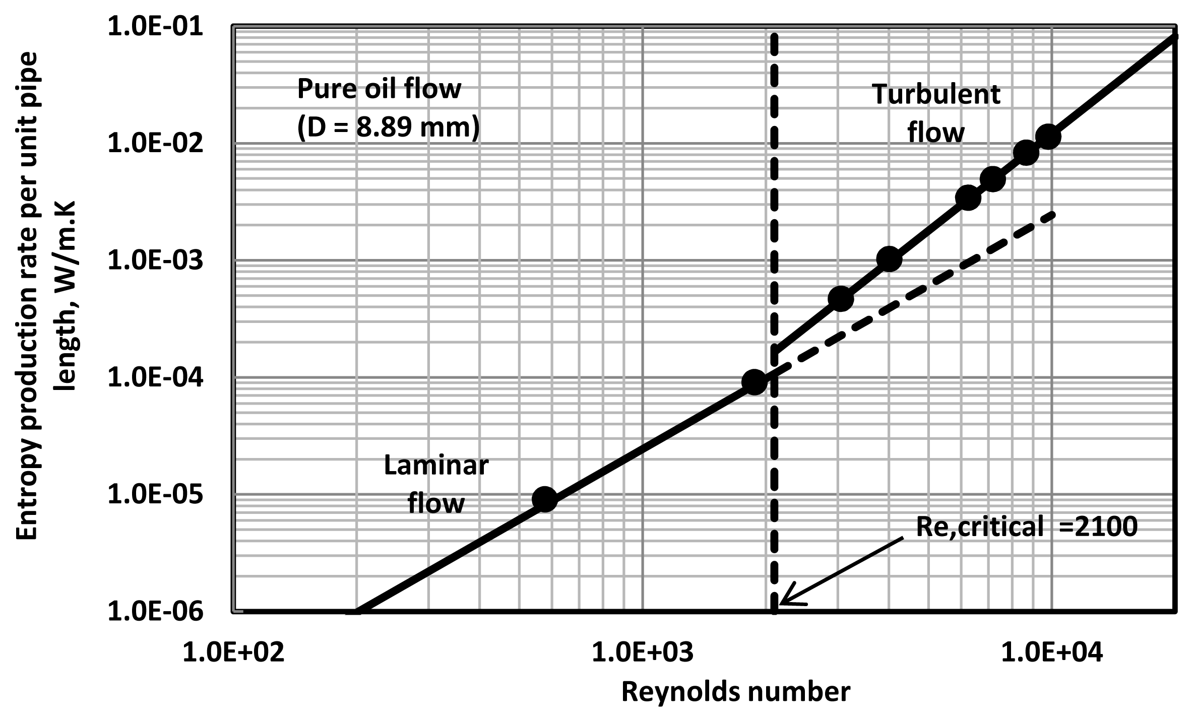
Figure 2 shows the plot of
versus Re data for pure oil flow in 8.89 mm diameter pipe. The entropy production rate
increases with the increase in Reynolds number (Re). The data (
versus Re) exhibit a linear relationship on a log-log scale in both laminar and turbulent regimes. However the slope in the turbulent regime is higher. The solid lines shown in the figure correspond to the predictions of the models, Equation (20) for laminar flow and Equation (21) for turbulent flow. The experimental data for pure oil show good agreement with the predictive models.
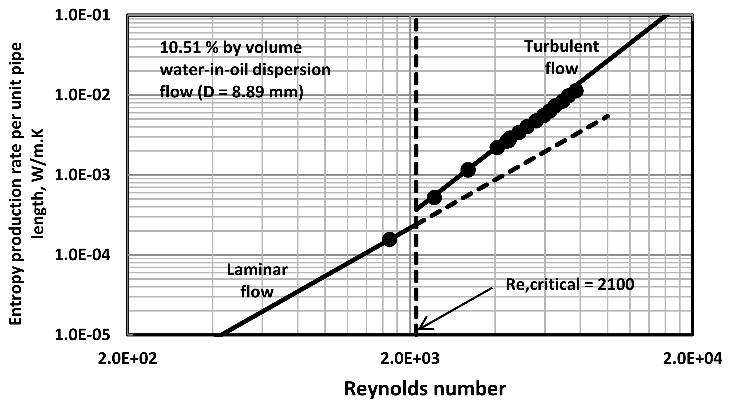
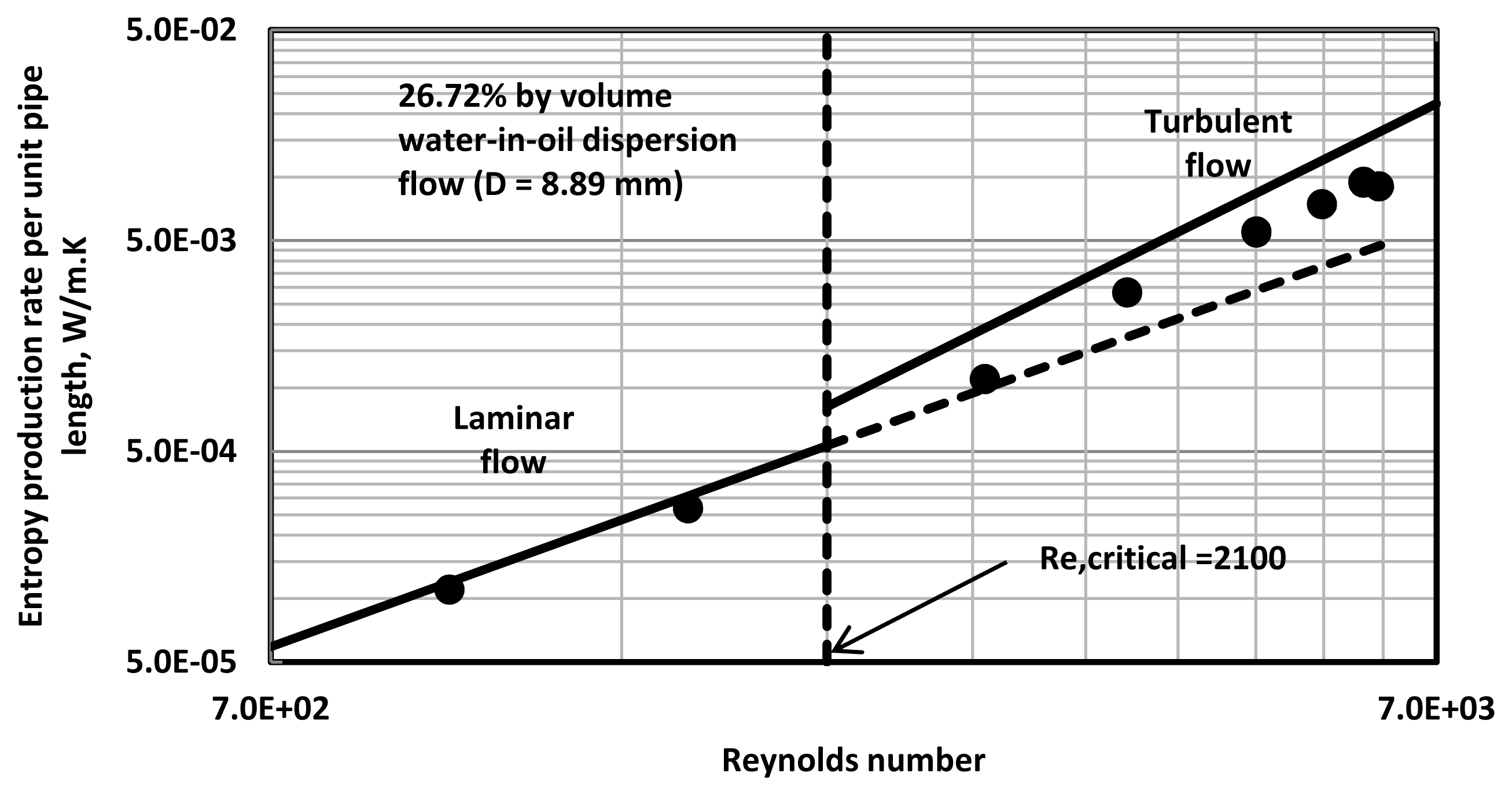
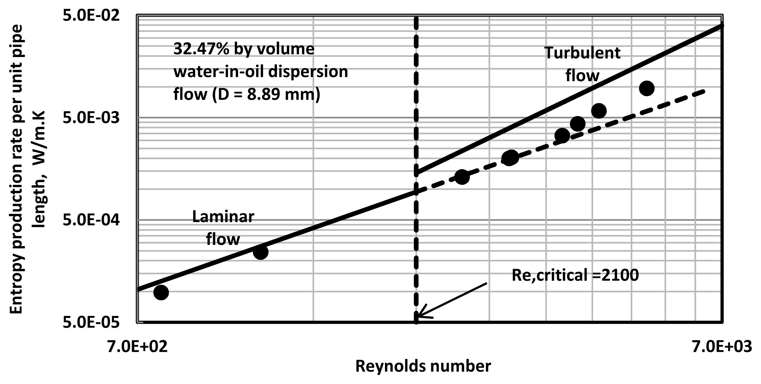
Figures 3–8 show the plots of
versus Re data for water-in-oil (W/O) emulsions with different volume fractions of the dispersed-phase (water). The pipe diameter is 8.89 mm. At low volume fractions of dispersed-phase,
versus Re data tend to follow the single-phase lines. However, at high volume fractions of the dispersed-phase, the entropy production rates in turbulent flow of emulsions are significantly lower than the values expected for single-phase fluids with the same properties (that is, Equation (21)).
The addition of water droplets to oil clearly causes suppression of turbulence resulting in lower dissipation of energy and hence lower rate of entropy production. Interestingly, critical Reynolds number where transition from laminar regime to turbulent regime occurs increases with the increase in dispersed-phase concentration.
In the case of 41.05% by volume water-in-oil emulsion, the experimental data (see Figure 8) shows complete suppression of turbulence and therefore, the entropy production rates follow the laminar flow line even though the Reynolds number is much higher than 2100, the critical value for single-phase Newtonian fluids.
Figure 9 shows the plot of the ratio of entropy production rate in emulsion flow to entropy production rate in single-phase Newtonian flow (same viscosity and density) at the same Reynolds number of approximately 4000. The ratio decreases with the increase in dispersed-phase concentration. At the dispersed-phase (water) volume fraction of 0.41, the ratio is 0.384. Thus the presence of water droplets in pipeline flow of oil is advantageous thermodynamically in that the entropy production rates are reduced significantly due to suppression of turbulence by water droplets.
The influence of pipe diameter on entropy production rates is shown in Figure 10. The plots shown in Figure 10 are generated from single-phase Equations (20) and (21) using the properties of oil. With the increase in pipe diameter at a given Reynolds number, the entropy production rate decreases. This same trend is exhibited in emulsion flow. Figures 11 and 12 show the influence of pipe diameter on entropy production rates in emulsion flow at two different dispersed-phase concentrations. The entropy production rate decreases with the increase in pipe diameter as expected in both laminar and turbulent regimes. However, the data falls well below the single phase lines in turbulent flow as already noted in the preceding discussion.
5. Conclusions
Based on the experimental work and analysis of entropy production in pipeline adiabatic flow of water-in-oil emulsions, the following conclusions can be made: (a) the entropy production rate per unit length of pipe increases with the increase in Reynolds number; (b) the entropy production rate decreases with the increase in pipe diameter at the same Reynolds number; (c) the entropy production rates in emulsion flow can be described adequately by single-phase Newtonian flow equations only in the laminar regime; (d) in the turbulent regime, the entropy production rates in emulsion flow are found to be substantially smaller than those expected on the basis of single-phase flow equations. The deviation from single-phase flow behavior increases with the increase in dispersed-phase concentration. For example, the entropy production rate in water-in-oil emulsion flow at a dispersed-phase volume fraction of 0.41 is only 38.4% of that observed in the flow of a single-phase Newtonian fluid with the same viscosity and density, when comparison is made at a Reynolds number of 4000; and (e) the deviation in entropy production rate of emulsion flow from that of single-phase fluid is due to suppression of turbulence caused by the presence of dispersed droplets.
Acknowledgment
Financial support from NSERC is appreciated.
Conflicts of Interest
The author declares no conflict of interest.
References
- Smith, J.M.; Van Ness, H.C.; Abbott, M.M. Introduction to Chemical Engineering Thermodynamics, 7th ed.; McGraw-Hill: New York, NY, USA, 2005; pp. 635–636. [Google Scholar]
- Abbott, M.M.; Van Ness, H.C. Theory and Problems of Thermodynamics, 2nd ed.; Schaum’s Outline Series; McGraw-Hill: New York, NY, USA, 1989; pp. 302–307. [Google Scholar]
- Cengel, Y.; Boles, M. Thermodynamics: An Engineering Approach, 7th ed.; McGraw-Hill: New York, NY, USA, 2011; Volume Chapter 8. [Google Scholar]
- Pal, R. Rheology of Particulate Dispersions and Composites; CRC Press: Boca Raton, FL, USA, 2007. [Google Scholar]
- Pal, R. Effect of droplet size on the rheology of emulsions. AIChE J 1996, 42, 3181–3190. [Google Scholar]
- Pal, R. Pipeline flow of unstable and surfactant-stabilized emulsions. AIChE J 1993, 39, 1754–1764. [Google Scholar]
- Hwang, C.Y.J.; Pal, R. Flow of two-phase oil/water mixtures through sudden expansions and contractions. Chem. Eng. J 1997, 68, 157–163. [Google Scholar]
- Pal, R. Rheology of simple and multiple emulsions. Curr. Opin. Colloid Interface Sci 2011, 16, 41–60. [Google Scholar]
- Pal, R. Techniques for measuring the composition (oil and water content) of emulsions—A state of the art review. Colloids Surf. A 1994, 84, 141–193. [Google Scholar]
- Ngan, K.H.; Ioannou, K.; Rhyne, L.D.; Wang, W.; Angeli, P. A methodology for predicting phase inversion during liquid-liquid dispersed pipeline flow. Chem. Eng. Res. Des 2009, 87, 318–324. [Google Scholar]
- Liu, L.; Matar, O.K.; Lawrence, C.J.; Hewitt, G.F. Laser-induced fluorescence (LIF) studies of liquid-liquid flows. Part I: Flow structures and phase inversion. Chem. Eng. Sci 2006, 61, 4007–4021. [Google Scholar]
- Brauner, N.; Ullmann, A. Modeling of phase inversion phenomenon in two-phase pipe flows. Intl. J. Multiph. Flow 2008, 28, 1177–1204. [Google Scholar]
- Piela, K.; Delfos, R.; Ooms, G.; Westerweel, J.; Oliemans, R.V.A.; Mudde, R.F. Experimental investigation of phase inversion in an oil-water flow through a horizontal pipe loop. Int. J. Multiph. Flow 2006, 32, 1087–1099. [Google Scholar]
- Piela, K.; Delfos, R.; Ooms, G.; Westerweel, J.; Oliemans, R.V.A. On the phase inversion process in an oil-water flow. Int. J. Multiph. Flow 2008, 34, 665–677. [Google Scholar]
- Xu, J.Y.; Li, D.H.; Guo, J.; Wu, Y.X. Investigations of phase inversion and frictional pressure gradient in upward and downward oil-water flow in vertical pipes. Int. J. Multiph. Flow 2010, 36, 930–939. [Google Scholar]
- Simmons, M.J.H.; Azzopardi, B.J. Drop size distribution in dispersed liquid-liquid pipe flow. Int. J. Multiph. Flow 2001, 27, 843–859. [Google Scholar]
- Angeli, P.; Hewitt, G.F. Drop size distributions in horizontal oil-water dispersed flows. Chem. Eng. Sci 2000, 55, 3133–3143. [Google Scholar]
- Wang, W.; Cheng, W.; Duan, J.; Gong, J.; Hu, B.; Angeli, P. Effect of dispersed holdup on drop size distribution in oil-water dispersions: Experimental observations and population balance modeling. Chem. Eng. Sci 2014, 105, 22–31. [Google Scholar]
- Liao, Y.; Lucas, D. A literature review of theoretical models for drop and bubble breakup in turbulent dispersions. Chem. Eng. Sci 2009, 64, 3389–3406. [Google Scholar]
- Jana, A.K.; Das, G.; Das, P.K. Flow regime identification of two-phase liquid-liquid upflow through vertical pipe. Chem. Eng. Sci 2006, 61, 1500–1515. [Google Scholar]
- Angeli, P.; Hewitt, G.F. Flow structure in horizontal oil-water flow. Int. J. Multiph. Flow 2000, 26, 1117–1140. [Google Scholar]
- Lum, J.Y.L.; Al-Wahaibi, T.; Angeli, P. Upward and downward inclination oil-water flows. Int. J. Multiph. Flow 2006, 32, 413–435. [Google Scholar]
- Lovick, J.; Angeli, P. Experimental studies on the dual continuous flow pattern in oil-water flows. Int. J. Multiph. Flow 2004, 30, 139–157. [Google Scholar]
- Lu, Y.; He, L.; He, Z.; Wang, A. A study of pressure gradient characteristics of oil-water dispersed flow in horizontal pipe. Energy Procedia 2012, 16, 1111–1117. [Google Scholar]
- Al-Wahaibi, T. Pressure gradient correlation for oil-water separated flow in horizontal pipes. Exp. Therm. Fluid Sci 2012, 42, 196–203. [Google Scholar]
- Angeli, P.; Hewitt, G.F. Pressure gradient in horizontal liquid-liquid flows. Int. J. Multiph. Flow 1998, 24, 1183–1203. [Google Scholar]
- Bejan, A. Entropy Generation through Heat and Fluid Flow; Wiley & Sons: New York, NY, USA, 1982; pp. 105–107. [Google Scholar]
Figure 1.
Schematic diagram of the flow rig.

Figure 2.
versus Re plot for pure oil flow in a 8.89 mm diameter pipeline.

Figure 3.
versus Re plot for 10.51% by vol. W/O emulsion flow in a 8.89 mm diameter pipeline.

Figure 4.
versus Re plot for 17.49% by vol. W/O emulsion flow in a 8.89 mm diameter pipeline.

Figure 5.
versus Re plot for 26.72% by vol. W/O emulsion flow in a 8.89 mm diameter pipeline.

Figure 6.
versus Re plot for 32.47% by vol. W/O emulsion flow in a 8.89 mm diameter pipeline.

Figure 7.
versus Re plot for 38.14% by vol. W/O emulsion flow in a 8.89 mm diameter pipeline.

Figure 8.
versus Re plot for 41.05% by vol. W/O emulsion flow in a 8.89 mm diameter pipeline.

Figure 9.
Influence of dispersed-phase volume fraction of emulsion on the ratio of entropy production rate in emulsion flow to entropy production rate in single-phase Newtonian flow with the same properties (viscosity and density).
Figure 9.
Influence of dispersed-phase volume fraction of emulsion on the ratio of entropy production rate in emulsion flow to entropy production rate in single-phase Newtonian flow with the same properties (viscosity and density).

Figure 10.
Influence of pipe diameter on entropy production rate in single-phase Newtonian flow.

Figure 11.
Influence of pipe diameter on entropy production rate in 38.14% by vol. W/O emulsion flow.
Figure 11.
Influence of pipe diameter on entropy production rate in 38.14% by vol. W/O emulsion flow.

Figure 12.
Influence of pipe diameter on entropy production rate in 41.05% by vol. W/O emulsion flow.
Figure 12.
Influence of pipe diameter on entropy production rate in 41.05% by vol. W/O emulsion flow.


| Pipe inside diameter (mm) | Entrance length (m) | Length of test section (m) | Exit length (m) |
|---|---|---|---|
| 8.89 | 0.89 | 3.35 | 0.48 |
| 12.60 | 1.19 | 2.74 | 0.53 |
| 15.8 | 1.65 | 2.59 | 0.56 |
© 2014 by the authors; licensee MDPI, Basel, Switzerland This article is an open access article distributed under the terms and conditions of the Creative Commons Attribution license (http://creativecommons.org/licenses/by/3.0/).
Share and Cite
MDPI and ACS Style
Pal, R. Entropy Production in Pipeline Flow of Dispersions of Water in Oil. Entropy 2014, 16, 4648-4661. https://doi.org/10.3390/e16084648
AMA Style
Pal R. Entropy Production in Pipeline Flow of Dispersions of Water in Oil. Entropy. 2014; 16(8):4648-4661. https://doi.org/10.3390/e16084648
Chicago/Turabian StylePal, Rajinder. 2014. "Entropy Production in Pipeline Flow of Dispersions of Water in Oil" Entropy 16, no. 8: 4648-4661. https://doi.org/10.3390/e16084648