Information Anatomy of Stochastic Equilibria

Abstract

A stochastic nonlinear dynamical system generates information, as measured by its entropy rate. Some—the ephemeral information—is dissipated and some—the bound information—is actively stored and so affects future behavior. We derive analytic expressions for the ephemeral and bound information in the limit of infinitesimal time discretization for two classical systems that exhibit dynamical equilibria: first-order Langevin equations (i) where the drift is the gradient of an analytic potential function and the diffusion matrix is invertible and (ii) with a linear drift term (Ornstein–Uhlenbeck), but a noninvertible diffusion matrix. In both cases, the bound information is sensitive to the drift and diffusion, while the ephemeral information is sensitive only to the diffusion matrix and not to the drift. Notably, this information anatomy changes discontinuously as any of the diffusion coefficients vanishes, indicating that it is very sensitive to the noise structure. We then calculate the information anatomy of the stochastic cusp catastrophe and of particles diffusing in a heat bath in the overdamped limit, both examples of stochastic gradient descent on a potential landscape. Finally, we use our methods to calculate and compare approximations for the time-local predictive information for adaptive agents.

1. Introduction

If we track the position of a particle diffusing on an unchanging potential long enough, we can estimate the probability of observing a sequence of positions [1]. From that, we can quantitatively answer questions about the process’s behavior using a range of information statistics that answer specific questions:

• How random is it? The entropy rate h_μ, which is the entropy in the present observation conditioned on all past observations [2].
• What must be remembered about the past in order to optimally predict the future? The causal states, which are groupings of pasts that lead to the same probability distribution over future trajectories [3,4].
• How much memory is required to store these causal states? The statistical complexity C_μ, or the entropy of the causal states [3].
• How much of the future is predictable from the past? The excess entropy E, which is the mutual information between the past and the future [5].
• How much of the generated information (h_μ) is relevant to predicting the future? The bound information b_μ, which is the mutual information between the present and future observations conditioned on all past observations [6].
• How much of the generated information is useless (neither affects future behavior nor contains information about the past)? The ephemeral information r_μ, which is the entropy in the present observation conditioned on all past and future observations [6].

These informational quantities usually cannot be deduced from a bifurcation diagram, so we see them as providing a complementary view of a process’s structure and behavior.

In applications, such informational characterizations of a time series are useful for monitoring good sensory coding [7], cognitive modalities [8], brain coherence [9], hidden Markov model structural inference [10], action policies of autonomous agents [11,12], structure in disordered materials [13,14], dynamical phase transitions [15,16] and intrinsic information processing in deterministic chaos [17,18] and cellular automata [19,20].

Here, we focus on continuous stochastic nonlinear dynamical systems, the theory for which has a long and venerable history, has met with a number of successful predictions, and has identified a number of principles describing how noise interacts with nonlinearity [21]. For nonlinear systems transitioning to chaos, to take just one example, noise plays the role of a “disordering” field, just as the magnetic field is an ordering field for spin systems at critical transitions [22,23]. Though their history substantially predates that of the wide range of complex systems applications just cited, relatively fewer analyses of their information processing components—their information anatomy—have been carried out. As a start, we demonstrate how to calculate the quantities above for continuous-time, continuous-state stochastic nonlinear systems exhibiting dynamical equilibria, yielding intuition for the properties these measures capture in simpler, and perhaps more familiar, physical models.

Throughout, we focus on a ubiquitous and simple nonlinear generative model: stochastic gradient descent or, in other words, diffusion on a potential surface. We assume infinite precision in our observation of the state space. The first calculation assumes that the diffusion matrix is invertible and drift is analytic; the second assumes that the drift term is linear, but allows for a noninvertible diffusion matrix. All calculations assume that the time between measurements is nonzero, but arbitrarily small, and that all derived information anatomy quantities are finite at finite temporal coarse-graining.

There are alternative ways to frame information analyses of continuous stochastic processes [24]. The one we take is rather prosaic, paralleling the “physics” approach laid out by Gaspard and Wang [25], who coarse-grain time at a finite, but small, time scale τ and state-space at a similar spatial scale ε. This discretizes the calculations and then one takes the limits τ → 0 and ε → 0. Crucially, the limits often reveal divergences in the informational quantities. For example, it is well known that the (ε, τ )-entropy of a broad family of continuous stochastic processes diverges [25]. However, as Gaspard and Wang demonstrate and as is familiar in other fundamental physics domains, the form of the divergences captures important structural properties. The main deviation here from their approach is that we employ the Shannon differential entropy to side-step state-space (ε) coarse-graining.

An alternative, and insightful, framing considers the divergences to be unnatural; in particular, with naive coarse-graining, it is difficult to establish ergodic theorems key to information theory. In this view, the main concern translates into a search for tractable definitions of information measures that finitely quantify information processing in continuous stochastic systems. To address divergences, one investigates a given stochastic process relative to Brownian motion. In a crude sense, the known Brownian base case carries the divergences. To factor them out of the given process, one employs Girsanov’s theorem to transform the given process to a canonical Brownian motion with the same diffusion [26]. Properties of the transformation then characterize the given process’s informational properties; for example, giving a relative entropy rate. This strikes us as an important avenue for future investigation; one that, to be clear, is not yet completed, as far as we know, and one that eventually will be related to the more prosaic, physics framing that we address here.

To get started, background is given in Section 2. Results are presented in Section 3 and stated more succinctly in

Table 1. Information anatomy of first-order, n-dimensional nonlinear Langevin dynamics: ẋ = −D∇U(x) + η(t), where U(x) is analytic in x and η(t) is zero-mean white noise with invertible diffusion matrix D, 〈η(t)η(t′)^⊤ 〉 = Dδ(t − t′). Stationary distribution ρ_eq(x) ∝ exp(−2U(x)) is assumed normalizable.

Information Rates	Definition	Terms
		O(τ−1 log τ)	O(τ−1)	O(1)
Stored H0 = Cμ(τ)	$\frac{H[X_0]}{\tau }$	0	−∫ ρeq(x) log ρeq(x)dx	0
τ-Entropy hμ(τ)	$\frac{H[X_0\mid X_{:0}]}{\tau }$	$\frac{n}{2}$	$\text{log\hspace{0.17em}}\sqrt{2\pi e\mid \text{det\hspace{0.17em}}D\mid }+n\hspace{0.17em}\text{log\hspace{0.17em}}\sqrt{2}$	$-\frac{1}{2}\int \nabla ·(D\nabla U(x)){\rho }_{eq}(x)dx$
Bound bμ(τ)	$\frac{I[X_0;X_{\tau :}\mid X_{:0}]}{\tau }$	0	$n\hspace{0.17em}\text{log\hspace{0.17em}}\sqrt{2}$	$-\frac{1}{2}\int \nabla ·(D\nabla U(x)){\rho }_{eq}(x)dx$
Ephemeral rμ(τ)	$\frac{H[X_0\mid X_{:0},X_{\tau :}]}{\tau }$	$\frac{n}{2}$	$\text{log\hspace{0.17em}}\sqrt{2\pi e\mid \text{det\hspace{0.17em}}D\mid }$	0
Enigmatic qμ(τ)	$\frac{I[X_{:0};X_0;X_{\tau :}]}{\tau }$	$-\frac{n}{2}$	$-\int {\rho }_{eq}(x)\hspace{0.17em}\text{log\hspace{0.17em}}{\rho }_{eq}(x)dx-n\hspace{0.17em}\text{log\hspace{0.17em}}2-\text{log\hspace{0.17em}}\sqrt{2\pi e\mid \text{det\hspace{0.17em}}D\mid }$	∫ ∇ · (D∇U(x))ρeq(x)dx
Elusive σμ(τ)	$\frac{I[X_{:0};X_{\tau :}\mid X_0]}{\tau }$	0	0	0

. To illustrate how to apply those formulae, we calculate the information anatomy of the stochastic cusp catastrophe in Section 4.1 and of coupled particles diffusing in a heat bath in Section 4.2.

We provide a suite of appendices that are home to technical details necessary for completeness, but that would otherwise distract. Several appendices also draw out implications of information anatomy analysis. Appendix A shows that the information anatomy of a Markov system requires looking only one time step into the future and past, as expected from a similar calculation in [6]. Appendix B establishes that the causal states of a first-order Langevin equation with an analytic drift are isomorphic to the present position. Appendix C justifies why, given an infinitesimal time resolution τ, the conditional entropy of the measurement at a future time step given the present measurement can be approximated arbitrarily well by using a linearized drift term when the diffusion matrix is invertible. Appendix D then demonstrates that the entropy of the Green’s function of a linear Langevin equation with a noninvertible diffusion matrix differs from that when the diffusion matrix is invertible. Finally, Appendix E applies the formulae in Appendices A–C to explore estimates of the time-local predictive information and related alternatives, used as optimization principles to choose action policies for adaptive autonomous agents [12].

2. Background

Let us first recall the information anatomy analysis of discrete-time, discrete-state processes introduced in [6]. The main object of study is a process ℘: the list of all of a system’s behaviors or realizations {… x₋₂, x₋₁, x₀, x₁, …} and their probabilities, specified by the joint distribution Pr(…X₋₂, X₋₁, X₀, X₁, …). We denote a contiguous chain of random variables as X_0:L = X₀X₁ · · ·X_L−1. We assume the process is ergodic and stationary (Pr(X_0:L) = Pr(X_t:L+t) for all t ∈ ℤ) and the measurement symbols range over a finite alphabet: x ∈ . In this setting, the present X₀ is the random variable measured at t = 0, the past is the chain X_:0 = …X₋₂X₋₁ leading up the present and the future is the chain following the present X_1: = X₁X₂ · · ·. (We suppress the infinite index in these.)

Shannon’s various information quantities—entropy, conditional entropy, mutual information, and the like—when applied to time series are functions of the joint distributions Pr(X_0:L). Importantly, they define an algebra of information measures for a given set of random variables [27]. James et al. [6] used this to show that the past and future partition the single-measurement entropy H(X₀) into several measure-theoretic atoms. These include the ephemeral information:

$$r_{\mu }=H[X_0\mid X_{:0},X_{1:}],$$

which measures the uncertainty of the present knowing the past and future; the bound information:

$$b_{\mu }=I[X_0;X_{1:}\mid X_{:0}],$$

which is the information shared between present, and future conditioned on past; and the enigmatic information:

$$q_{\mu }=I[X_0;X_{:0};X_{1:}],$$

which is the co-information between past, present and future.

For a stationary time series, the bound information is also the shared information between present and past conditioned on the future:

$$b_{\mu }=I[X_0;X_{:0}\mid X_{1:}].$$

One can also consider the amount of predictable information not captured by the present:

$${\sigma }_{\mu }=I[X_{:0};X_{1:}\mid X_0].$$

which is called the elusive information. It measures the amount of past-future correlation not contained in the present. It is nonzero if the process has “hidden states” and is therefore quite sensitive to how the state space is “observed” or coarse-grained.

The total information in the future predictable from the past (or vice versa) is the excess entropy:

$$\mathbf{E}=I[X_{:1};X_{1:}]=b_{\mu }+{\sigma }_{\mu }+q_{\mu }.$$

The process’s Shannon entropy rate h_μ can also be written as a sum of atoms:

$$h_{\mu }=H[X_0\mid X_{:0}]=r_{\mu }+b_{\mu }.$$

Thus, a portion of the information (h_μ) a process spontaneously generates is thrown away (r_μ) and a portion is actively stored (b_μ). Putting these observations together gives the information anatomy of a single measurement:

$$H[X_0]=q_{\mu }+2b_{\mu }+r_{\mu }.$$

(1)

These quantities were originally defined for stationary processes, but easily carry over to a nonstationary process of finite Markov order. (See Appendix A.)

The burden of the following is to analyze the limit from the discrete-time, discrete-value processes just discussed to continuous-time, continuous-value processes. Suppose that observations are made at very small intervals of duration τ. Then, the observation at time t_n = nτ is now labeled X_nτ, and the past X_:0 is now denoted …X_−2τX_−τ instead of …X₋₂X₋₁. Rather than entropy or mutual information per observed symbol, as in the discrete time setting, we define an entropy or mutual information per elapsed time unit; that is, informational rates. A step in this direction is to normalize the information measures defined above by the observation interval:

$$\begin{array}{l}{r}_{\mu }(\tau )=H[X_0\mid X_{:0},X_{\tau :}]/\tau ,\\ b_{\mu }(\tau )=I[X_{\tau :};X_0\mid X_{:0}]/\tau ,\\ q_{\mu }(\tau )=I[X_{:0};X_0;\mid X_{\tau :}]/\tau ,\\ {\sigma }_{\mu }(\tau )=I[X_{:0};X_{\tau :}\mid X_0]/\tau ,\end{array}$$

and

$$H_0(\tau )=H[X_0]/\tau .$$

We normalize the entropy H[X₀] of a single symbol by the time resolution τ to preserve the form of the information-theoretic relationship given in Equation (1). In doing so, we no longer interpret H₀(τ ) as the entropy of a single measurement symbol, but rather as the number of bits per unit time required to encode the time series in a model-free manner.

In contrast with the original information anatomy interpretation given in [6], we think of h_μ(τ) as the minimal achievable coding rate, were we to build a maximally predictive model. In this time normalization, terms of order τ or higher are ignored. These definitions then lead to the τ-entropy rate familiar in the discrete-time, continuous-value setting [2,25,28]:

$$h_{\mu }(\tau )=H[X_0\mid X_{:0}]/\tau .$$

More natural definitions of these quantities might involve a fully continuous-time development that avoids the log τ divergences of the τ entropy rate [29]. As noted in the Introduction, however, we leave alternative developments for the future. When considering continuous-value processes, we use the differential entropy, thereby regularizing away the log ε divergences seen in the (ε, τ )-entropy rate [25].

Figures 1(a) and 1(b) give information diagrams that illustrate the algebra of the information measure atoms just defined. There, the entropy of a set is the sum of the entropy of its atoms. This reveals several useful linear dependencies that were originally noted in [6]:

$$\begin{array}{l}{H}_0(\tau )=r_{\mu }(\tau )+2b_{\mu }(\tau )+q_{\mu }(\tau ),\\ h_{\mu }(\tau )=r_{\mu }(\tau )+b_{\mu }(\tau ),\end{array}$$

and

$$\mathbf{E}/\tau =q_{\mu }(\tau )+{\sigma }_{\mu }(\tau )+b_{\mu }(\tau ).$$

For a Markov process, illustrated in Figure 1b, the elusive information vanishes:

$${\sigma }_{\mu }(\tau )=0.$$

Therefore, in this case, if we find expressions for H₀(τ), h_μ(τ) and b_μ(τ), then we can find r_μ(τ), q_μ(τ) and E/τ via:

$$q_{\mu }(\tau )=H_0(\tau )-h_{\mu }(\tau )-b_{\mu }(\tau ),$$

(2)

$$r_{\mu }(\tau )=h_{\mu }(\tau )-b_{\mu }(\tau ),$$

(3)

and

$$\mathbf{E}/\tau =H_0(\tau )-h_{\mu }(\tau ).$$

(4)

3. Information Anatomy of Stochastic Dynamical Systems

To determine a process’s information anatomy, one must calculate entropies and conditional entropies of the joint probability distribution of the entire past, the present, and the entire future. In the general case, this is challenging. However, since the first-order Langevin equations we consider are Markov, we have:

$$\tau h_{\mu }(\tau )=H[X_{\tau }\mid X_0]$$

(5)

and

$$\tau b_{\mu }(\tau )=H[X_{\tau };X_{-\tau }]-H[X_{\tau };X_0].$$

(6)

(Appendix A provides the derivation.) Therefore, to calculate a Markov process’s information anatomy, we need only the joint probability distribution of three successive measurements instead of the joint probability distribution of the present and semi-infinite past and future. To further simplify the calculation of conditional entropies, we assume that τ is small enough that the entropy of the Green’s function—i.e., the transition probabilities P(x′, t + τ |x, t)—is well approximated by the entropy of a corresponding Gaussian. This is exactly true for a linear Langevin equation. For a nonlinear Langevin equation, the Gaussian approximation is valid in the limit of infinitesimal τ. (Appendix C calculates small-τ approximations for the variance of this Gaussian.) We do not approximate the stationary distribution of a nonlinear Langevin equation by a Gaussian, however, and this means that the joint probability distribution over successive measurements is in general highly non-Gaussian. Finally, we assume that all derived information anatomy quantities are finite (at finite τ) and that there is a normalizable stationary probability distribution.

Appendix B shows that, for first-order Langevin dynamics, the single-measurement entropy H[X₀] is the process’s statistical complexity C_μ [3,4]. The result is that the information anatomy analysis decomposes this causal-state information into:

• that useful for prediction or retrodiction beyond the information provided by the causal states at the previous time step—the bound information b_μ;
• that useful for both prediction and retrodiction—the co-information q_μ; and
• that useless for both prediction and retrodiction—the ephemeral information rate r_μ.

This is a similar, but finer C_μ decomposition than considered in [30]. There, and more generally, C_μ = E + χ. That is, the state information consists of that shared with the future (E) and information not shared with the future, but that must be stored to implement optimal prediction—the crypticity χ [31]. Together with these observations, Equation (4) reminds us that χ = h_μ for Markov processes, as originally noted for finite-range one-dimensional spin systems [32].

3.1. Nonlinear Langevin Dynamics

Consider an n-dimensional nonlinear Langevin equation:

$$\frac{dx}{dt}=-D\nabla U(x)+\eta (t),$$

where x ∈ ℝⁿ, U(x) is an analytic potential function and η(t) is zero-mean white noise with diffusion matrix D: 〈η_i(t)〉 = 0 and 〈η_i(t)η_j(t′)〉 = D_ijδ(t−t′). The diffusion coefficients D_ij = D_ji are assumed to be independent of x and such that det D ≠ 0. The following (well known) stationary distribution is derived by converting the stochastic differential equation into its Fokker–Planck equation form:

$${\rho }_{eq}(x)=\frac{1}{Z}\text{exp\hspace{0.17em}}(-2U(x)),$$

(7)

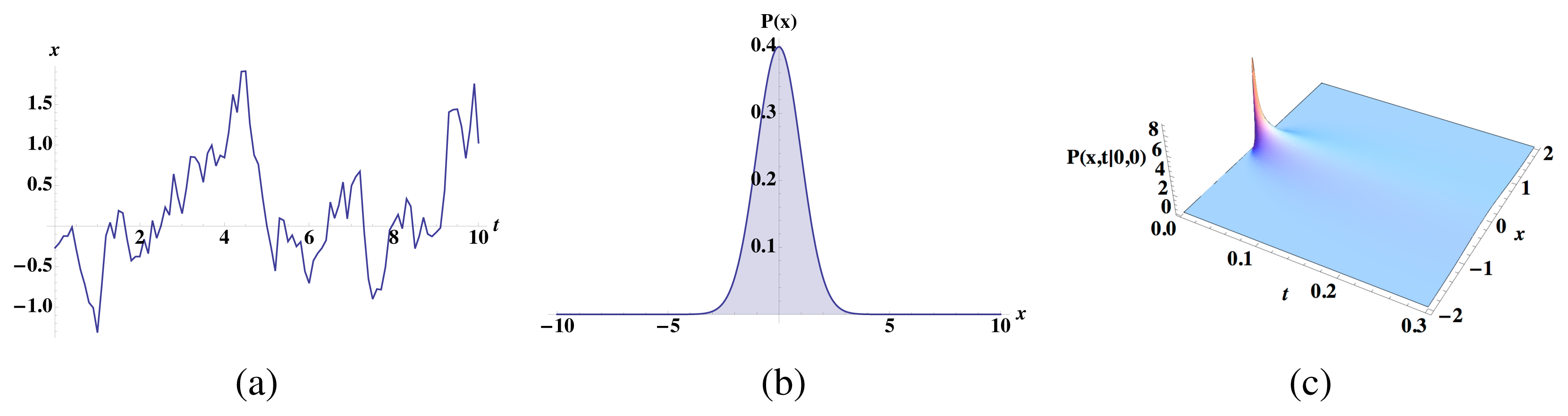
where Z = ∫ e^−2U(x)dx. We assume that this is the stationary probability distribution experienced by the particle and that it is normalizable: Z < ∞. (See Figure 2 for simulation results in one dimension.)

The time-discretization normalized entropy of a measurement is:

$$H_0=-\frac{1}{\tau }\int {\rho }_{eq}(x)\hspace{0.17em}\text{log\hspace{0.17em}}{\rho }_{eq}(x)dx.$$

(8)

The conditional entropies H[X_τ |X₀] and H[X_τ |X_−τ] in Equations (5) and (6) can be calculated, simplifying if the conditional probabilities Pr(X_τ |X₀) and Pr(X_τ |X_−τ) are Gaussians, using:

$$H[X_{\tau }\mid X_0]=\int {\rho }_{eq}(x^{\prime })H[X_{\tau }\mid X_0=x^{\prime }]d{x}^{\prime }$$

and

$$H[X_{\tau }\mid X_{-\tau }]=\int {\rho }_{eq}(x^{\prime })H[X_{\tau }\mid X_{-\tau }=x^{\prime }]d{x}^{\prime }.$$

This yields:

$$H[X_{\tau }\mid X_0=x^{\prime }]=\frac{1}{2}\text{log\hspace{0.17em}}(2\pi e\mid \text{det\hspace{0.17em}Var}{(X_{\tau })}_{p(X_{\tau }\mid X_0=x^{\prime })}\mid )$$

(9)

and

$$H[X_{\tau }\mid X_{-\tau }=x^{\prime }]=\frac{1}{2}\text{log\hspace{0.17em}}(2\pi e\mid \text{det\hspace{0.17em}Var}{(X_{\tau })}_{p(X_{\tau }\mid X_{-\tau }=x^{\prime })}\mid ).$$

(10)

Appendix C gives a plausibility proof that the conditional distributions Pr(X_τ |X₀) and Pr(X_τ |X_−τ ) are Gaussian to o(τ) over a region of ℝⁿ with measure arbitrarily close to one. The entropies of these Gaussians are calculable to leading and subleading order in τ using a linearized version of the nonlinear Langevin equation about the initial position:

$$\frac{dx}{dt}=\nabla U(x){\mid }_{x=x^{\prime }}+A(x^{\prime })\hspace{0.17em}(x-x^{\prime })+\eta (t)+O({\Vert x-x^{\prime }\Vert }^2).$$

where A(x′) is a matrix with entries (A(x′))_ij = ∂(D∇U)_j/∂x_i. (This is similar, but not identical to the approximation used in [12]. Appendix E comments on the differences.) From Appendix C, we have that:

$$\text{Var}{(X_{\tau })}_{p(X_{\tau }\mid X_0=x^{\prime })}=D\tau +\frac{\nabla \mu (x)D+D{(\nabla \mu (x))}^{\top }}{2}{\tau }^2+O({\tau }^3)$$

(11)

and, similarly,

$$\text{Var}{(X_{\tau })}_{p(X_{\tau }\mid X_{-\tau }=x^{\prime })}=2D\tau +2(\nabla \mu (x)D+D{(\nabla \mu (x))}^{\top }){\tau }^2+O({\tau }^3).$$

(12)

Substituting Equations (11) and (12) into Equations (9) and (10), respectively, gives, with some algebra:

$$H[X_{\tau }\mid X_{-\tau }]=-\tau \int {\rho }_{eq}(x)\nabla ·(D\nabla U(x))dx+\text{log\hspace{0.17em}}\sqrt{2^{n+1}\pi e\mid \text{det\hspace{0.17em}}D\mid {\tau }^n}$$

(13)

and:

$$H[X_{\tau }\mid X_0]=-\frac{\tau }{2}\int {\rho }_{eq}(x)\nabla ·(D\nabla U(x))dx+\text{log\hspace{0.17em}}\sqrt{2\pi e\mid \text{det\hspace{0.17em}}D\mid {\tau }^n}.$$

(14)

Substituting Equation (14) into Equation (5), we find that:

$$h_{\mu }(\tau )=\frac{n\hspace{0.17em}\text{log\hspace{0.17em}}\sqrt{2\tau }}{\tau }+\frac{\text{log\hspace{0.17em}}\sqrt{\pi e\mid \text{det\hspace{0.17em}}D\mid }}{\tau }-\frac{1}{2}\int {\rho }_{eq}(x)\nabla ·(D\nabla U)dx+o(1).$$

(15)

The leading order term is recognizable as an (ε, τ)-entropy rate of the Ornstein–Uhlenbeck process [25], except that the ε has been regularized away, since we used Shannon’s differential entropy. Substituting Equations (13) and (14) into Equation (6), we find the bound information rate:

$$b_{\mu }(\tau )=\frac{n\hspace{0.17em}\text{log\hspace{0.17em}}\sqrt{2}}{\tau }-\frac{1}{2}\int {\rho }_{eq}(x)\nabla ·(D\nabla U(d))dx+o(1).$$

(16)

Thus, the rate of active information storage depends on the dimension of the state space to leading order in τ, but its nondivergent part depends on the average curvature of the potential.

From these quantities, all other anatomy measures follow. Substituting Equations (15) and (16) into Equation (3), we find that the ephemeral information is:

$$r_{\mu }(\tau )=\frac{n\hspace{0.17em}\text{log\hspace{0.17em}}\sqrt{\tau }}{\tau }+\frac{\text{log\hspace{0.17em}}\sqrt{2\pi e\mid \text{det\hspace{0.17em}}D\mid }}{\tau }+o(1).$$

(17)

Unsurprisingly, the dissipated information—that entropy created in the present useful for neither predicting nor retrodicting—depends only on the noisiness of the dynamics and not on the drift.

Finally, the enigmatic information—that shared between past, future, and present—follows by substituting Equations (8)–(16) into Equation (2):

$$q_{\mu }(\tau )=-\frac{1}{\tau }\int {\rho }_{eq}(x)\hspace{0.17em}\text{log\hspace{0.17em}}{\rho }_{eq}(x)dx-\frac{n\hspace{0.17em}\text{log\hspace{0.17em}}(2\sqrt{\tau })}{\tau }-\frac{\text{log\hspace{0.17em}}\sqrt{\pi e\mid \text{det\hspace{0.17em}}D\mid }}{\tau }-\int {\rho }_{eq}(x)\nabla ·(D\nabla U)dx+O(\tau ).$$

It is interesting to consider how q_μ changes as the stochasticity of the system increases: the stationary distribution ρ_eq(x) flattens out, leading to an unbounded increase in H₀. This is counteracted by an unbounded increase in the entropy rate.

We can also bound the bound information rate when ∇U grows more slowly than e^−2U with ||x||. Then, integration by parts applied to Equation (16) gives:

$$b_{\mu }(\tau )=\frac{n\hspace{0.17em}\text{log\hspace{0.17em}}\sqrt{2}}{\tau }-\frac{1}{2}\int {(\nabla U)}^{\top }D(\nabla U)\hspace{0.17em}{\rho }_{eq}(x)dx.$$

When D is positive semidefinite, with D = v^⊤ v for some vector v, then:

$$b_{\mu }(\tau )\le \frac{n\hspace{0.17em}\text{log\hspace{0.17em}}\sqrt{2}}{\tau }.$$

Therefore, b_μ(τ) is maximized when the potential well is as flat as possible, while maintaining Z < ∞.

3.2. Linear Langevin Equation with Noninvertible Diffusion

What if the invertibility of the diffusion matrix is relaxed? In particular, do we still have qualitatively the same information anatomy if a subsystem of the stochastic dynamical system evolves deterministically? How does this affect the information generation and storage properties? To this end, suppose $x={(\begin{array}{cc}{x}_d& x_n\end{array})}^{\top }$ with x ∈ ℝ^k and m = dim(x_d), where x_d evolves deterministically and x_n stochastically:

$$\frac{d{x}_d}{dt}=A_d+B_{dd}{x}_d+B_{dn}{x}_n$$

(18)

$$\frac{d{x}_n}{dt}=A_n+B_{nd}{x}_d+B_{nn}{x}_n+\eta (t).$$

(19)

Again, η(t) is white noise with 〈η(t)〉 = 0 and 〈η(t)η(t′)^⊤ 〉 = Dδ(t − t′), where D is invertible. Taken together, though, this is a linear Langevin equation for x with a noninvertible diffusion matrix. Naively assuming that the deterministic subsystem evolves with a small amount of noise, Equation (16) would apply and give, for example, to O(τ):

$$b_{\mu }=\frac{(n+m)\hspace{0.17em}\text{log\hspace{0.17em}}2}{2\tau }+\frac{\text{tr}(B_{dd})+\text{tr}(B_{nn})}{2}.$$

However, this assumption is incorrect; the noiseless limit is singular.

Since Equations (18) and (19) specify a linear Langevin equation for x, its Green’s function is Gaussian. For simplicity’s sake, we assume that $B_{dn}{D}_{nn}{B}_{dn}^{\top }$ is invertible, though it is certainly possible to derive more complicated expressions for information anatomy quantities if this does not hold. From Appendix D, to O(τ) the entropy rate is:

$$h_{\mu }(\tau )=\frac{(n+3m)\hspace{0.17em}\text{log\hspace{0.17em}}\tau }{2\tau }-\frac{m\hspace{0.17em}\text{log\hspace{0.17em}}\sqrt{12}}{\tau }+\frac{\text{log\hspace{0.17em}}\sqrt{2\pi e\mid \text{det\hspace{0.17em}}{D}_{nn}\Vert \text{det\hspace{0.17em}}{B}_{dn}{D}_{nn}{B}_{dn}^{\top }\mid }}{\tau }+\frac{\text{tr}(B_{dd})+\text{tr}(B_{nn})}{2}$$

and the bound information is:

$$b_{\mu }(\tau )=\frac{(n+3m)\hspace{0.17em}\text{log\hspace{0.17em}}2}{2\tau }+\frac{\text{tr}(B_{dd})+\text{tr}(B_{nn})}{2}.$$

(20)

Applying Equation (3), the ephemeral information rate is to O(τ):

$$r_{\mu }(\tau )=\frac{n+3m}{2}\frac{\text{log}(\tau /2)}{\tau }-\frac{m\hspace{0.17em}\text{log\hspace{0.17em}}\sqrt{12}}{\tau }+\frac{\text{log\hspace{0.17em}}\sqrt{2\pi e\mid \text{det\hspace{0.17em}}{D}_{nn}\Vert \text{det\hspace{0.17em}}{B}_{dn}{D}_{nn}{B}_{dn}^{\top }\mid }}{\tau }.$$

(21)

These answers are very different from those derived assuming that x’s deterministic subsystem x_d evolves with an infinitesimal amount of noise. The bound information in Equation (20) differs from that found from naive application of Equation (16), because the pre-factor for the log 2/τ divergence is (n + m)/2+m rather than (n+m)/2. That is, the difference counts the dimension m of the deterministically evolving state space x_d. Thus, the deterministic subsystem allows for the active storage of more of the spontaneously generated stochasticity.

The ephemeral information in Equation (21) differs from a naive application of Equation (17) in two new ways. First, the expression in Equation (21) has an additional O(1/τ) factor that is linearly proportional to the dimension m of the deterministic subsystem. Second, the term $\text{log}(2\pi e\mid \text{det\hspace{0.17em}}{D}_{nn}\Vert \text{det\hspace{0.17em}}{B}_{dn}{D}_{nn}{B}_{dn}^{\top }\mid )$ can be interpreted by supposing that $B_{dn}{D}_{nn}{B}_{dn}^{\top }$ is the effective diffusion matrix felt by the deterministically evolving states.

These information anatomy quantities are therefore sensitive to the process’s underlying noise architecture.

4. Examples

To illustrate how the information measures are helpful and interesting summaries of nonlinear Langevin dynamics, let us consider several examples.

4.1. Stochastic Gradient Descent in One Dimension

Consider a first-order nonlinear Langevin dynamics for x ∈ ℝ in which:

$$\frac{dx}{dt}=-\frac{dU(x)}{dx}+\eta (t),$$

where 〈η(t)〉 = 0 and 〈η(t)η(t′)〉 = 2Dδ(t − t′). The stationary distribution is:

$${\rho }_{eq}(x)=\frac{1}{Z}{e}^{-U(x)/D},$$

with Z a normalization factor:

$$Z={\int }_{-\infty }^{\infty }{e}^{-U(x)/D}dx.$$

We require that Z < ∞.

This process’s elusive information is zero, and the ephemeral information rate is the strength of the noise. However, the bound information is:

$$b_{\mu }(\tau )=\frac{\text{log\hspace{0.17em}}\sqrt{2}}{\tau }-\frac{1}{2Z}{\int }_{-\infty }^{\infty }{e}^{-U(x)/D}\frac{d^{2}U(x)}{d{x}^2}dx.$$

(22)

Using integration by parts, this can be rewritten:

$$b_{\mu }(\tau )=\frac{\text{log\hspace{0.17em}}\sqrt{2}}{\tau }-\frac{1}{2D}{\int }_{-\infty }^{\infty }{\left(\frac{dU}{dx}\right)}^2\frac{e^{-U(x)/D}}{Z}dx.$$

Therefore, b_μ is sensitive to the average curvature of the potential or, equivalently, to the average squared drift normalized by the diffusion constant.

In the deterministic limit, this expression simplifies. Suppose that $x_1^{*},\dots ,x_m^{*}$ are the global minima of the potential function: $U(x_i^{*})={\text{min}}_{x}U(x)$, for i = 1, …, m. It follows that ${\text{lim}}_{D\to 0}\hspace{0.17em}{e}^{-U(x)/D}/Z={\sum }_{i=1}^m\delta (x-x_i^{*})/m$. Applying this limit to Equation (22), we have:

$$\underset{D\to 0}{\text{lim}}\hspace{0.17em}{b}_{\mu }(\tau )=\frac{\text{log\hspace{0.17em}}\sqrt{2}}{\tau }-\frac{1}{2m}\sum _{i=1}^m\frac{d^{2}U(x)}{d{x}^2}{\mid }_{x=x_i^{*}}.$$

This limit is a little strange. If D = 0 exactly, so that we have deterministic gradient descent, then the stationary time series consists of a single measurement. The information anatomy becomes rather trivial. There is no uncertainty in the present measurement, and the past, present, and future share no information. If D is nonzero, no matter how small, however, then there is finite uncertainty in a measurement, and the past, present and future share information with one another.

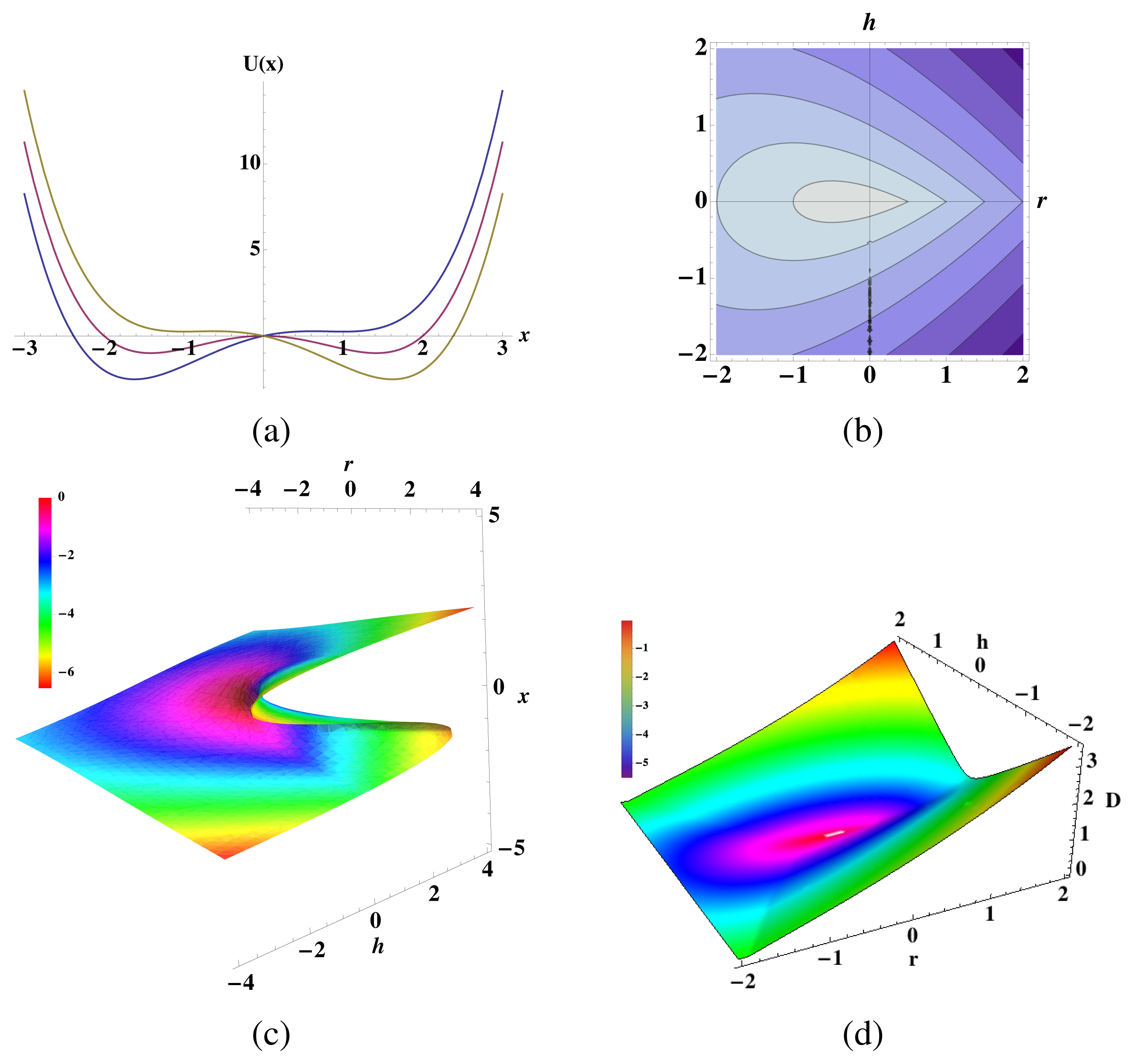
As a concrete example, consider the canonical form for the cusp catastrophe [33]:

$$\frac{dx}{dt}=h+rx-x^3+\eta (t),$$

with additive noise where 〈η(t)η(t′)〉 = 2Dδ(t− t′). The potential function is $U(x)=\frac{1}{4}{x}^4-\frac{1}{2}r{x}^2-hx$, and the corresponding bound information in the noiseless limit is:

$$\underset{D\to 0}{\text{lim}}\hspace{0.17em}{b}_{\mu }(\tau ,r,h)=\frac{\text{log\hspace{0.17em}}\sqrt{2}}{\tau }+\frac{r-3{(x^{*}(r,h))}^2}{2}.$$

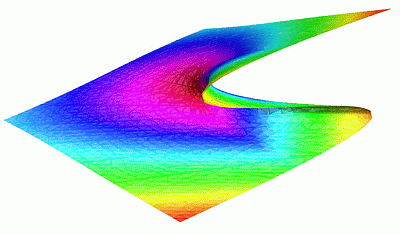
The global minimum x^*(r, h) is not everywhere differentiable in r and h, and this appears also in b_μ(τ, r, h). See Figure 3. The contour of nondifferentiability is h = 0 for r > 0. Along the contour, the potential is symmetric, there are suddenly two global minima of U(x) with $x_1^{*}=-x_2^{*}$, and so, the sign of x^* changes discontinuously across h = 0.

Interestingly, for double-well potentials and asymmetric single-well potentials, b_μ(τ) is maximized at a nonzero noise level D > 0. This is counterintuitive: adding noise only serves to decrease the process’s predictability. However, adding noise in the present affects the future in a way that cannot be predicted from the past. Since b_μ(τ) measures the amount of information shared between the present and future not shared with the past, there is a level of stochasticity that maximizes b_μ(τ) for some values of r and h. This is shown in Figure 3c.

4.2. Particles Diffusing in a Heat Bath

Suppose N particles with positions x₁, …, x_N and masses m₁, …, m_N diffuse according to the potential function U(x₁, …, x_N) in a heat bath of temperature T. Let x denote the vector of concatenated particle positions. When the inertial terms m_id²x_i/dt² are negligible, an overdamped Langevin equation can be used to approximate the particles’ trajectories:

$$\begin{array}{l}\frac{d\mathbf{x}}{dt}=\frac{1}{\gamma }{M}^{-1}\nabla U(\mathbf{x})+\eta (t)\\ \langle {\eta }_i(t)\rangle =0\\ \langle {\eta }_i(t){\eta }_j(t^{\prime })\rangle =\frac{2k_{B}T}{\gamma m_i}{\delta }_{i,j}\delta (t-t^{\prime }).\end{array}$$

M is a diagonal matrix whose entries are the particle masses, and the parameter γ is a friction coefficient that controls how strongly the particles couple to the heat bath. The stationary distribution of positions x is the Boltzmann distribution:

$${\rho }_{eq}(\mathbf{x})=\frac{1}{Z}\text{exp\hspace{0.17em}}\left(-\frac{U(\mathbf{x})}{k_{B}T}\right),$$

where Z is the partition function:

$$Z=\int \text{exp\hspace{0.17em}}\left(-\frac{U(\mathbf{x})}{k_{B}T}\right)\hspace{0.17em}d\mathbf{x}.$$

From Equation (8), the normalized single-measurement entropy is:

$$H_0=\frac{1}{\tau }\left(\frac{\langle U(\mathbf{x})\rangle }{k_{B}T}+\text{ln\hspace{0.17em}}Z\right).$$

where:

$$\langle U(\mathbf{x})\rangle =\int U(\mathbf{x})\frac{e^{-U(\mathbf{x})/k_{B}T}}{Z}d\mathbf{x},$$

which is simply proportional to the familiar definition of entropy in physics.

For notational ease, let m̄ denote the geometric mean of the masses:

$$\overline{m}={\left(\prod _{i=1}^N{m}_i\right)}^{1/N},$$

k_i the effective “spring constant” for the i^th particle:

$$k_i=\int \frac{{\partial }^{2}U(\mathbf{x})}{\partial x_i^2}\frac{e^{-U(\mathbf{x})/k_{B}T}}{Z}d\mathbf{x},$$

and ω_i the effective “oscillation frequency” for the i^th particle:

$${\omega }_i=\sqrt{k_i/m_i}.$$

From Equation (15), the entropy rate is:

$$h_{\mu }(\tau )=\frac{N\hspace{0.17em}\text{log\hspace{0.17em}}\sqrt{4k_{B}T\tau /\gamma \overline{m}}}{\tau }+\frac{\text{log\hspace{0.17em}}\sqrt{\pi e}}{\tau }-\frac{1}{2\gamma }\sum _{i=1}^N{\omega }_i^2+o(1).$$

From Equation (16), the bound information is to similar order:

$$b_{\mu }(\tau )=\frac{N\hspace{0.17em}\text{log\hspace{0.17em}}\sqrt{2}}{\tau }-\frac{1}{2\gamma }\sum _{i=1}^N{\omega }_i^2+o(1).$$

From Equation (17), the ephemeral information rate is:

$$r_{\mu }(\tau )=\frac{N\hspace{0.17em}\text{log\hspace{0.17em}}\sqrt{2k_{B}T\tau /\gamma \overline{m}}}{\tau }+\frac{\text{log\hspace{0.17em}}\sqrt{2\pi e}}{\tau }+o(1).$$

Several information measures appear dimensionally incorrect. This is a perennial concern when calculating the differential entropy of random variables that themselves have units. The probability density over those variables also has a dimension, and this leads to differential entropies that involve the log of a value with dimension. Implicitly, however, we chose a standard unit system, such that all quantities are dimensionless.

All of these quantities are extensive in N. The normalized entropy per measurement H₀ is proportional to the Boltzmann entropy by a factor of k_B/τ. The entropy rate h_μ(τ) and ephemeral information r_μ(τ) increase logarithmically with the mean squared velocity $\sqrt{\langle v^2\rangle }=k_{B}T/m$. The bound information b_μ(τ) increases when there is a larger γ. That is, it increases when there is stronger coupling between the particles and the heat bath or when there is a smaller average oscillation frequency ${\sum }_{i=1}^N{\omega }_i^2$. Since γ ≥ 0 and ${\omega }_i^2\ge 0$, the bound information is bounded above by $b_{\mu }(\tau )\le {\tau }^{-1}N\hspace{0.17em}\text{log\hspace{0.17em}}\sqrt{2}+O(\tau )$. To achieve this upper bound, the potential U(x) must be “flattened out” to decrease k_i, as described in Section 3.

There are alternative models for coupled particles diffusing in a heat bath, and there is no guarantee that even the qualitative conclusions here hold true when particle trajectories are modeled according to a second-order Langevin equation, for instance.

5. Conclusions

Our calculations led to general formulae for the information anatomy of stochastic equilibria in simple, familiar systems when the time discretization was very small. We considered a first-order nonlinear Langevin equation with a normalizable stationary distribution, invertible diffusion matrix, and analytic drift. We do not expect the expressions in Section 3 to hold for larger time discretizations, though Gaussian approximations could be used to upper bound conditional entropies more generally. We also considered first-order linear Langevin equations with normalizable stationary distribution and a noninvertible diffusion matrix in Section 3.2.

An important technical consideration is that the information anatomy of Langevin stochastic dynamics is likely not unique, just as the pre-factors for the (ε, τ)-entropy rate of an Ornstein–Uhlenbeck process depend on definition and approximation procedure [25,28]. However, further calculations give us reason to believe that the qualitative scaling seen with drift and diffusion holds regardless of the approximation method. This parallels the way that the (ε, τ)-entropy rate estimates for an Ornstein–Uhlenbeck process all increase with the diffusion coefficient. That said, a complete understanding of how information anatomy estimates vary with technique requires further study; alternatives to which the Introduction alluded. We hope that our results are sufficiently compelling to motivate further efforts.

With this caveat in mind, let us focus on qualitative rather than quantitative conclusions. Even though the entropy rate is typically viewed as a measure of randomness, some of that randomness is useful for prediction, that is, the bound information (shared between present and future, but not contained in the past), and we showed that it is sensitive to drift and the diffusion matrix. In contrast, we showed that the ephemeral information—information in the present useless for predicting or retrodicting—is sensitive only to the diffusion and not the drift. In short, for stochastic equilibria, the entropy rate consists of a quantity (ephemeral information) that has to do with a process’s inherent noisiness and a quantity (bound information) that has only to do with the underlying process regularities.

A key lesson is that information anatomy measures are sensitive to process organization. Section 3.2 showed that the divergent components of the information anatomy of linear Langevin dynamics changes discontinuously whenever one of the diffusion coefficients vanishes. This sensitivity to underlying process structure could also be a feature rather than a defect. For instance, if we know that the underlying process is a first-order linear Langevin equation, then one could infer the dimension of the deterministically evolving state space by comparing known τ-scaling relations in Section 3 with empirically determined scaling relations.

This brings us to discuss what was learned from the several example applications. Section 4.1 showed that the bound information picks up different features than one finds in a bifurcation diagram. In the noiseless limit, the cusp catastrophe b_μ is nondifferentiable on the line h = 0 for r ≥ 0, because the location of the global minimum of the potential function changes discontinuously across that contour. Moreover, this is not related to the bifurcation contour $h=\pm 2r^{3/2}/3\sqrt{3}$ [33] where the number of equilibria changes from two to one or vice versa, which has no apparent signature in the bound information. However, in these calculations, we did not avoid the “ultraviolet catastrophe”. We embraced it, since we could then evaluate the information anatomy for general nonlinear Langevin equations by linearizing. If one evaluates the information anatomies of these types of stochastic dynamics when the time discretization is not infinitesimal, however, then signatures of bifurcations should show up in the bound information as they do for the finite-time predictable information or excess entropy [16,34].

Section 4.2 calculated the information anatomy of coupled particles in a heat bath. Historically, statistical physics has been primarily concerned with H₀, the entropy of a single measurement symbol, since its changes are proportional to heat loss [35]. However, the point of this example is that alternative information-theoretic quantities capture other behavioral properties of particles diffusing in a heat bath. As an application of this analysis, it will be worth exploring how the information anatomy measures reflect the trade-off between stable information storage and heat loss in the context of Maxwell-like demons [36].

To close our discussion of applications, we briefly mention the use of information measures to express optimization principles that guide adaptive agents. A Markov process’s bound information has been used as an optimization measure called the time-local predictive information (TiPi) [12]. Moreover, the class of systems used there and for which TiPi was calculated are exactly the first-order nonlinear Langevin dynamics analyzed here. Due to the similarities in setup and approach, Appendix E compares alternative TiPi measures. Generally, an agent that wishes to maximize its TiPi will be driven into unstable regions of the potential landscape on which it diffuses. However, Appendix E shows that the similarly motivated, but alternative, optimization measures lead to different adaptive strategies. More investigation is required to compare such strategies to those seen in biological agents before general principles of adaptive behavior will be understood.

References

- Walters, P. An Introduction to Ergodic Theory; Graduate Texts in Mathematics, Volume 79; Springer-Verlag: New York, NY, USA, 1982. [Google Scholar]
- Cover, T.M.; Thomas, J.A. Elements of Information Theory, 2nd ed; Wiley-Interscience: New York, NY, USA, 2006. [Google Scholar]
- Crutchfield, J.P.; Young, K. Inferring Statistical Complexity. Phys. Rev. Lett 1989, 63, 105–108. [Google Scholar]
- Shalizi, C.R.; Crutchfield, J.P. Computational Mechanics: Pattern and Prediction, Structure and Simplicity. J. Stat. Phys 2001, 104, 817–879. [Google Scholar]
- Crutchfield, J.P.; Feldman, D.P. Regularities Unseen, Randomness Observed: Levels of Entropy Convergence. Chaos 2003, 13, 25–54. [Google Scholar]
- James, R.G.; Ellison, C.J.; Crutchfield, J.P. Anatomy of a Bit: Information in a Time Series Observation. Chaos 2011, 21, 037109. [Google Scholar]
- Palmer, S.E.; Marre, O.; Berry, M.J., II; Bialek, W. Predictive Information in a Sensory Population 2013. arXiv:1307.0225.
- Beer, R.D.; Williams, P.L. Information Processing and Dynamics in Minimally Cognitive Agents. Cogn. Sci 2014, in press. [Google Scholar]
- Tononi, G.; Edelman, G.M.; Sporns, O. Complexity and Coherency: Integrating Information in the Brain. Trends Cogn. Sci 1998, 2, 474–484. [Google Scholar]
- Strelioff, C.C.; Crutchfield, J.P. Bayesian Structural Inference for Hidden Processes. Phys. Rev. E 2014, 89, 042119. [Google Scholar]
- Sato, Y.; Akiyama, E.; Crutchfield, J.P. Stability and Diversity in Collective Adaptation. Physica D 2005, 210, 21–57. [Google Scholar]
- Martius, G.; Der, R.; Ay, N. Information driven self-organization of complex robotics behaviors. PLoS One 2013, 8, e63400. [Google Scholar]
- Varn, D.P.; Canright, G.S.; Crutchfield, J.P. Discovering Planar Disorder in Close-Packed Structures from X-Ray Diffraction: Beyond the Fault Model. Phys. Rev. B 2002, 66, 174110–174113. [Google Scholar]
- Varn, D.P.; Canright, G.S.; Crutchfield, J.P. ε-Machine spectral reconstruction theory: A direct method for inferring planar disorder and structure from X-ray diffraction studies. Acta. Cryst. Sec. A 2013, 69, 197–206. [Google Scholar]
- Crutchfield, J.P.; Young, K. Computation at the Onset of Chaos. In Entropy, Complexity, and the Physics of Information; Zurek, W., Ed.; Volume VIII, SFI Studies in the Sciences of Complexity; Addison-Wesley: Reading, MA, USA, 1990; pp. 223–269. [Google Scholar]
- Tchernookov, M.; Nemenman, I. Predictive Information in a Nonequilibrium Critical Model. J. Stat. Phys 2013, 153, 442–459. [Google Scholar]
- Atmanspracher, H.A.; Scheingraber, H. Information Dynamics; Plenum: New York, NY, USA, 1991; pp. 45–60. [Google Scholar]
- James, R.G.; Burke, K.; Crutchfield, J.P. Chaos Forgets and Remembers: Measuring Information Creation and Storage. Phys. Lett. A 2014. [Google Scholar]
- Lizier, J.; Prokopenko, M.; Zomaya, A. Information modification and particle collisions in distributed computation. Chaos 2010, 20, 037109. [Google Scholar]
- Flecker, B.; Alford, W.; Beggs, J.M.; Williams, P.L.; Beer, R.D. Partial Information Decomposition as a Spatiotemporal Filter. Chaos 2011, 21, 037104. [Google Scholar]
- Moss, F.; McClintock, P.V.E. Noise in Nonlinear Dynamical Systems; Cambridge University Press: Cambridge, UK, 1989; Volume 1. [Google Scholar]
- Shraiman, B.; Wayne, C.E.; Martin, P.C. Scaling Theory for Noisy Period-Doubling Transitions to Chaos. Phys. Rev. Lett 1981, 46, 935. [Google Scholar]
- Crutchfield, J.P.; Nauenberg, M.; Rudnick, J. Scaling for External Noise at the Onset of Chaos. Phys. Rev. Lett 1981, 46, 933. [Google Scholar]
- Girardin, V. On the Different Extensions of the Ergodic Theorem of Information Theory. In Recent Advances in Applied Probability Theory; Baeza-Yates, R., Glaz, J., Gzyl, H., Husler, J., Palacios, J.L., Eds.; Springer: New York, NY, USA, 2005; pp. 163–179. [Google Scholar]
- Gaspard, P.; Wang, X.J. Noise Chaos (ε, τ)-Entropy Per Unit Time. Phys. Rep 1993, 235, 291–343. [Google Scholar]
- Oksendal, B. Stochastic Differential Equations: An Introduction with Applications, 6th ed; Springer: New York, NY, USA, 2013. [Google Scholar]
- Yeung, R.W. Information Theory and Network Coding; Springer: New York, NY, USA, 2008. [Google Scholar]
- Gaspard, P. Brownian Motion, Dynamical Randomness, and Irreversibility. New J. Phys 2005, 7, 77–90. [Google Scholar]
- Lecomte, V.; Appert-Rolland, C.; van Wijland, F. Thermodynamic Formalism for Systems with Markov Dynamics. J. Stat. Phys 2007, 127, 51–106. [Google Scholar]
- Ellison, C.J.; Mahoney, J.R.; Crutchfield, J.P. Prediction, Retrodiction, and the Amount of Information Stored in the Present. J. Stat. Phys 2009, 136, 1005–1034. [Google Scholar]
- Crutchfield, J.P.; Ellison, C.J.; Mahoney, J.R. Time’s Barbed Arrow: Irreversibility, Crypticity, and Stored Information. Phys. Rev. Lett 2009, 103, 094101. [Google Scholar]
- Crutchfield, J.P.; Feldman, D.P. Statistical Complexity of Simple One-Dimensional Spin Systems. Phys. Rev. E 1997, 55, R1239–R1243. [Google Scholar]
- Poston, T.; Stewart, I. Catastrophe Theory and Its Applications; Pitman: London, UK, 1978. [Google Scholar]
- Feldman, D.P.; Crutchfield, J.P. Structural Information in Two-Dimensional Patterns: Entropy Convergence and Excess Entropy. Phys. Rev. E 2003, 67, 051103. [Google Scholar]
- Kittel, C.; Kroemer, H. Thermal Physics, 2nd ed; W. H. Freeman: New York, NY, USA, 1980. [Google Scholar]
- Landauer, R. Dissipation and Noise Immunity in Computation, Measurement, and Communication. J. Stat. Phys 1989, 54, 1509–1517. [Google Scholar]
- Lohr, W. Properties of the Statistical Complexity Functional and Partially Deterministic HMMs. Entropy 2009, 11, 385–401. [Google Scholar]
- Risken, H. The Fokker-Planck Equation: Methods of Solution and Applications, 2nd ed; Springer: Berlin, Germany, 1996. [Google Scholar]
- Drozdov, A.N.; Morillo, M. Expansion for the Moments of a Nonlinear Stochastic Model. Phys. Rev. Lett 1996, 77, 3280. [Google Scholar]
- Crutchfield, J.P.; Ellison, C.J.; Mahoney, J.R.; James, R.G. Synchronization and Control in Intrinsic and Designed Computation: An Information-Theoretic Analysis of Competing Models of Stochastic Computation. Chaos 2010, 20, 037105. [Google Scholar]
Figure 1.
Information anatomy of a stationary continuous-time process graphically depicted using information diagrams. Although the past entropy H[X:0] and the future entropy H[Xτ:] typically are infinite, space limitations constrain us to draw them with finite areas. (a) Information diagram for the anatomy of a process’s single observation X0 in the context of its past X:0 and its future Xτ: (after [6], with permission). (b) Information diagram for the anatomy of a Markov process, in which the present X0 causally shields the past from future. The elusive information σμ(τ) vanishes.
Figure 2.
(a) Particle diffusing according to ẋ = −x+η(t) with diffusion coefficient D = 1. A finite-time trajectory x(t) followed by the diffusing particle. (b) Over infinite time, the particle experiences positions distributed according to the probability density function ρeq(x) in Equation (7), calculated as a normalized histogram of particle positions. (c) If the previous particle position is known, a future position can be determined with less uncertainty than if no previous particle position is known. The probability Pr(x, t|0, 0) of being in position x at a time t differs from the equilibrium probability distribution ρeq(x), if we know the position of the particle at a previous time; e.g., x(0) = 0.
Figure 3.
Information anatomy of the stochastic cusp catastrophe: (a) Shifting from a double-well to single-well potentials as r and h are varied. Example potentials U(x) for various r and h: blue/dark line, r = 2 and h = −1; purple/medium line, r = 2 and h = 0; and yellow/light line, r = 2 and h = 1. (b) Contour plot of the system-dependent part of the bound information rate bμ(τ) as a function of r and h, highlighting the global minimum x* changing discontinuously as h moves through zero.
as a function of r and h: bμ(τ) is nondifferentiable with respect to h along h = 0 when r ≥ 0. (c) Bound information bμ(τ) as it varies over the cusp catastrophe equilibria surface: Height gives the fixed points as a function of r and h. Color hue is proportional to the deterministic limit
at each r and h. (d) The bound information rate is maximized at nonzero stochasticity D for double-well potentials and asymmetric single-well potentials. D maximizing
as a function of r and h: the surface is colored by
at that value of D.