Tsallis Distribution Decorated with Log-Periodic Oscillation

Abstract

In many situations, in all branches of physics, one encounters the power-like behavior of some variables, which is best described by a Tsallis distribution characterized by a nonextensivity parameter q and scale parameter T. However, there exist experimental results that can be described only by a Tsallis distributions, which are additionally decorated by some log-periodic oscillating factor. We argue that such a factor can originate from allowing for a complex nonextensivity parameter q. The possible information conveyed by such an approach (like the occurrence of complex heat capacity, the notion of complex probability or complex multiplicative noise) will also be discussed.

1. Introduction

In many situations, in all branches of physics, one encounters the behavior of some variables X, which become pure power distributions for large values of X and exponential for X → 0. Because of this, they are known as power-like distributions, and in many cases, they are identified with a Tsallis distribution [1–3],

$$F(X)=A{\left[1-(1-q)\frac{X}{T}\right]}^{1/(1-q)},$$

(1)

characterized by a scale parameter T and parameter q, known as the nonextensivity parameter (A is normalization) (the reason being the fact that Equation (1) is also emerging from nonextensive statistical mechanics [1–3]). Obviously, for X → 0, distribution Equation (1) becomes the usual Boltzmann–Gibbs exponential formula with temperature T, but it becomes pure exponential (i.e., Boltzmann–Gibbs (BG)) also for q → 1. For q ≠ 1 and large values of X, it becomes a pure power distribution that is not sensitive to scale parameter T.

To fully recognize the nontrivial character of distribution Equation (1), one must realize that, usually, in different parts of the phase space of the variable X, one encounters (or, rather, one expects) a dominance of different (if not completely disparate) dynamical factors. This is best seen in the processes of multiparticle production at high energies (the best known to us). They will serve here to exemplify our further consideration concerning some specific log-periodic oscillations, apparently visible in such processes, which must be therefore somehow be hidden in the original distribution Equation (1).

Before proceeding further, we shall briefly summarize the present status of the application of Tsallis distributions in this context, concentrating only on multiparticle production processes. They are comprised of many different mechanisms in different parts of the phase space. Limiting ourselves only to particle production in the central rapidity region and to the distribution of their transverse momenta p_T, it is customary to divide this production into independent soft and hard processes populating different parts of the transverse momentum space (A few words of definition concerning this phase space are necessary. A produced particle has some momentum $\overrightarrow{p}=[p_L,{\overrightarrow{p}}_T]$. Its longitudinal part, p_L, is defined as parallel to the axis of collision; its transverse part, ${\overrightarrow{p}}_T$ as perpendicular to that axis. They are defined by means of the rapidity y variable, $y=\frac{1}{2}\ln \frac{E+p_L}{E-p_L}$, as, respectively, $p=|\overrightarrow{p}|=m\sinh y$,whereas the energy of the particle, $E=\sqrt{m^2+p^2}=m\cosh y$. Central rapidity means y = 0. In what follows, our X from Equation (1) will be identified with transverse momentum, X = p_T.) separated by a momentum scale p₀. As a rule of thumb, the spectra of the soft processes in the low-p_T region are (almost) exponential, F(p_T)~exp(−p_T/T) and are usually associated with the thermodynamical description of the hadronizing system. The p_T spectra of the hard process in the high-p_T region are regarded as essentially power-like, $F(p_T)~p_T^{-n}$, and are usually associated with the hard scattering process (for relevant literature concerning both parts, see [4]). However, it was very soon recognized that both descriptions could be replaced by a simple interpolating formula [5,6],

$$F(p_T)=A{\left(1+\frac{p_T}{p_0}\right)}^{-n},$$

(2)

that becomes power-like for high p_T and exponential-like for low p_T. The reasoning was that for high p_T, where we are usually neglecting the constant term, the scale parameter p₀ becomes irrelevant, whereas for low p_T, it becomes, together with the power index n, an effective temperature T = p₀/n. The same formula re-emerged later to become known as the QCD-based Hagedorn formula [7]. It was used for the first time in [8] and became one of the standard phenomenological formulas for p_T data analysis [9–17]. In the mean time, it was realized that both formulas are, in fact, identical, once:

$$\begin{array}{ccc}n=\frac{1}{q-1}& \mathrm{and}& p_0=nT\end{array},$$

(3)

and therefore, they can be used interchangeably (both Equations (1) and (2) have been widely used in the phenomenological analysis of multiparticle productions, including situations where the nowadays observed spectra extend over many orders of magnitude, [9–42]. Up to now, such a possibility of testing the Tsallis distribution offered only cosmic ray fluxes; cf. [43–45].

This distribution is usually used in a thermodynamical contextin which the scale parameter T is identified with the usual temperature (although such an identification cannot be solid [46–50]) and with a real power index n = 1/(q−1) (or a real nonextensivity parameter q). Actually, a Tsallis distribution can be regarded as a generalization to the real power n (or q) of such well-known distributions as the Snedecor distribution (with n = (ν + 2)/2 and integer ν, which, for ν →∞, it becomes an exponential distribution).

In [51–53], we investigate the case when q is a complex number. We shall review our results in this field in the next section, adding examples where log-periodic oscillations occur at different energies and for different collision systems. In Section 3, we discuss the possible consequences of the complex nonextensivity parameter, including some new recent developments in this field (as complex probability and complex multiplicative noise). The final section contains our conclusions and summary.

2. Log-Periodic Oscillations in a Tsallis Distribution: Complex Power Index

Recently, the experiments [12–17] at the Large Hadron Collider (LHC) at CERN provided new data in a very large domain of transverse momenta, p_T, phase space. They turned out to be extremely interesting because of the following:

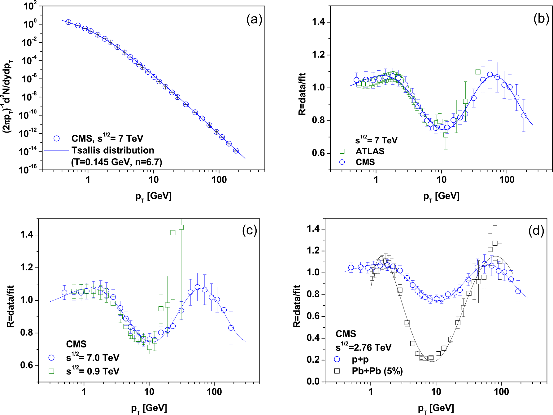
• They allow us to test the standard Tsallis formula, Equation (1), over ~14 orders of magnitude. As can be seen in Figure 1a, the observed p_T distributions of secondaries produced in proton-proton collisions in these experiments can be very well reproduced (cf. also [40,41]) (these secondaries were produced at midrapidity, i.e., for y ≃ 0, for which, for a large transverse momentum, p_T > m (where m is the mass of the particle), one has that, approximately, the energy of particle E ≃ p_T, i.e., it practically coincides with p_T.).
• Additionally, what is of special importance to us is that they disclose some features that suggest a departures from the single form of Equation (1); cf. Figure 1b,c. Apparently, they could not be seen in previous experiments, because they seem to be connected with rather large values of transverse momenta, which are not available earlier.

However, whereas fits to Equation (1) look fairly good, closer inspection shows that the ratio of data/fit is not flat. It shows some kind of visible oscillations; cf. Figure 1b. These are the oscillations we have mentioned before.

It turns out that these oscillations cannot be compensated, or erased, by any reasonable change of fitting parameters. Moreover, they are visible by all three experiments, CMS, ATLAS and ALICE. The only condition for such an effect to be visible is that the experiment covers a sufficiently large domain of transverse momenta p_T; cf. Figure 1b. It is also seen at all energies covered by these experiments; cf. Figure 1c. Finally, as Figure 1d shows, this effect is also visible (and is even more pronounced) in nuclear collisions. When taken seriously, it turns out that to account for these oscillations, one has to “decorate” distribution f (p_T ) from Equation (1) (i.e., one has to multiply it) with some log-periodic oscillating factor. It is is usually taken in the form [56]:

$$R(E)=a+b\cos \left[c\ln (E+d)+f\right].$$

(4)

Before proceeding any further, let us remember that such log-periodic oscillations are widely know in all situations in which one encounters power distributions. In fact, such behavior has been found in earthquakes [57,58], escape probabilities in chaotic maps close to a crisis [59], biased diffusion of tracers on random systems [60–62], kinetic and dynamic processes on random quenched and fractal media [63–66], when considering the specific heat associated with self-similar [67] or fractal spectra [68], diffusion-limited-aggregate clusters [69], growth models [70] or stock markets near financial crashes [71–74], to name only a few examples. However, in all of these cases, the basic distributions were a scale-free power laws, without any scale parameter (here T) and without a constant term governing their X < nT behavior.

In the context of nonextensive statistical mechanics, log-periodic oscillations have first been observed and discussed while analyzing the convergence dynamics of z-logistic maps [75]. In this paper, we shall propose another way of introducing such oscillations to Tsallis distributions. It will be based on allowing the power index n (or nonextensivity parameter q) in a Tsallis distribution to become complex. For the completeness of the presentation, we start from the simple pure power law distribution,

$$O(x)=C\cdot x^{-m}.$$

(5)

This function is scale invariant, i.e.,

$$O(\lambda x)=\mu O(x),$$

(6)

with m = ln μ/ln λ. However, because 1 = exp (ι2πk), one can as well write that

$$\begin{array}{cc}\mu {\lambda }^m=1=\exp (\iota 2\pi k),& k=0,1,\dots \end{array}$$

(7)

This means, therefore, that, in general, the index m can become complex,

$$m=-\frac{\ln \mu }{\ln \lambda }+\iota \frac{2\pi k}{\ln \lambda }.$$

(8)

As will be obvious from further, general considerations, such a form of the power index results in R, as given by Equation (4), when one only keeps k = 0, 1 terms (which is the usual assumption customarily applied in all applications [56,57,59,60,63]).

However, the Tsallis distribution is only a power-like, not a power, distribution. Therefore, to explain the origin of such a dressing factor in this case, one has to find the right variable in which the real scaling holds. We start from the observation that, whereas the BG distribution,

$$f(E)=\frac{1}{T}\exp \left(-\frac{E}{T}\right),$$

(9)

comes from the simple equation,

$$\frac{df(E)}{dE}=-\frac{1}{T}f(E)$$

(10)

with the scale parameter T being constant, the same equation, but with a variable scale parameter in the form:

$$T=T(E)=T_o+\frac{E}{n},$$

(11)

(known as preferential attachment in networks [22,76,77] (it is worth recalling here that this very same form, T (E) = T₀ + (1 − q)E, also appears in [39] within a Fokker–Planck dynamics applied to the thermalization of quarks in a quark-gluon plasma by collision processes)),

$$\frac{df(E)}{dE}=-\frac{1}{T(E)}f(E)=-\frac{1}{T_o+E/n}f(E),$$

(12)

results in the Tsallis distribution:

$$f(E)=\frac{n-1}{n{T}_o}{\left(1+\frac{E}{n{T}_o}\right)}^{-n}.$$

(13)

We shall write now Equation (12) in finite difference form,

$$f(E+\delta E)=\frac{-n\delta E+nT+E}{nT+E}f(E).$$

(14)

In a practical sense, this means a first-order Taylor expansion for small E << E (from Equation (14) on, we use T instead of T₀). We shall now consider a situation in which E always remains finite (albeit, depending on the value of the new scale parameter α, it can be very small) and equal to:

$$\delta E=\alpha nT(E)=\alpha (nT+E).$$

(15)

Because one expects that changes δE are of the order of the temperature T, the scale parameter must be limited by 1/n, i.e., < 1=n. In this case, substituting Equation (15) into Equation (14), we have,

$$f[E+\alpha (nT+E)]=(1-\alpha n)f(E).$$

(16)

Expressing Equation (16) in a new variable x,

$$x=1+\frac{E}{nT},$$

(17)

we recognize that the argument of the function on the left-hand side of equality Equation (16) is:

$$E+\alpha (nT+E)=(1+\alpha )xnT-nT,$$

while the argument of the function on its right-hand side is:

$$E=xnT-nT.$$

Notice that, in comparison with the right-hand side, the variable x on the left-hand side is multiplied by the additional factor (1 + α). This means that, formally, Equation (16), when expressed in x, corresponds to the following scale-invariant relation:

$$g[(1+\alpha )x]=(1-\alpha n)g(x).$$

(18)

This means that, following the discussion after Equation (6), its general solution is a power law,

$$g(x)=x^{-m_k},$$

(19)

with exponent m_k depending on α and acquiring an imaginary part,

$$m_k=-\frac{\ln (1-\alpha n)}{\ln (1+\alpha )}+ik\frac{2\pi }{\ln (1+\alpha )}.$$

(20)

The special case of k = 0, i.e., the usual real power law solution with m₀ corresponding to fully-continuous scale invariance (in this case, power law exponent m₀ still depends on α and increases with it roughly as $m_0\simeq n+\frac{n}{2}(n+1)\alpha +\frac{n}{12}(4n^2+3n-1){\alpha }^2+\frac{n}{24}(6n^3+4n^2-n+1){\alpha }^3+\dots$; notice also that α < 1/n), recovers in the limit α → 0 the power n in the usual Tsallis distribution. In general, one has:

$$g(x)={\displaystyle \sum _{k=0}{w}_k}\cdot \mathrm{Re}(x^{-m_k})=x^{-\mathrm{Re}(m_k)}{\displaystyle \sum _{k=0}{w}_k}\cdot \cos [\mathrm{Im}(m_k)\ln (x)].$$

(21)

One therefore obtains a Tsallis distribution decorated by a weighted sum of log-oscillating factors (where x is given by Equation (17)). Because, usually, in practice, we do not a priori know the details of the dynamics of processes under consideration (i.e., we do not known the weights w_k), for fitting purposes, one usually uses only k = 0 and k = 1. In this case, one has, approximately,

$$g(E)\simeq {\left(1+\frac{E}{nT}\right)}^{-m_0}\left\{w_0+w_1\cos \left[\frac{2\pi }{\ln (1+\alpha )}\ln \left(1+\frac{E}{nT}\right)\right]\right\}$$

(22)

and reproduces the general form of a dressing factor given by Equation (4) and often used in the literature [56]. In this approximation, the parameters a, b, c, d and f from Equation (4) get the following meaning:

$$\begin{array}{cccc}\frac{a}{b}=\frac{w_0}{w_1},& c=\frac{2\pi }{\ln (1+\alpha )},& d=nT,& f=-\frac{2\pi }{\ln (1+\alpha )}\ln (nT).\end{array}$$

(23)

In fact, this is not the most general result, for in our derivation, Equations (15)–(18)), we have so far only accounted for a single-step evolution. In a real situation, one should expect to have a whole hierarchy of evolutions. In such a case, consecutive steps of evolution are connected by:

$$E_i=E_{i-1}+{\alpha }_{i-1}(nT+E_{i-1}),$$

(24)

each with its own scale parameter _i. In the simplest situation, neglecting any fluctuations of consecutive scaling parameters, i.e., assuming that all α_i = α, one has that after k steps:

$$nT+E_k={(1+a)}^k(nT+E_0).$$

(25)

This means that, in general, Equation (18) should be replaced by a new scale-invariant equation:

$$g[{(1+\alpha )}^{k}x]={(1-\alpha n)}^{k}g(x).$$

(26)

whereas this equation does not change the slope parameter m₀, it significantly influences the frequency of oscillations, which are now times smaller,

$$c=\frac{2\pi }{k\ln (1+\alpha )}$$

(27)

(in Equation (26) λ = (1+α)^k and μ = (1−αn)^k ; the slope parameter m₀ = −ln μ/ln λ is independent of k, whereas the frequency of oscillations, 2π/ln λ, decreases with k as 1/k). For a more complex behavior of intermediate scale parameters _i, one gets more complicated expressions (we shall not discuss this here).

3. Other Consequences of the Complex Nonextensivity Parameter

There are other consequences of allowing the parameter m to be complex. In what follows, we shall discuss briefly three examples: complex heat capacity, complex probability and complex multiplicative noise.

3.1. Complex Heat Capacity

The complex power exponent in the Tsallis distribution, m = m′ + i · m″, means that:

$$q-1=\frac{1}{m}=\frac{m^{\prime }}{{|m|}^2}+i\frac{m^{″}}{{|m|}^2}.$$

(28)

As shown in [29] (cf., also, [22,23,78–80]), the nonextensivity parameter q can be treated as a measure of the thermal bath heat capacity C with:

$$C=\frac{1}{q-1}=m^{\prime }+i{m}^{″}.$$

(29)

The complex nonextensive parameter q must therefore have some profound consequences, because now, the corresponding heat capacity becomes complex, as well. As a matter of fact, such complex (frequency dependent) heat capacities (or generalized calorimetric susceptibilities) are known in the literature [87,88] and are usually written in the form:

$$C=C_{\infty }+\frac{C_0-C_{\infty }}{1+{(\omega \tau )}^2}(1-i\omega \tau ).$$

(30)

Here, C_∞ is the heat capacity related to the infinitely fast degrees of freedom of the system as compared to the frequency ω, and C₀ is the total contribution at equilibrium (the frequency is set to zero) of the degrees of freedom, fast and slow, of the sample. The time constant τ is the kinetic relaxation time constant of a certain internal degree of freedom.

These complex heat capacities are known as dynamic heat capacities and are intensively explored from both experimental and theoretical perspectives. It is expected that dynamic calorimetry can provide an insight into the energy landscape dynamics; cf., for example, [89–92]. Usually, one associates the imaginary part of linear susceptibility with the absorption of energy by the sample from the applied field.

In the case of temperature fluctuations δT(t), the deviation of the energy from its equilibrium value δU(t) is, for a certain linear operator Ĉ(t), some linear function of the corresponding variation of the temperature,

$$\delta U(t)=\widehat{C}\delta T(t).$$

(31)

If the temperature of the reservoir changes infinitely slowly in time, then the system can keep up with any changes in the reservoir, and its susceptibility is just the specific heat of the system C_V. However, in general, the behavior of the system is described by a generalized susceptibility C_V(ω), which can be called the complex and ω-dependent heat capacity of the system. The change in the energy of a system in the field of the thermal force can be represented by:

$$\delta U(t)={\displaystyle \int L}(t^{\prime })\delta T(t-t^{\prime })d{t}^{\prime },$$

(32)

where L(t′) is the response function of the system describing its relaxation properties given by $\Phi (t)={\displaystyle {\int }_t^{\infty }L}(t^{\prime })d{t}^{\prime }$. Taking the Fourier transform, one gets:

$$\delta U(\omega )=C_V(\omega )\delta T(\omega ),$$

(33)

where:

$$C_V(\omega )={\displaystyle \int L}(t^{\prime })e^{i\omega t^{\prime }}d{t}^{\prime }$$

(34)

is the generalized susceptibility of the system and is called the complex heat capacity. In practice, the frequency-dependent heat capacity is a linear susceptibility describing the response of the system to the small thermal perturbation (occurring on the time scale 1/ω) that takes the system slightly away from the equilibrium.

A complex C_V (ω) means that δU and δT are shifted in phase and that the entropy production in the system differs from zero [92]. The corresponding fluctuation-dissipation theorem for the frequency-dependent heat capacity was established in [91]. According to this result, the frequency-dependent heat capacity may be expressed within the linear response approximation as a linear susceptibility describing the response of the system to arbitrarily small temperature perturbations away from equilibrium,

$$C_V(\omega )=\frac{{\langle U^2\rangle }_0}{{\langle T\rangle }^2}-i\frac{\omega }{{\langle T\rangle }^2}{\displaystyle {\int }_0^{\infty }dt{e}^{-i\omega t}}\langle U(0)U(t)\rangle$$

(35)

(the ω denotes the frequency with which the temperature field is varying with time).

The above results for heat capacity can now be used for a new phenomenological interpretation of the complex q parameter discussed before. Namely, one can argue that:

$$q-1=\frac{Var(T)}{{\langle T\rangle }^2}-i\frac{S(T)}{{\langle T\rangle }^2},$$

(36)

where:

$$S(T)=\omega {\displaystyle \int C}ov[T(0),T(t)]e^{-i\omega t}dt$$

(37)

is the spectral density of temperature fluctuations (i.e., the Fourier transform of the covariance function averaging over the nonequilibrium density matrix).

We would like to stress at this point that, in a sense, Equation (36) can be regarded as a generalization of our old proposition for interpreting q as a measure of non-statistical intrinsic fluctuations in the system Equation [83–86] (which corresponds to the real part of Equation (36)) by adding the effect of the spectral density of such fluctuations (via the imaginary part of Equation (36)). Notice that Equation (36) follows from Equation (29) and the relation U = C_VT, allowing one to write Equation (35) in the form of Equation (36).

3.2. Complex Probability

From the point of view of superstatistics [81–85], in our particular case, complex parameter q corresponds to a complex probability distribution. Namely, one uses the property that gamma-like fluctuation of the scale parameter T in an exponential BG distribution Equation (9) results in the q-exponential Tsallis distribution Equation (1) with q > 1. The parameter q is given here by the strength of these fluctuations, q = 1 + V ar(X)/<X>². From the thermal perspective, it corresponds to the situation in which the heath bath is not homogeneous, but has different temperatures in different parts, which are fluctuating around some mean temperature T₀. It must be therefore described by two parameters: a mean temperature T₀ and the mean strength of fluctuations given by q.

We now perform the same procedure, but using two gamma distributions, one with a real power index, m₀ − 1, and one with a complex power index, m₀ + im₁ −1,

$$\begin{array}{l}g(1/T)=w_0\frac{1}{\Gamma (m_0)}n{T}_0{\left(n\frac{T_0}{T}\right)}^{m_0-1}\exp \left(-n\frac{T_0}{T}\right)+\\ +w_1\frac{1}{\Gamma (m_0+i{m}_1)}n{T}_0{\left(n\frac{T_0}{T}\right)}^{m_0+i{m}_1-1}\exp \left(-n\frac{T_0}{T}\right).\end{array}$$

(38)

As the result, one gets a complex distribution (complex pdf):

$$h_q(E)={\displaystyle {\int }_0^{\infty }f(E)g(1/T)d(1/T)=C{w}_0}{\left(1+\frac{E}{n{T}_0}\right)}^{-m_0}+C{w}_1{\left(1+\frac{E}{n{T}_0}\right)}^{-m_0-i{m}_1},$$

(39)

the real part of which is the pdf in the form of a Tsallis distribution decorated with log-periodic oscillations of the type of Equation (22),

$$\mathrm{Re}[h_q(E)]=C{\left(1+\frac{E}{n{T}_0}\right)}^{-m_0}\cdot \left\{w_0+w_1\cos \left[m_1\ln \left(1+\frac{E}{n{T}_0}\right)\right]\right\}.$$

(40)

The complex pdf has a number of interesting properties [93–96]. It plays an important role in the interference among resonance states during scattering experiments. It is associated with the phase of the resonance channel probability amplitudes (in non-Hermitian quantum mechanics). In wireless communication systems, it is generated by a superposition of finite random variables and usually involves movement, scattering, diffusion or diffraction. The imaginary part is proportional to the degree of the correlation. The imaginary part is then a function of a correlation coefficient or other parameters that state the degree of the relationship of each individual random variable of the superposition of the random variable having a complex pdf. The real and imaginary part have diverse properties, i.e., one for the real valued pdf and the other for the elementary correlation, respectively.

It is interesting to note that entropy:

$$H=-\left|{\displaystyle \int {\displaystyle \int (a\ln a+i\cdot b\ln b)d{x}_{1}d{x}_2}}\right|=$$

(41)

corresponding to complex joint probability,

$$f(x_1,x_2)=a(x_1,x_2)+i\cdot b(x_1,x_2),$$

(42)

consists of two components:

$$\begin{array}{ccc}{H}_1=-{\displaystyle \int {\displaystyle \int a\ln ad{x}_{1}d{x}_2},}& H_2=-{\displaystyle \int {\displaystyle \int b\ln bd{x}_{1}d{x}_2};}& H=|H_1+i{H}_2|\sqrt{H_1^2+H_2^2}\end{array}\ge H_1.$$

(43)

The imaginary part of entropy is proportional to the degree of incompatibility of the correlated stochastic processes. The incompatibility increases the entropy of correlated stochastic processes.

3.3. Complex Multiplicative Noise

It is known that multiplicative noise leads to a Tsallis distribution [86]. It is then natural to expect that multiplicative complex noise should result in complex q and in log-periodic oscillations in Tsallis distributions. This can be defined by a Langevin equation:

$$\begin{array}{ccc}\frac{dp}{dt}+\gamma (t)p=\xi (t),& \mathrm{where}& \gamma (t)={\gamma }_0(t)+i{\gamma }_1.\end{array}$$

(44)

The resulting distribution [86] is now:

$$\begin{array}{cccc}f(p)={\left(1+\frac{q-1}{T}{p}^2\right)}^{\frac{q}{q-1}}& \mathrm{where}& T=\frac{2Var(\xi )}{\langle \gamma \rangle },& q=1+\frac{2Var(\gamma )}{\langle \gamma \rangle }.\end{array}$$

(45)

The parameter q is now complex, because 〈γ〉 is complex. Even more importantly, (q − 1)/T = V ar(γ)/V ar(ξ) is real (it tends to zero for q → 1). This is because the complex term γ₁ added to the noise is constant. Notice that we could just as well replace in Equation (45) (q − 1) (p²/T) by $(p^2/p_0^2)$, where $p_0^2=Var(\xi )/Var(\gamma )$. The examples and discussion of the systems characterized by the appearance of “imaginary” multiplicative noise terms in an effective Langevin-type description can be found in [97] (In fact, this is not exactly the Tsallis formula from Equation (1). To get it, one has to allow for correlation between noises and the drift term due to additive noise, i.e., for Cov(ξ,γ) ≠ 0 and 〈ξ〉 ≠ 0 (see [98] for details). One obtains then Equation (1), but with, in general, complex T = T (q). We shall not discuss it here.).

4. Summary and Conclusions

In many places in physics, and especially in the realm of high energy multiparticle production processes that we are particularly interested in, it became a standard procedure to fit the data on transverse momentum distributions by means of the quasi-power Tsallis formula. The usual interpretation in such cases is that the scale parameter T is a kind of “temperature”, whereas additional nonextensivity parameter q describes intrinsic, non-statistical fluctuations existing in the system [18–39,43,81–86,98]. However, with the increasing range of transverse momenta measured in recent experiments [12–17], two things happened:

• They still can be fitted by the same formula (which came as a surprise, because fits now cover ~14 orders of magnitude of the measured cross-sections [4,40–42]).
• New data was revealed to be weak, but persistent oscillation of the log-periodic character (already discussed briefly in [51–53]).

If taken seriously, such log-periodic structures in the data indicate that the system and/or the underlying physical mechanisms have the characteristic scale-invariant behavior. This is interesting, as it provides important constraints on the underlying physics. The presence of log-periodic features signals the existence of important physical structures hidden in the fully scale-invariant description. It is important to recognize that Equation (12) represents an averaging over highly “non-smooth” processes and, in its present form, suggests a rather smooth behavior. In reality, there is a discrete time evolution for the number of steps. To account for this fact, one replaces a differential Equation (10) by a difference quotient and expresses dt as a discrete step approximation given by Equation (15), with parameter being a characteristic scale ratio. It can also be shown that discrete scale invariance and its associated complex exponents can appear spontaneously, without a pre-existing hierarchical structure. Finally, a complex nonextensivity parameter promises new perspectives in future phenomenological applications being connected to complex heat capacity, to the notion of complex probability or to complex multiplicative noise, to mention only a few examples discussed briefly in our paper.

References

- Tsallis, C. Possible generalization of Boltzmann-Gibbs statistics. J. Stat. Phys. 1998, 52, 479–487. [Google Scholar]
- Tsallis, C. Nonadditive entropy: The concept and its use. Eur. Phys. J. A. 2009, 40, 257–266. [Google Scholar]
- Tsallis, C. Introduction to Nonextensive Statistical Mechanics; Springer: New York, NY, USA, 2009. [Google Scholar]
- Wong, C.-Y.; Wilk, G.; Cirto, L.J.L.; Tsallis, C. Possible Implication of a Single Nonextensive pT Distribution for Hadron Production in High-Energy pp Collisions 2014, arXiv, 1412.0474.
- Michael, C.; Vanryckeghem, L. Consequences of momentum conservation for particle production at large transverse momentum. J. Phys. G. 1977, 3, L151–L156. [Google Scholar]
- Michael, C. Large transverse momentum and large mass production in hadronic interactions. Prog. Part. Nucl. Phys. 1979, 2, 1–39. [Google Scholar]
- Hagedorn, R. Multiplicities, pT distributions and the expected hadron → quark-gluon phase transition. Riv. Nuovo Cimento 1983, 6, 1–50. [Google Scholar]
- Arnison, G.; Astbury, A.; Aubert, B.; Bacci, C.; Bernabei, R.; Bézaguet, A.; Böck, R.; Bowcock, T. J. V.; Calvetti, M.; Carroll, T.; et al.; UA1 Collab Transverse momentum spectra for charged particles at the CERN proton-antiproton collider. Phys. Lett. B. 1982, 118, 167–172. [Google Scholar]
- Adare, A.; Aanasiev, S.; Aidala, C.; Ajitanand, N.N.; Akiba, Y.; Al-Bataineh, H.; Alexander, J.; Aoki, K.; Aphecetche, L.; Armendariz, R.; Catzb, P.; et al.; PHENIX Collaboration Measurement of neutral mesons in p + p collisions at GeV and scaling properties of hadron production. Phys. Rev. D. 2011, 83, 052004:1–052004:26. [Google Scholar]
- Adare, A.; Aanasiev, S.; Aidala, C.; Ajitanand, N.N.; Akiba, Y.; Al-Bataineh, H.; Alexander, J.; Aoki, K.; Aphecetche, L.; Armendariz, R.; Catzb, P.; et al. (PHENIX Collaboration). Identified charged hadron production in p + p collisions at and 62.4 GeV. Phys. Rev. C. 2011, 83, 064903:1–64903:29. [Google Scholar]
- Adams, J.; Aggarwal, M. M.; Ahammed, Z.; Amonett, J.; Anderson, B. D.; Anderson, M.; Arkhipkin, D.; Averichev, G. S.; Y. Bai, Y.; J. Balewski, J.; et al.; STAR Collaboration Multiplicity dependence of inclusive pt spectra from p-p collisions at GeV. Phys. Rev. D. 2006, 74, 032006:1–032006:17. [Google Scholar]
- Khachatryan, V.; Sirunyan, A. M.; Tumasyan, A.; Adam, W.; Bergauer, T.; Dragicevic, M.; Erö, J.; Friedl, M.; Frühwirth, R; Ghete, V. M.; et al.; CMS Collaboration Transverse-momentum and pseudorapidity distributions of charged hadrons in pp collisions at and 2: 36 TeV. JHEP 2010, 2, 041:1–041:19. [Google Scholar]
- Chatrchyan, S.; Khachatryan, V.; Sirunyan, A. M.; Tumasyan, A.; Adam, W.; Bergauer, T.; Dragicevic, M.; Erö, J.; Fabjan, C.; Friedl, M.; et al. (CMS Collaboration). Charged particle transverse momentum spectra in pp collisions at and 7 TeV. JHEP 2011, 8, 086:1–086:38. [Google Scholar]
- Khachatryan, V.; Sirunyan, A. M.; Tumasyan, A.; Adam, W.; Bergauer, T.; Dragicevic, M.; Erö, J.; Fabjan, C.; Friedl, M; Fruhwirth, ¨ R; et al.; CMS Collaboration Transverse-Momentum and Pseudorapidity Distributions of Charged Hadrons in pp Collisions at TeV. Phys. Rev. Lett. 2010, 105, 022002:1–022002:5. [Google Scholar]
- Aad, G.; Abbott, B.; Abdallah, J.; Abdelalim, A. A.; Abdesselam, A.; Abdinov, O.; Abi, B.; Abolins, M.; Abramowicz, H.; Abreu, H.; et al.; ATLAS Collaboration Charged-particle multiplicities in pp interactions measured with the ATLAS detector at the LHC. New J. Phys. 2011, 13, 053033:1–053033:67. [Google Scholar]
- Aamodt, K.; Abel, N.; Abeysekara, U.; Abrahantes Quintana, A.; Abramyan, A.; Adamová, D.; Aggarwal, M. M.; Aglieri Rinella, G.; Agocs, A. G.; Aguilar Salazar, S.; et al.; ALICE Collaboration Transverse momentum spectra of charged particles in proton-proton collisions at GeV with ALICE at the LHC. Phys. Lett. B. 2010, 693, 53–68. [Google Scholar]
- Aamodt, K.; Abrahantes Quintana, A.; Adamová, D.; Adare, A. M.; Aggarwal, M. M.; Aglieri Rinella, G.; Agocs, A. G.; Aguilar Salazar, S.; Ahammed, Z.; Ahmad, N.; et al.; ALICE Collaboration Strange particle production in proton-proton collisions at with ALICE at the LHC. Eur. Phys. J. C. 2011, 71, 1594:1–1594:24. [Google Scholar]
- Bediaga, I.; Curado, E.M.F.; de Miranda, J.M. A nonextensive thermodynamical equilibrium approach in e+e− → hadrons. Physica A 2000, 286, 156–163. [Google Scholar]
- Beck, C. Non-extensive statistical mechanics and particle spectra in elementary interactions. Physica A 2000, 286, 164–180. [Google Scholar]
- Wilk, G.; Włodarczyk, Z. Power laws in elementary and heavy-ion collisions. Eur. Phys. J. A. 2009, 40, 299–312. [Google Scholar]
- Rybczyński, M.; Włodarczyk, Z. Tsallis statistics approach to the transverse momentum distributions in p – p collisions. Eur. Phys. J. C. 2014, 74, 2785:1–2785:5. [Google Scholar]
- Wilk, G.; Włodarczyk, Z. Consequences of temperature fluctuations in observables measured in high-energy collisions. Eur. Phys. J. A. 2012, 48, 161:1–161:13. [Google Scholar]
- Wilk, G.; Włodarczyk, Z. The imprints of superstatistics in multiparticle production processes. Cent. Eur. J. Phys. 2012, 10, 568–575. [Google Scholar]
- Wibig, T. The non-extensivity parameter of a thermodynamical model of hadronic interactions at LHC energies. J. Phys. G. 2010, 37, 115009:1–115009:4. [Google Scholar]
- Wibig, T. Constrains for non-standard statistical models of particle creations by identified hadron multiplicity results at LHC energies. Eur. Phys. J. C. 2014, 74, 2966:1–2966:8. [Google Scholar]
- Ürmössy, K.; Barnaföldi, G.G.; Biró, T.S. Generalised Tsallis statistics in electron-positron collisions. Phys. Lett. B. 2011, 701, 111–116. [Google Scholar]
- Ürmössy, K.; Barnaföldi, G.G.; Biró, T.S. Microcanonical jet-fragmentation in proton-proton collisions at LHC energy. Phys. Lett. B. 2012, 718, 125–129. [Google Scholar]
- Biró, T.S.; Barnaföldi, G.G.; Van, P. New entropy formula with fluctuating reservoir. Physica A 2015, 417, 215–220. [Google Scholar]
- Biró, T.S.; Barnaföldi, G.G.; Van, P. Quark-gluon plasma connected to finite heat bath. Eur. Phys. J. C. 2013, 49, 110:1–110:5. [Google Scholar]
- Cleymans, J.; Worku, D. The Tsallis distribution in proton-proton collisions at TeV at the LHC. J. Phys. G. 2012, 39, 025006:1–025006:12. [Google Scholar]
- Cleymans, J.; Worku, D. Relativistic thermodynamics: Transverse momentum distributions in high-energy physics. Eur. Phys. J. A. 2012, 48, 160:1–160:8. [Google Scholar]
- Azmi, M.D.; Cleymans, J. Transverse momentum distributions in proton-proton collisions at LHC energies and Tsallis thermodynamics. J. Phys. G. 2014, 41, 065001:1–065001:10. [Google Scholar]
- Deppman, A. Properties of hadronic systems according to the nonextensive self-consistent thermodynamics. J. Phys. G. 2014, 41, 055108–055108:10. [Google Scholar]
- Sena, I.; Deppman, A. Systematic analysis of pT -distributions in p + p collisions. Eur. Phys. J. A. 2013, 49, 17:1–17:5. [Google Scholar]
- Marques, L.; Andrade-II, E.; Deppman, A. Nonextensivity of hadronic systems. Phys. Rev. D. 2013, 87, 114022:1–114022:6. [Google Scholar]
- Khandai, P.K.; Sett, P.; Shukla, P.; Singh, V. Hadron spectra in p + p collisions at RHIC and LHC energies. Int. J. Mod. Phys. A 2013, 28, 1350066:11350066:12. [Google Scholar]
- Khandai, P.K.; Sett, P.; Shukla, P.; Singh, V. System size dependence of hadron pT spectra in p + p and Au + Au collisions at GeV. J. Phys. G. 2014, 41, 025105:1–025105:10. [Google Scholar]
- Li, B.C.; Wang, Y.-Z.; Liu, F.-H. Formulation of transverse mass distributions in Au – Au collisions at GeV/nucleon. Phys. Lett. B. 2013, 725, 352–356. [Google Scholar]
- Walton, D.B.; Rafelski, J. Equilibrium distribution of heavy quarks in Fokker-Planck dynamics. Phys. Rev. Lett. 2000, 84, 31–34. [Google Scholar]
- Wong, C.Y.; Wilk, G. Tsallis Fits to pT Spectra for pp Collisions at the LHC. Acta Phys. Pol. B. 2012, 43, 2047–2054. [Google Scholar]
- Wong, C.Y.; Wilk, G. Tsallis fits to pT spectra and multiple hard scattering in pp collisions at the LHC. Phys. Rev. D. 2013, 87, 114007:1–114007:19. [Google Scholar]
- Wong, C.Y.; Wilk, G. Relativistic Hard-Scattering and Tsallis Fits to pT Spectra in pp Collisions at the LHC 2013, arXiv, 1309.7330.
- Beck, C. Generalized statistical mechanics of cosmic rays. Physica A 2004, 331, 173–181. [Google Scholar]
- Tsallis, C.; Anjos, J.C.; Borges, E.P. Fluxes of cosmic rays: A delicately balanced stationary state. Phys. Lett. A. 2003, 310, 372–376. [Google Scholar]
- Wilk, G.; Włodarczyk, Z. Nonextensive thermal sources of cosmic rays. Cent. Eur. J. Phys. 2010, 8, 726–738. [Google Scholar]
- Tsallis, C. Non-extensive thermostatistics: Brief review and comments. Physica A 1995, 221, 277–290. [Google Scholar]
- Rios, L.A.; Galvão, R.M.O.; Cirto, L. Comment on “Debye shielding in a nonextensive plasma”. Phys. Plasmas. 2012, 19, 034701:1–034701:3. [Google Scholar]
- Andrade, J.S.; da Silva, G.F.T.; Moreira, A.A.; Nobre, F.D.; Curado, E.M.F. Thermostatistics of Overdamped Motion of Interacting Particles. Phys. Rev. Lett. 2010, 105, 26060:1–26060:4. [Google Scholar]
- Andrade, R.F.S.; Souza, A.M.C.; Curado, E.M.F.; Nobre, F.D. A thermodynamical formalism describing mechanical interactions. Europhys. Lett. 2014, 108, 20001:1–20001:6. [Google Scholar]
- Curado, E.M.; Souza, A.M.; Nobre, F.D.; Andrade, R.F. Carnot cycle for interacting particles in the absence of thermal noise. Phys. Rev. E. 2014, 89, 022117:1–022117:6. [Google Scholar]
- Wilk, G.; Włodarczyk, Z. Tsallis distribution with complex nonextensivity parameter q. Physica A 2014, 413, 53–58. [Google Scholar]
- Wilk, G.; Włodarczyk, Z. Log-periodic oscillations of transverse momentum distributions 2014, arXiv, 1403.3508.
- Rybczyński, M.; Wilk, G.; Włodarczyk, Z. System size dependence of the log-periodic oscillations of transverse momentum spectra 2014, arXiv, 1411.5148.
- Chatrchyan, S.; Khachatryan, V.; Sirunyan, A. M.; Tumasyan, A.; Adam, W.; Bergauer, T.; Dragicevic, M.; Erö, J.; Fabjan, C.; Friedl, M.; et al.; CMS Collaboration Study of high-pT charged particle suppression in PbPb compared to pp collisions at TeV. Eur. Phys. J. C. 2012, 72, 1945:1–1945:38. [Google Scholar]
- Abelev, B.; Adam, J.; Adamová, D.; Adare, A. M.; Aggarwal, M. M.; Aglieri Rinella, G.; Agocs, A. G.; Agostinelli, A.; Aguilar Salazar, S.; Ahammed, Z.; Abelev, B.; et al.; ALICE Collaboration Centrality dependence of charged particle production at large transverse momentum in Pb-Pb collisions at TeV. Phys. Lett. B. 2012, 720, 52–62. [Google Scholar]
- Sornette, D. Discrete-scale invariance and complex dimensions. Phys. Rep. 1998, 297, 239–270. [Google Scholar]
- Huang, Y.; Saleur, H.; Sammis, C.; Sornette, D. Precursors, aftershocks, criticality and self-organized criticality. Europhys. Lett. 1998, 41, 43–48. [Google Scholar]
- Saleur, H.; Sammis, C.G.; Sornette, D. Discrete scale invariance, complex fractal dimensions, and log-periodic fluctuations in seismicity. J. Geophys. Res. 1996, 101, 17661–17677. [Google Scholar]
- Krawiecki, A.; Kacperski, K.; Matyjaskiewicz, S.; Holyst, J.A. Log-periodic oscillations and noise-free stochastic multiresonance due to self-similarity of fractals. Chaos Solitons Fractals 2003, 18, 89–96. [Google Scholar]
- Bernasconi, J.; Schneider, W.R. Diffusion in random one-dimensional systems. J. Stat. Phys. 1983, 30, 355–362. [Google Scholar]
- Stauffer, D.; Sornette, D. Log-periodic oscillations for biased diffusion on random lattice. Physica A 1998, 252, 271–277. [Google Scholar]
- Stauffer, D. New simulations on old biased diffusion. Physica A 1999, 266, 35–41. [Google Scholar]
- Kutnjak-Urbanc, B.; Zapperi, S.; Milosevic, S.; Stanley, H.E. Sandpile model on the Sierpinski gasket fractal. Phys. Rev. E. 1996, 54, 272–277. [Google Scholar]
- Andrade, R.F.S. Detailed characterization of log-periodic oscillations for an aperiodic Ising model. Phys. Rev. E. 2000, 61, 7196–7199. [Google Scholar]
- Bab, M.A.; Fabricius, G.; Albano, E.V. Critical behavior of an Ising system on the Sierpinski carpet: A short-time dynamics study. Phys. Rev. E. 2005, 71, 36139:1–36139:9. [Google Scholar]
- Saleur, H.; Sornette, D. Complex exponents and log-periodic corrections in frustrated systems. J. Phys. I. 1996, 6, 327–356. [Google Scholar]
- Vallejos, R.O.; Mendes, R.S.; da Silva, L.R.; Tsallis, C. Connection between energy spectrum, self-similarity, and specific heat log-periodicity. Phys. Rev. E. 1998, 58, 1346–1351. [Google Scholar]
- Tsallis, C.; da Silva, L.R.; Mendes, R.S.; Vallejos, R.O.; Mariz, A.M. Specific heat anomalies associated with Cantor-set energy spectra. Phys. Rev. E. 1997, 56, R4922–R4925. [Google Scholar]
- Sornette, D.; Johansen, A.; Arneodo, A.; Muzy, J.-F.; Saleur, H. Complex Fractal Dimensions Describe the Hierarchical Structure of Diffusion-Limited-Aggregate Clusters. Phys. Rev. Lett. 1996, 76, 251–254. [Google Scholar]
- Huang, Y.; Ouillon, G.; Saleur, H.; Sornette, D. Spontaneous generation of discrete scale invariance in growth models. Phys. Rev. E. 1997, 55, 6433–6477. [Google Scholar]
- Sornette, D.; Johansen, A.; Bouchaud, J.-P.; Stock, Market; Crashes, Precursors. Replicas. J. Phys. I. 1996, 6, 167–188. [Google Scholar]
- Vandewalle, N.; Boveroux, Ph.; Minguet, A.; Ausloos, M. The crash of October 1987 seen as a phase transition: Amplitude and universality. Physica A 1998, 255, 201–210. [Google Scholar]
- Vandewalle, N.; Ausloos, M. How the financial crash of October 1997 could have been predicted. Eur. J. Phys. B. 1998, 4, 139–141. [Google Scholar]
- Wosnitza, J.H.; Leker, J. Can log-periodic power law structures arise from random fluctuations? Physica A 2014, 401, 228–250. [Google Scholar]
- De Moura, F.A.B.F.; Tirnakli, U.; Lyra, M.L. Convergence to the critical attractor of dissipative maps: Log-periodic oscillations, fractality, and nonextensivity. Phys. Rev. E. 2000, 62, 6361–6365. [Google Scholar]
- Wilk, G.; Włodarczyk, Z. Nonextensive information entropy for stochastic networks. Acta Phys. Pol. B. 2004, 35, 871–879. [Google Scholar]
- Wilk, G.; Włodarczyk, Z. Information theory point of view on stochastic networks. Acta Phys. Pol. B. 2005, 36, 2513–2521. [Google Scholar]
- Campisi, M. On the limiting cases of nonextensive thermostatistics. Phys. Lett. A. 2007, 366, 335–338. [Google Scholar]
- Plastino, A.R.; Plastino, A. From Gibbs microcanonical ensemble to Tsallis generalized canonical distribution. Phys. Lett. A. 1994, 193, 140–143. [Google Scholar]
- Almeida, M.P. Generalized entropies from first principles. Physica A 2001, 300, 424–432. [Google Scholar]
- Beck, C.; Cohen, E.G.D. Superstatistics. Physica A 2003, 322, 267–275. [Google Scholar]
- Sattin, F. Bayesian approach to superstatistics. Eur. Phys. J. B. 2006, 49, 219–224. [Google Scholar]
- Wilk, G.; Włodarczyk, Z. Interpretation of the nonextensivity parameter q in some applications of Tsallis statistics and Lévy distributions. Phys. Rev. Lett. 2000, 84, 2770–2773. [Google Scholar]
- Wilk, G.; Włodarczyk, Z. The imprints of nonextensive statistical mechanics in high energy collisions. Chaos Solitons Fractals 2002, 13, 581–594. [Google Scholar]
- Beck, C. Dynamical Foundations of Nonextensive Statistical Mechanics. Phys. Rev. Lett. 2001, 87, 180601:1–180601:4. [Google Scholar]
- Biró, T.S.; Jakovác, A. Power-Law Tails from Multiplicative Noise. Phys. Rev. Lett. 2005, 94, 132302:1–132302:4. [Google Scholar]
- Schawe, J.E.K. A comparison of different evaluation methods in modulated temperature DSC. Thermochim. Acta. 1995, 260, 1–16. [Google Scholar]
- Garden, J.-L. Simple derivation of the frequency dependent complex heat capacity. Thermochim. Acta. 2007, 460, 85–87. [Google Scholar]
- Garden, J.-L. Macroscopic non-equilibrium thermodynamics in dynamic calorimetry. Thermochim. Acta. 2007, 452, 85–105. [Google Scholar]
- Garden, J.-L.; Richard, J. Entropy production in ac-calorimetry. Thermochim. Acta. 2007, 461, 57–66. [Google Scholar]
- Nielsen, J.K.; Dyre, C. Fluctuation-dissipation theorem for frequency-dependent specific heat. Phys. Rev. B. 1996, 54, 15754–15761. [Google Scholar]
- Salistra, G.I. A linear system in the field of thermal forces. Sov. Phys. JETP. 1968, 26, 173–178. [Google Scholar]
- Barkay, H.; Moiseyev, N. Complex density probability in non-Hermitian quantum mechanics: Interpretation and a formula for resonant tunneling probability amplitude. Phys. Rev. A. 2001, 64, 044702:1–044702:4. [Google Scholar]
- Abdi, A.; Hashemi, H.; Nader-Esfahani, S. On the PDF of the sum of random vectors. IEEE Trans. Commun. 2000, 48, 7–12. [Google Scholar]
- Beckmann, P.; Spizzichino, A. The Scattering of Electromagnetic Waves from Rough Surfaces; Pergamon Press: Oxford, UK, 1963. [Google Scholar]
- Zak, M. Incompatible stochastic processes and complex probabilities. Phys. Lett. A. 1998, 238, 1–7. [Google Scholar]
- Howard, M.J.; Täuber, U.G. “Real” versus “imaginary” noise in diffusion-limited reactions”. J. Phys. A. 1997, 30, 7721–7731. [Google Scholar]
- Wilk, G.; Włodarczyk, A. On possible origins of power-law distributions. AIP Conf. Proc. 893.
Figure 1.
Examples of log-periodic oscillations. (a) dN/dpT for the highest energy 7 TeV; the Tsallis behavior is evident. Only data from CMS experiment are shown [12]; others behave essentially in an identical manner. (b) Log-periodic oscillations showing up in different experimental data, like CMS [12] or ATLAS[15], taken at 7 TeV. (c) Results from CMS [12] for different energies. (d) Results for different systems (p + p collisions compared with Pb + Pb taken for 5% centrality [54]. Results from ALICE[55] are very similar. Fits for p + p collision at 7, 2.76 and 0.9 TeV are performed with q = 1.139 + i 0.0385, 1.134 + i 0.0269 and 1.117 + i 0.0307, respectively. The fit for central Pb + Pb collisions at 2.76 TeV is done with q = 1.135 + i 0.0321. See the text for more details.
© 2015 by the authors; licensee MDPI, Basel, Switzerland This article is an open access article distributed under the terms and conditions of the Creative Commons Attribution license (http://creativecommons.org/licenses/by/4.0/).
Share and Cite
MDPI and ACS Style
Wilk, G.; Włodarczyk, Z. Tsallis Distribution Decorated with Log-Periodic Oscillation. Entropy 2015, 17, 384-400. https://doi.org/10.3390/e17010384
AMA Style
Wilk G, Włodarczyk Z. Tsallis Distribution Decorated with Log-Periodic Oscillation. Entropy. 2015; 17(1):384-400. https://doi.org/10.3390/e17010384
Chicago/Turabian StyleWilk, Grzegorz, and Zbigniew Włodarczyk. 2015. "Tsallis Distribution Decorated with Log-Periodic Oscillation" Entropy 17, no. 1: 384-400. https://doi.org/10.3390/e17010384