Article

Robust Hammerstein Adaptive Filtering under Maximum Correntropy Criterion

1
School of Electronic and Information Engineering, South China University of Technology, Guangzhou 510640, China
2
School of Electronic and Information Engineering, Xi’an Jiaotong University, Xi’an 710049, China
3
School of Electrical Engineering, Southwest Jiaotong University, Chengdu 610031, China
*
Author to whom correspondence should be addressed.
Entropy 2015, 17(10), 7149-7166; https://doi.org/10.3390/e17107149
Submission received: 25 June 2015 / Revised: 29 September 2015 / Accepted: 12 October 2015 / Published: 22 October 2015

Abstract

:
The maximum correntropy criterion (MCC) has recently been successfully applied to adaptive filtering. Adaptive algorithms under MCC show strong robustness against large outliers. In this work, we apply the MCC criterion to develop a robust Hammerstein adaptive filter. Compared with the traditional Hammerstein adaptive filters, which are usually derived based on the well-known mean square error (MSE) criterion, the proposed algorithm can achieve better convergence performance especially in the presence of impulsive non-Gaussian (e.g., α-stable) noises. Additionally, some theoretical results concerning the convergence behavior are also obtained. Simulation examples are presented to confirm the superior performance of the new algorithm.

1. Introduction

Nonlinear system identification is still an active research area [1]. Although linear systems have established a solid theory [2], most practical systems (e.g., hands-free telephone systems) may be more adequately represented as a nonlinear model. One of the main challenges for nonlinear system identification is the choice of an appropriate nonlinear filtering structure that accurately captures the characteristics of the underlying nonlinear system. A common structure used in nonlinear modeling is the block-oriented representation. The Wiener model and the Hammerstein model are two typical block-oriented nonlinear models [3]. Specifically, the Wiener model consists of a cascade of a linear time invariant (LTI) filter followed by a static nonlinear function, indicated as a linear-nonlinear (LN) model [4,5,6], and the Hammerstein model consists of a cascade of a static nonlinear function follow by a LTI filter, known as a nonlinear-linear (NL) model [7,8,9,10,11,12,13,14,15,16,17,18,19]. Other nonlinear models include neural networks (NNs) [20], Volterra adaptive filters (VAFs) [21], kernel adaptive filters (KAF) [22,23,24,25], among others.
Hammerstein filters can accurately model many real-world systems and, as a consequence, they have been successfully used in various applications of engineering [26,27,28,29]. Due to its simplicity and efficiency, the mean square error (MSE) criterion has been widely applied in Hammerstein adaptive filtering [30]. Adaptive algorithms under MSE usually perform very well when the desired signals are disturbed by Gaussian noises. However, when the desired signals are disturbed by non-Gaussian noises, especially in the presence of large outliers (observations that significantly deviate from the bulk of data), the performance of the MSE based algorithms may deteriorate rapidly. Actually, MSE is rather sensitive to outliers. In most practical situations, heavy-tailed impulsive noises may occur, which often cause large outliers. For instance, different types of artificial noises in electronic devices, atmospheric noises, and lighting spikes in natural phenomena, can be described as an impulsive noise [31,32].
In this work, instead of using the MSE criterion, we apply the maximum correntropy criterion (MCC) to develop a robust Hammerstein adaptive filtering algorithm. Correntropy is a nonlinear similarity measure between two signals [33,34]. The MCC aims at maximizing the similarity (measured by correntropy) between the model output and the desired response such that the adaptive model is as close as possible to the unknown system. It has been shown that, the MCC in terms of the stability and accuracy, is very robust with respect to impulsive noises [33,34,35,36,37,38,39]. Compared with the traditional Hammerstein adaptive filtering algorithms based on the MSE criterion, the new algorithm can achieve better performance especially in the presence of impulsive non-Gaussian noises.
The organization of the rest of the paper is as follows. In Section 2, after briefly introducing the correntropy, we derive a Hammerstein adaptive filtering algorithm under MCC criterion. In Section 3, we carry out the convergence analysis. In Section 4, we present simulation examples to demonstrate the superior performance of the proposed algorithm. Finally, we give the conclusion in Section 5.

2. Hammerstein Adaptive Filtering under the Maximum Correntropy Criterion
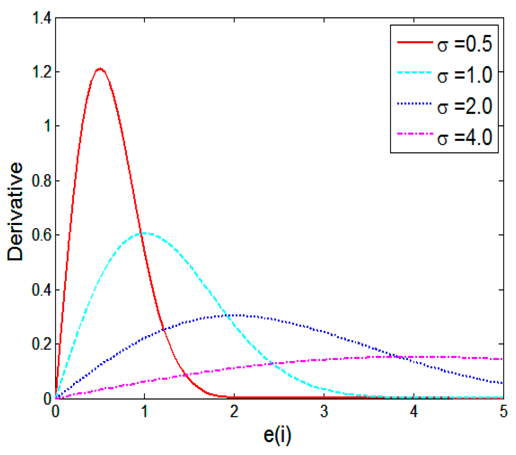
Figure 1 shows the structure of a Hammerstein adaptive filter under MCC criterion, where the filter consists of a polynomial memoryless nonlinearity followed by a linear FIR filter. This structure has been commonly used in Hammerstein adaptive filtering [8,9,27]. As shown in Figure 1, under the MCC criterion, the parameters of the linear and nonlinear parts are adjusted to maximize the correntropy between the model output and desired response.
Figure 1. Structure of a Hammerstein adaptive filter under maximum correntropy criterion (MCC) criterion.
Entropy 17 07149 g001

2.1. Correntropy

Correntropy is a nonlinear similarity measure between two signals. Given two random variables X and Y, the correntropy is [33,34,35,36,37,38,39]
V ( X , Y ) = E [ κ ( X , Y ) ] = κ ( x , y ) f X Y ( x , y ) d x d y
where E[·] denotes the expectation operator, κ(·,·) is a shift-invariant Mercer kernel, and fXY(x, y) stands for the probability density function (PDF) of (X, Y). The most widely used kernel in correntropy is the Gaussian kernel, given by
κ σ ( x , y ) = 1 σ 2 π exp ( e 2 2 σ 2 )
where e = xy, and σ stands for the kernel bandwidth. In this work, without being mentioned otherwise, the kernel function is a Gaussian kernel. In practical situations, the join distribution of X and Y is usually unknown and only a finite number of data {(d(i), y(i))} i = 1 K are available. In these cases, one can use a sample mean estimator of the correntropy:
V ^ N , σ ( X , Y ) = 1 K i = 1 K κ σ ( d ( i ) y ( i ) )
The optimization cost under MCC is thus
max J M C C = i = 1 K κ σ ( e ( i ) )
where e(i) = d(i) − y(i). We can evaluate the sensitivity (derivative) of the MCC cost JMCC with respect to the error e(i),
J M C C e ( i ) = 1 2 π σ 3 exp ( e 2 ( i ) 2 σ 2 ) e ( i )
The derivative curves of −JMCC for different kernel widths are illustrated in Figure 2. As one can see, when the magnitude of error is very large, the derivative will become rather small especially for a smaller kernel width. Therefore, the MCC training is insensitive (hence robust) to a large error.
Figure 2. Derivative curves of −JMCC with respect to e(i) for different kernel widths.
Entropy 17 07149 g002

2.2. Hammerstein Adaptive Filtering

Assuming that the input-output mapping of the memoryless polynomial nonlinearity is
s ( n ) = p 1 x ( n ) + p 2 x 2 ( n ) + + p M x M ( n )
where M and pM denote the polynomial order and the m-th order coefficient, Expression (6) can be rewritten as
s ( n ) = p T ( n ) x p ( n )
where xp(n) = [x(n) x2(n)···xM(n)]T is the polynomial regressor, and p(n) = [p1 p2···pM]T is the polynomial coefficient vector. The output of the FIR filter can be expressed as
y ( n ) = w T ( n ) s ( n )
where w(n) = [w0 w1···wN−1]T is the FIR weight vector, and s(n) = [s(n) s(n − 1)···s(nN + 1)]T is the FIR input vector, with N being the FIR memory size. Let X(n) = [xp(n) xp(n − 1)···xp(nN + 1)]T. Then we have
s ( n ) = Χ T ( n ) p ( n )
Combining Equations (8) and (9) yields
y ( n ) = w T ( n ) s ( n ) = w T ( n ) Χ T ( n ) p ( n )
Assume that the unknown system that needs to be identified is also a Hammerstein system with parameter vectors p * = [ p 1 *   p 2 * · · · p M * ] T and w * = [ w 0 *   w 1 * · · · w N 1 * ] T . Then, the desired signal can be expressed as
d ( n ) = w * T Χ T ( n ) p + v ( n )
where v(n) stands for an additive disturbance noise. The error signal can then be calculated as e(n) = d(n) − wT(n)XT(n)p(n). In the following, we derive an adaptive algorithm to estimate the Hammerstein parameter vectors using MCC instead of MSE as an optimization criterion. Let us consider the following cost function
J M C C ( p,w ) = j = n L + 1 n κ σ ( d ( j ) , y ( j ) )                   = 1 2 π σ j = n L + 1 n exp ( e 2 ( j ) 2 σ 2 )
where e(j) = d(j) − y(j), and L denotes the sliding data length. Then, a steepest ascent algorithm for estimating the polynomial coefficient vector can be derived as follows:
J M C C ( p,w ) p ( n ) = 1 2 π σ 3 j = n L + 1 n exp ( e 2 ( j ) 2 σ 2 ) e ( j ) e ( j ) p ( j )                     = 1 2 π σ 3 j = n L + 1 n exp ( e 2 ( j ) 2 σ 2 ) e ( j ) Χ ( j ) w ( j )
p ( n + 1 ) = p ( n ) + μ p J M C C ( p,w ) p ( n ) = p ( n ) + μ p 2 π σ 3 j = n L + 1 n exp ( e 2 ( j ) 2 σ 2 ) e ( j ) Χ ( j ) w ( j )
In a similar way, we propose the following weight update equation for the coefficients of the FIR filter:
J M C C ( p,w ) w ( n ) = 1 2 π σ 3 j = n L + 1 n exp ( e 2 ( j ) 2 σ 2 ) e ( j ) e ( j ) w ( j )                     = 1 2 π σ 3 j = n L + 1 n exp ( e 2 ( j ) 2 σ 2 ) e ( j ) Χ T ( j ) p ( j )
w ( n + 1 ) = w ( n ) + μ w J M C C ( p,w ) w ( n ) = w ( n ) + μ w 2 π σ 3 j = n L + 1 n exp ( e 2 ( j ) 2 σ 2 ) e ( j ) Χ T ( j ) p ( j )
In Equations (14) and (16), μp and μw are, respectively, step-sizes for polynomial nonlinearity subsystem and FIR subsystem. In this work, for simplicity we consider only the stochastic gradient based algorithm (i.e., L = 1). In this case, we have
p ( n + 1 ) = p ( n ) + η p exp ( e 2 ( n ) 2 σ 2 ) e ( n ) Χ ( n ) w ( n )
w ( n + 1 ) = w ( n ) + η w exp ( e 2 ( n ) 2 σ 2 ) e ( n ) Χ T ( n ) p ( n )
where η p = μ p 2 π σ 3 , and η w = μ w 2 π σ 3 . The above update equations are referred to as the Hammerstein adaptive filtering algorithm under MCC criterion, whose pseudocodes are presented in Algorithm 1. The proposed algorithm is in form similar to the traditional Hammerstein adaptive filters under MSE criterion [7], but the step-sizes are different.
Algorithm 1: Hammerstein adaptive filtering Algorithm under MCC.
Parameters setting: μp, μw, σ
Initialization: p(0), w(0)
For n = 1, 2, … do
(1)
s ( n ) = Χ T ( n ) p ( n )
(2)
y ( n ) = w T ( n ) s ( n )
(3)
e ( n ) = d ( n ) y ( n )
(4)
p ( n + 1 ) = p ( n ) + η p exp ( e 2 ( n ) 2 σ 2 ) e ( n ) Χ ( n ) w ( n )
(5)
w ( n + 1 ) = w ( n ) + η w exp ( e 2 ( n ) 2 σ 2 ) e ( n ) Χ T ( n ) p ( n )
End for

3. Convergence Analysis

3.1. Stability Analysis

Using the Taylor series expansion of the error e(n + 1) around the instant n and keeping only the linear term, we have [4,7,40]
e ( n + 1 ) = e ( n ) + e ( n ) p ( n ) | w ( n ) = c o n s t Δ p ( n ) + e ( n ) w ( n ) | p ( n ) = c o n s t Δ w ( n ) + h . o . t
where h.o.t denotes higher-order terms. Combining Equations (11), (17) and (18), we can obtain
e ( n ) p ( n ) = Χ ( n ) w ( n )
e ( n ) w ( n ) = Χ T ( n ) p ( n )
Δ p ( n ) = η p exp ( e 2 ( n ) 2 σ 2 ) e ( n ) Χ ( n ) w ( n )
Δ w ( n ) = η w exp ( e 2 ( n ) 2 σ 2 ) e ( n ) Χ T ( n ) p ( n )
Substituting Equations (20)–(23) in Equation (19), and after simple manipulation, we have
e ( n + 1 ) = [ 1 η p exp ( e 2 ( n ) 2 σ 2 ) Χ ( n ) w ( n ) 2 η w exp ( e 2 ( n ) 2 σ 2 ) Χ T ( n ) p ( n ) 2 ] e ( n )
To ensure the stability of the proposed algorithm, we must assure that |e(n + 1)| ≤ |e(n)|, and hence
| 1 η p exp ( e 2 ( n ) 2 σ 2 ) Χ ( n ) w ( n ) 2 η w exp ( e 2 ( n ) 2 σ 2 ) Χ T ( n ) p ( n ) 2 | 1
which yields
0 < η p Χ ( n ) w ( n ) 2 + η w Χ T ( n ) p ( n ) 2 2 exp ( e 2 ( n ) 2 σ 2 )
Since exp ( e 2 ( n ) 2 σ 2 ) 1 , the following condition guarantees convergence:
0 < η p Χ ( n ) w ( n ) 2 + η w Χ T ( n ) p ( n ) 2 2
Remark 1. The derived bound on step-sizes is only of theoretical importance as in general, Equation (27) cannot be verified in a practical situation. Similar theoretical results can be found in [7].

3.2. Steady-State Mean Square Performance

We denote epw(n) the a priori error of the whole system, ep(n) the a priori error when only the nonlinear part is adapted while the linear filter is fixed, and ew(n) the a priori error when only the linear filter is adapted while the nonlinear part is fixed. Let Η p = lim n E [ e p 2 ( n ) ] , Η w = lim n E [ e w 2 ( n ) ] , and Η p w = lim n E [ e p w 2 ( n ) ] be the steady-state excess mean square errors (EMSEs). In addition, we denote
f ( e ( i ) ) = exp ( e 2 ( i ) 2 σ 2 ) e ( i )
Before evaluating the theoretical values of the steady-state EMSEs, we make the following assumptions:
(A)
The noise v(n) is zero-mean, independent, identically distributed, and is independent of the input X(n), s ^ ( n ) and e(n).
(B)
The a priori errors ep(n) and ew(n) are zero-mean Gaussian, and independent of the noise v(n).
(C)
||X(n)w(n)||2 and ||XT(n)p(n)||2 are asymptotically uncorrelated with f2(e(n)), that is
lim n E [ Χ ( n ) w ( n ) 2 f 2 ( e ( n ) ) ] = T r ( R W X ) lim n E [ f 2 ( e ( n ) ) ]
lim n E [ Χ T ( n ) p ( n ) 2 f 2 ( e ( n ) ) ] = T r ( R X P ) lim n E [ f 2 ( e ( n ) ) ]
where R W X = E [ ( Χ ( n ) w ( n ) ) ( Χ ( n ) w ( n ) ) T ] and R X P = E [ ( Χ T ( n ) p ( n ) ) ( Χ T ( n ) p ( n ) ) T ] are the covariance matrices, and T r ( ) denotes the trace operator.
Remark 2. For the assumption (A), it is very common to assume that the noise is independent of the regression vector [41,42,43]. In addition, the noise is often restricted to be zero-mean, identically distributed [33,34,35]. As discussed in [44,45], the assumption (B) is reasonable for long adaptive filters. Since ep(n) is the a priori error when only the nonlinear part is adapted while the linear filter is fixed, we have the approximation w*w(n) such that w(n) is asymptotically uncorrelated with f2(e(n)). Due to the independent assumption (A), X(n) is also asymptotically uncorrelated with f2(e(n)). So ||XT(n)w(n)||2 is asymptotically uncorrelated with f2(e(n)). Similarly, ||XT(n)p(n)||2 is asymptotically uncorrelated with f2(e(n)). Therefore, the assumption (C) is rational.
When only the polynomial part with parameter vector p is adapted, the error ep(n) is
e p ( n ) = w * T Χ T ( n ) p w T ( n ) Χ T ( n ) p ( n ) w T ( n ) Χ T ( n ) p ˜ ( n )
where p ˜ ( n ) = p * p T ( n ) . In Equation (31), we use the approximation w*w(n) at steady-state. From Equation (17), it follows easily that
p ˜ ( n + 1 ) = p ˜ ( n ) η p f ( e ( n ) ) Χ ( n ) w ( n )
Squaring both sides of Equation (32), we have
p ˜ ( n + 1 ) 2 = p ˜ ( n ) 2 2 η p f ( e ( n ) ) e p ( n ) + η p 2 f 2 ( e ( n ) ) Χ ( n ) w ( n ) 2
Taking the expectations of the both sides of Equation (33) yields
E [ p ˜ ( n + 1 ) 2 ] = E [ p ˜ ( n ) 2 ] 2 η p E [ f ( e ( n ) ) e p ( n ) ] + η p 2 E [ f 2 ( e ( n ) ) Χ ( n ) w ( n ) 2 ]
Assuming the filter is stable and attains the steady state, it holds
lim n E [ p ˜ ( n + 1 ) 2 ] = lim n E [ p ˜ ( n ) 2 ]
Combining Equations (34) and (35) and the above assumptions, we obtain
2 lim n E [ f ( e ( n ) ) e p ( n ) ] = η p T r ( R W X ) lim n E [ f 2 ( e ( n ) ) ]
In order to derive a theoretical value of the steady-state EMSE, we consider two cases below.
Case A. Gaussian Noise
Recalling that e(n) = ep(n) + v(n), and assuming that the noise v(n) is zero-mean Gaussian, with variance ϛ v 2 , we get [34]
lim n E [ f ( e ( n ) ) e p ( n ) ] = σ 3 Η p ( σ 2 + ς v 2 + Η p ) 3 / 2
where σ e 2 denotes the variance of the error, and σ e 2 = E[ e p 2 (n)] + ϛ v 2 . Similarly, we obtain [29]
lim n E [ f 2 ( e ( n ) ) ] = σ 3 ( Η p + ς v 2 ) ( σ 2 + 2 ς v 2 + 2 Η p ) 3 / 2
Substituting Equations (37) and (38) into Equation (36), we have
2 σ 3 Η p ( σ 2 + ς v 2 + Η p ) 3 / 2 = η p T r ( R W X ) σ 3 ( Η p + ς v 2 ) ( σ 2 + 2 ς v 2 + 2 Η p ) 3 / 2
Therefore, the steady-state EMSE Hp satisfies
Η p = η p 2 T r ( R W X ) ( Η p + ς v 2 ) ( σ 2 + ς v 2 + Η p ) 3 / 2 ( σ 2 + 2 ς v 2 + 2 Η p ) 3 / 2
Theorem 1. In a Gaussian noise environment and with the same step-size, the proposed nonlinear Hammerstein adaptive filter under MCC criterion has a smaller steady-state EMSE than under MSE criterion. As the kernel width increases, their values of the steady-state EMSE will become almost identical.
Proof. It can be shown that [34]
Η p M S E = η p T r ( R W X ) ς v 2 2 η p T r ( R W X )
where HpMSE denotes the steady-state EMSE under MSE criterion. From Equation (40), we have
Η p = ε η p T r ( R W X ) ς v 2 2 ε η p T r ( R W X )
where ε = ( σ 2 + ς v 2 + Η p ) 3 / 2 ( σ 2 + 2 ς v 2 + 2 Η p ) 3 / 2 . Since ε < 1 , it holds
Η p < Η p M S E
Further, as σ → ∞, we have Hp → HpMSE.
Case B. Non-Gaussian Noise
Taking the Taylor series expansion of f(e(n)) around v(n) yields
f ( e ( n ) ) = f ( e p ( n ) + v ( n ) )              = f ( v ( n ) ) + f ( v ( n ) ) e p ( n ) + 1 2 f ( v ( n ) ) e p 2 ( n ) + h . o . t
with
f ( v ( n ) ) = exp ( v 2 ( n ) 2 σ 2 ) ( 1 v 2 ( n ) σ 2 ) f ( v ( n ) ) = exp ( v 2 ( n ) 2 σ 2 ) ( v 3 ( n ) σ 4 3 v ( n ) σ 2 )
Under the assumptions (A) and (B), we get [34]
lim n E [ f ( e ( n ) ) e p ( n ) ] E [ f ( v ( n ) ) ] Η p
lim n E [ f 2 ( e ( n ) ) ] E [ f 2 ( v ( n ) ) ] + E [ f ( v ( n ) ) f ( v ( n ) ) + | f ( v ( n ) ) | 2 ] Η p
Substituting Equations (46) and (47) into Equation (36), we have
Η p = η p T r ( R W X ) E [ f 2 ( v ( n ) ) ] 2 E [ f ( v ( n ) ) ] η p T r ( R W X ) E [ f ( v ( n ) ) f ( v ( n ) ) + | f ( v ( n ) ) | 2 ]
Further, substituting Equation (45) into Equation (48), we obtain
Η p = η p T r ( R W X ) E [ exp ( v 2 ( n ) σ 2 ) v 2 ( n ) ] 2 E [ exp ( v 2 ( n ) 2 σ 2 ) ( 1 v 2 ( n ) σ 2 ) ] η p T r ( R W X ) E [ exp ( v 2 ( n ) σ 2 ) ( 1 + 2 v 4 ( n ) σ 4 5 v 2 ( n ) σ 2 ) ]
When only the linear filter with parameter vector w(n) is adapted, we get
2 lim n E [ f ( e ( n ) ) e w ( n ) ] = η p T r ( R X P ) lim n E [ f 2 ( e ( n ) ) ]
where e w ( n ) w ˜ T ( n ) Χ T ( n ) p ( n ) , w ˜ ( n ) = w * w ( n ) . For Gaussian noise case, we obtain
Η w = η w 2 T r ( R X P ) ( Η w + ς v 2 ) ( σ 2 + ς v 2 + Η w ) 3 / 2 ( σ 2 + 2 ς v 2 + 2 Η w ) 3 / 2
In non-Gaussian environments, we have
Η w = η w T r ( R X P ) E [ exp ( v 2 ( n ) σ 2 ) v 2 ( n ) ] 2 E [ exp ( v 2 ( n ) 2 σ 2 ) ( 1 v 2 ( n ) σ 2 ) ] η w T r ( R X P ) E [ exp ( v 2 ( n ) σ 2 ) ( 1 + 2 v 4 ( n ) σ 4 5 v 2 ( n ) σ 2 ) ]
Theorem 2. The Hpw satisfies the following condition
Η p w Η p + Η w
Proof. Using Equation (31), we derive
e p w ( n ) = w * T Χ T ( n ) p w T ( n ) Χ T ( n ) p ( n )           = ( w * T Χ T ( n ) p w * T ( n ) Χ T ( n ) p ( n ) ) + ( w * T Χ T ( n ) p ( n ) w T ( n ) Χ T ( n ) p ( n ) )           w T ( n ) Χ T ( n ) p ˜ ( n ) w ˜ T ( n ) Χ T ( n ) p ( n )           = e p ( n ) + e w ( n )
It follows that
Η p w = lim n E [ e 2 p w ( n ) ] lim n E [ ( e p ( n ) + e w ( n ) ) 2 ]        = lim n E [ e p 2 ( n ) ] + 2 lim n E [ e p ( n ) e w ( n ) ] + lim n E [ e w 2 ( n ) ]        = Η p + Η w + 2 Η c r o s s
where Η c r o s s = lim n E [ e p ( n ) e w ( n ) ] stands for the cross-EMSE and Hcross ≥ 0 (Hcross = 0 when ep(n) and ew(n) are statistically independent and zero mean) [7]. Therefore, Hpw ≥ Hp + Hw, which completes the proof.

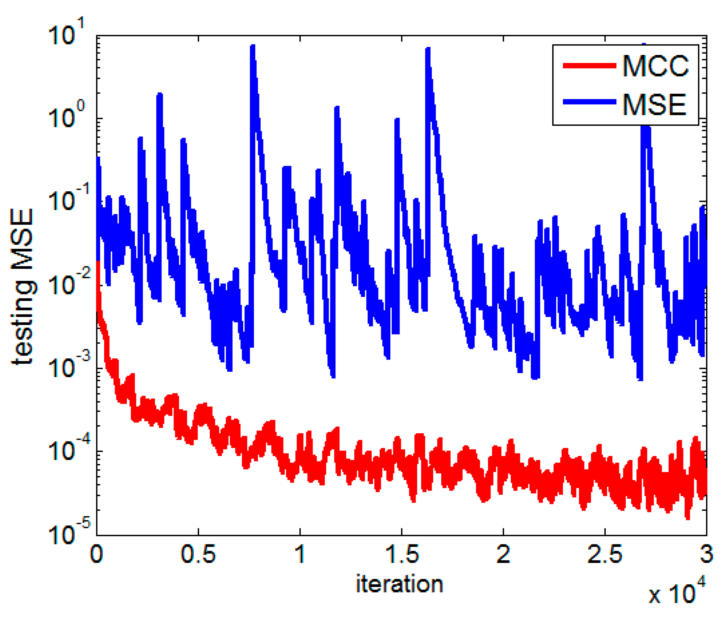
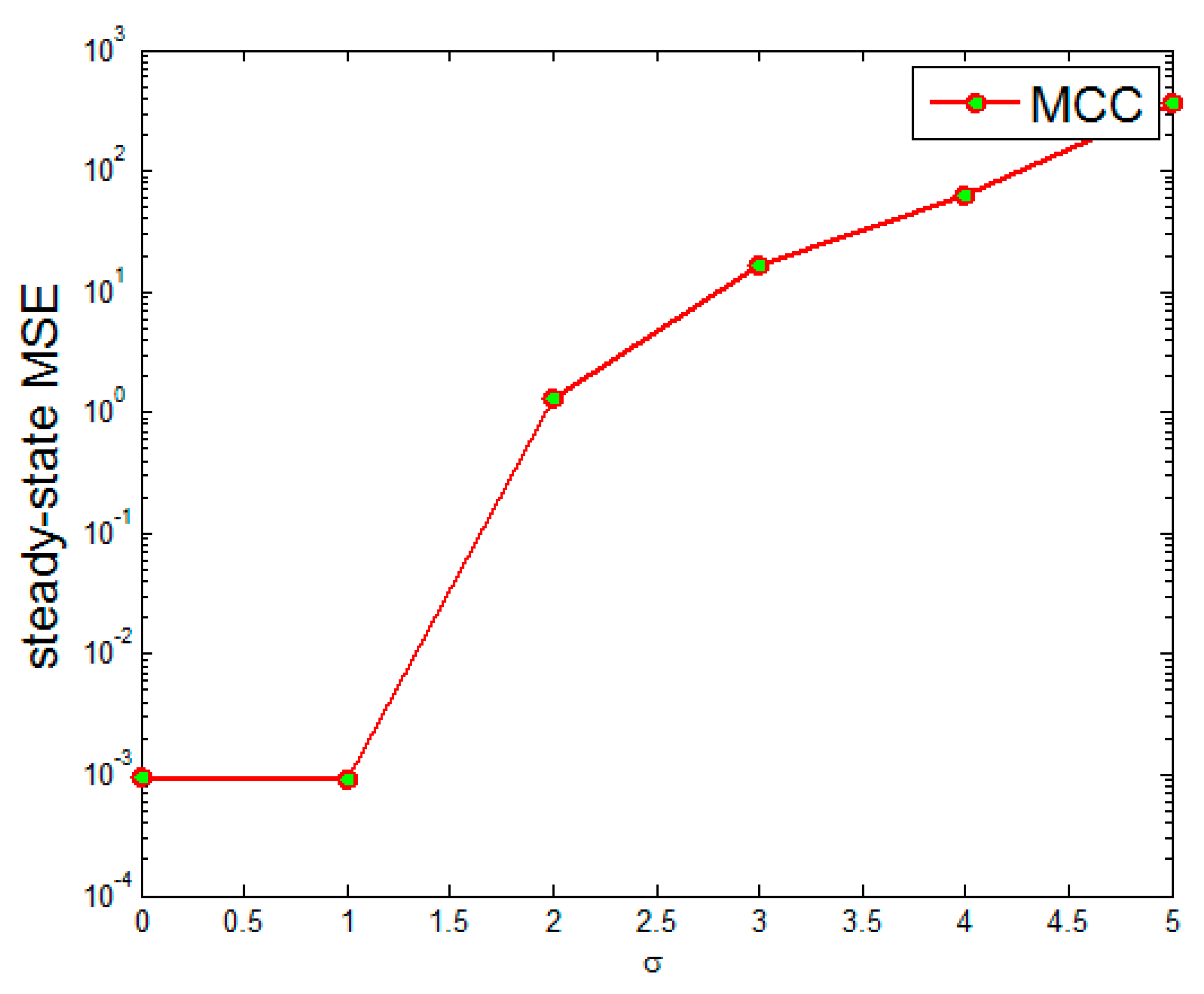
4. Simulation Results
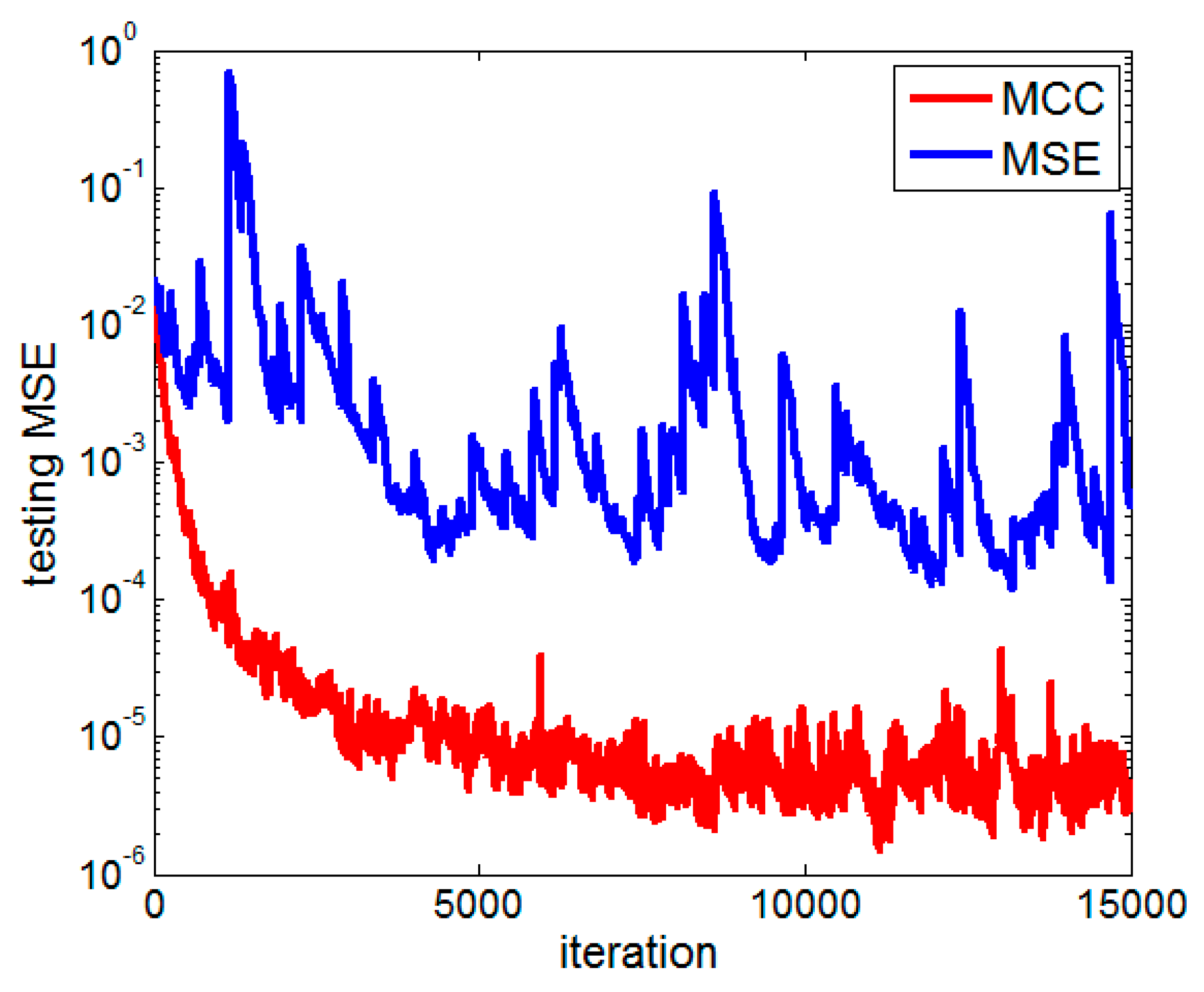
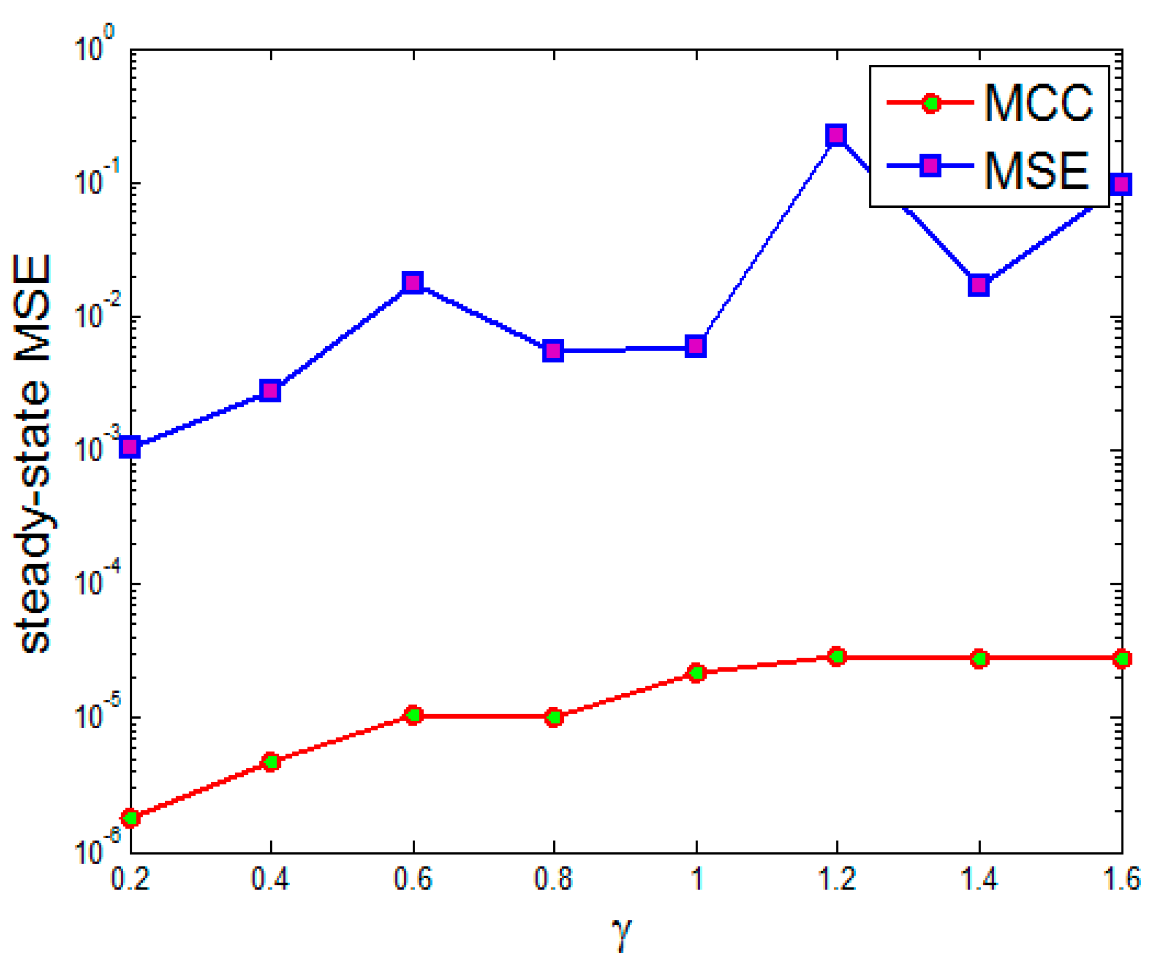
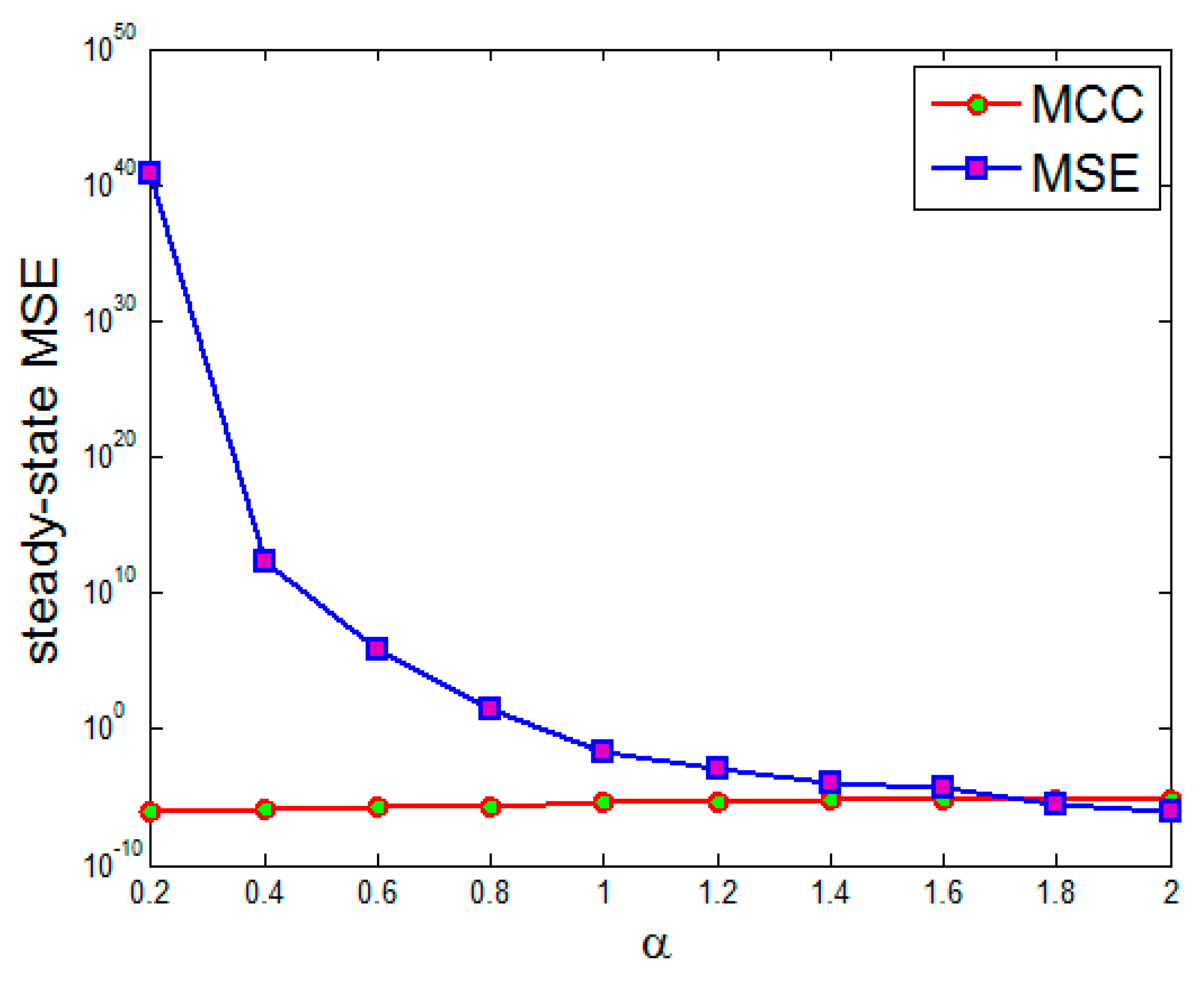
Now, we present simulation results to demonstrate the performance of the Hammerstein adaptive filtering under MCC. In order to show the performance of the proposed algorithm in non-Gaussian noises, we adopt the alpha-stable distribution to generate the disturbance noise, whose characteristic function is [32,46]
f ( t ) = exp { j δ t γ | t | α [ 1 + j β sgn ( t ) S ( t , α ) ] }
in which
S ( t , α ) = { tan α π 2 i f   α 1 2 π log | t | i f   α = 1
where α ϵ (0, 2] denotes the characteristic factor, −∞ < δ < +∞ is the location parameter, β ϵ [−1, 1] stands for the symmetry parameter, and γ > 0 is the dispersion parameter. The characteristic factor α measures the tail heaviness of the distribution. The smaller α is, the heavier the tail is. In addition, γ measures the dispersion of the distribution. The distribution is symmetric about its location δ when β = 0. Such a distribution is called a symmetric alpha-stable (SαS) distribution. The parameters vector of the noise model is defined as V = (α, β, γ, δ).
In the simulations below, the input signal considered is a colored signal obtained from the following equation:
x ( n ) = a x ( n 1 ) + 1 a 2 ξ ( n )
with a = 0.95, and ξ(n) being a white Gaussian signal of unit variance. In addition, the coefficient vectors are initialized with the first coefficient equal to 1 and the others equal to zero [7].

4.1. Experiment 1

First, we consider an unknown Hammerstein system with parameter vectors p* = [1, 0.6], w* = [1, 0.6, 0.1, −0.2, −0.06, 0.04, 0.02, −0.03, −0.02, 0.01]. Thus, M = 2, N = 10. The kernel width σ is 1.0. The noise vector V is set at (1.2, 0, 0.6, 0), and the noise signal is shown in Figure 3. Simulation results are averaged over 100 independent Monte Carlo runs, and in each simulation, 15,000 iterations are run to ensure the algorithm will reach the steady state, and the steady-state MSE is obtained as an average over the last 2000 iterations. The step-sizes are set at μp = μw = 0.005 and μp = 0.01, μw = 0.01 for MSE and MCC, respectively. Figure 4 shows the average convergence curves under MCC and MSE. As we can see, the Hammerstein adaptive filtering under MCC criterion achieves faster convergence speed and lower steady-state testing MSE than under MSE criterion. Here the testing MSE is evaluated on a test set with 100 samples.
Figure 3. A typical sequence of the alpha-stable noise with V = (1.2, 0, 0.6, 0).
Entropy 17 07149 g003
Figure 4. Convergence curves under maximum correntropy criterion (MCC) and mean square error (MSE) (for unknown system with polynomial nonlinearity).
Entropy 17 07149 g004
Second, we investigate the performance of the algorithms with different noise parameters. The steady-state MSEs with different γ (0.2, 0.4, 0.6, 0.8, 1.0, 1.2, 1.4, 1.6) and different α (0.2, 0.4, 0.6, 0.8, 1, 1.2, 1.4, 1.6, 1.8, 2.0) are shown in Figure 5 and Figure 6, respectively. We observe: (1) In most cases, the new algorithm performs better and achieves a lower steady-state MSE compared with the Hammerstein adaptive filtering under MSE criterion; (2) When α is close to 2.0, the Hammerstein adaptive filtering under MSE criterion can achieve better performance than under MCC criterion. The main reason for this is that, when α ≈ 2.0, the noise will be approximately Gaussian. Simulation results suggest that the proposed algorithm is particularly useful for identifying a Hammerstein system in non-Gaussian noises.
Figure 5. Steady-state mean square error (MSE) with different γ (α = 1.2).
Entropy 17 07149 g005
Figure 6. Steady-state mean square error (MSE) with different α (γ = 0.6).
Entropy 17 07149 g006

4.2. Experiment 2

The second experiment is drawn from [47]. The nonlinear dynamic system is composed of two blocks. The first block is a non-polynomial nonlinearity
s ( n ) = x ( n ) 3
while the second block is an FIR filter with weight vector
h = [ 1   0.75   0.5   0.25   0   0.25 ] T
The noise vector V is set at (1.0, 0, 0.8, 0) (see Figure 7 for a typical sequence of the noise), and the polynomial order M and the FIR memory size N are set at 3 and 6, respectively. Simulation results are averaged over 50 independent Monte Carlo runs, and in each simulation, 30,000 iterations are run to ensure the algorithm will reach the steady state, and the steady-state MSE is obtained as an average over the last 2000 iterations. The testing MSE is evaluated on a test set with 100 samples. Figure 8 demonstrates the convergence curves under MCC and MSE. For both adaptive filtering algorithms, the step-sizes are set at μp = 0.005, μw = 0.015. It can be seen that, the Hammerstein adaptive filter under MCC criterion performs better (say, with faster convergence speed and smaller mismatch error) than under MSE criterion.
Figure 7. A typical sequence of the alpha-stable noise with V = (1.0, 0, 0.8, 0).
Entropy 17 07149 g007
Figure 8. Convergence curves under maximum correntropy criterion (MCC) and mean square error (MSE) (for unknown system with non-polynomial nonlinearity).
Entropy 17 07149 g008
Finally, we show the steady-state performance of the algorithms with different kernel widths σ (0.01, 1.0, 2.0, 3.0, 4.0, 5.0). Simulation results are shown in Figure 9. As we can see, the kernel width has significant influence on the performance of the proposed algorithm. In this example, the lowest steady-state MSE is obtained when σ = 1.0.
Figure 9. Steady-state mean square error (MSE) with different kernel widths.
Entropy 17 07149 g009

5. Conclusions

The MCC has been successfully applied in domains of machine learning and signal processing due to its strong robustness in impulsive non-Gaussian situations. In this work, we develop a robust Hammerstein adaptive filter under MCC criterion. Different from the traditional Hammerstein adaptive filtering algorithms, the new algorithm use the MCC instead of the well-known MSE as the adaptation criterion, which can achieve desirable performance especially in impulsive noises. Based on [7,31], we carry out the convergence analysis, and obtain some important theoretical results. Simulation examples confirm the excellent performance of the proposed algorithm. How to verify the derived theoretical results is an interesting topic for future study.

Acknowledgments

This work was supported by 973 Program (No. 2015CB351703) and National Natural Science Foundation of China (No. 61372152, No. 61271210).

Author Contributions

Zongze Wu derived the algorithm and wrote the draft; Siyuan Peng proved the convergence properties and performed the simulations; Badong Chen proposed the main idea and polished the language; Haiquan Zhao was in charge of technical checking. All authors have read and approved the final manuscript.

Conflicts of Interest

The authors declare no conflict of interest.

References

  1. Ljung, L. System Identification—Theory for the User, 2nd ed.; Prentice Hall: Upper Saddle River, NJ, USA, 1999. [Google Scholar]
  2. Sayed, A.H. Fundamentals of Adaptive Filtering; Wiley: Hoboken, NJ, USA, 2003. [Google Scholar]
  3. Wiener, N. Nonlinear Problems in Random Theory; MIT Press: Cambridge, MA, USA, 1958. [Google Scholar]
  4. Scarpiniti, M.; Comminiello, D.; Parisi, R.; Uncini, A. Nonlinear spline adaptive filtering. Signal Process. 2013, 93, 772–783. [Google Scholar] [CrossRef]
  5. Bai, E.W. Frequency domain identification of Wiener models. Automatica 2003, 39, 1521–1530. [Google Scholar] [CrossRef]
  6. Ogunfunmi, T. Adaptive Nonlinear System Identification: The Volterra and Wiener Model Approaches; Springer: Berlin/Heidelberg, Germany, 2007. [Google Scholar]
  7. Scarpiniti, M.; Comminiello, D.; Parisi, R.; Uncini, A. Hammerstein uniform cubic spline adaptive filters: Learning and convergence properties. Signal Process. 2014, 100, 112–123. [Google Scholar] [CrossRef]
  8. Ortiz Batista, E.L.; Seara, R. A new perspective on the convergence and stability of NLMS Hammerstein filters. In Proceedings of the IEEE 8th International Symposium on Image and Signal Processing and Analysis (ISPA), Trieste, Italy, 4–6 September 2013; pp. 343–348.
  9. Bai, E.W.; Li, D. Convergence of the iterative Hammerstein system identification algorithm. IEEE Trans. Autom. Control 2004, 49, 1929–1940. [Google Scholar] [CrossRef]
  10. Umoh, I.; Ogunfunmi, T. An Affine-Projection-Based Algorithm for Identification of Nonlinear Hammerstein Systems. Signal Process. 2010, 90, 2020–2030. [Google Scholar] [CrossRef]
  11. Umoh, I.; Ogunfunmi, T. An Adaptive Nonlinear Filter for System Identification. EURASIP J. Adv. Signal Process. 2009, 2009. [Google Scholar] [CrossRef]
  12. Umoh, I.; Ogunfunmi, T. An adaptive algorithm for Hammerstein filter system identification. In Proceedings of the EURASIP European Signal Processing Conference, Lausanne, Switzerland, 25–29 August 2008; pp. 1–5.
  13. Greblicki, W. Continuous time Hammerstein system identification. IEEE Trans. Autom. Control 2000, 45, 1232–1236. [Google Scholar] [CrossRef]
  14. Jeraj, J.; Mathews, V.J. Stochastic mean-square performance analysis of an adaptive Hammerstein filter. IEEE Trans. Signal Process. 2006, 54, 2168–2177. [Google Scholar] [CrossRef]
  15. Voros, J. Iterative algorithm for parameter identification of Hammerstein systems with two-segment nonlinearities. IEEE Trans. Autom. Control 1999, 44, 2145–2149. [Google Scholar] [CrossRef]
  16. Greblicki, W. Stochastic approximation in nonparametric identification of Hammerstein systems. IEEE Trans. Autom. Control 2002, 47, 1800–1810. [Google Scholar] [CrossRef]
  17. Ding, F.; Liu, X.P.; Liu, G. Identification methods for Hammerstein nonlinear systems. Dig. Signal Process. 2011, 21, 215–238. [Google Scholar] [CrossRef]
  18. Jeraj, J.; Matthews, V.J. A stable adaptive Hammerstein filter employing partial orthogonalization of the input signals. IEEE Trans. Signal Process. 2006, 54, 1412–1420. [Google Scholar] [CrossRef]
  19. Nordsjo, A.E.; Zetterberg, L.H. Identification of certain time-varying nonlinear Wiener and Hammerstein systems. IEEE Trans. Signal Process. 2001, 49, 577–592. [Google Scholar] [CrossRef]
  20. Atiya, A.; Parlos, A. Nonlinear system identification using spatiotemporal neural networks. In Proceedings of the International Joint Conference on Neural Networks, Baltimore, MD, USA, 7–11 June 1992; pp. 504–509.
  21. Volterra, V. Theory of Functionals and of Integral and Integro-Differential Equations; Courier Corporation: North Chelmsford, MA, USA, 2005. [Google Scholar]
  22. Principe, J.C.; Liu, W.; Haykin, S. Kernel Adaptive Filtering: A Comprehensive Introduction; Wiley: Hoboken, NJ, USA, 2011. [Google Scholar]
  23. Chen, B.; Zhao, S.; Zhu, P.; Principe, J.C. Quantized kernel least mean square algorithm. IEEE Trans. Neural Netw. Learn. Syst. 2012, 23, 22–32. [Google Scholar] [CrossRef] [PubMed]
  24. Chen, B.; Zhao, S.; Zhu, P.; Principe, J.C. Quantized kernel recursive least squares algorithm. IEEE Trans. Neural Netw. Learn. Syst. 2013, 24, 1484–1491. [Google Scholar] [CrossRef] [PubMed]
  25. Chen, B.; Zhao, S.; Zhu, P.; Principe, J.C. Mean square convergence analysis of the kernel least mean square algorithm. Signal Process. 2012, 92, 2624–2632. [Google Scholar] [CrossRef]
  26. Bai, E.W. A blind approach to Hammerstein model identification. IEEE Trans. Signal Process. 2002, 50, 1610–1619. [Google Scholar] [CrossRef]
  27. Stenger, A.; Kellermann, W. Adaptation of a memoryless preprocessor for nonlinear acoustic echo cancelling. Signal Process. 2000, 80, 1747–1760. [Google Scholar] [CrossRef]
  28. Shi, K.; Ma, X.; Zhou, G.T. An efficient acoustic echo cancellation design for systems with long room impulses and nonlinear loudspeakers. Signal Process. 2009, 89, 121–132. [Google Scholar] [CrossRef]
  29. Scarpiniti, M.; Comminiello, D.; Parisi, R.; Uncini, A. Comparison of Hammerstein and Wiener systems for nonlinear acoustic echo cancelers in reverberant environments. In Proceedings of the 17th International Conference on Digital Signal Processing (DSP), Corfu, Greece, 6–8 July 2011; pp. 1–6.
  30. Kailath, T.; Sayed, A.H.; Hassibi, B. Linear Estimation; Prentice Hall: Upper Saddle River, NJ, USA, 2000. [Google Scholar]
  31. Plataniotis, K.N.; Androutsos, D.; Venetsanopoulos, A.N. Nonlinear filtering of non-Gaussian noise. J. Intell. Robot. Syst. 1997, 19, 207–231. [Google Scholar] [CrossRef]
  32. Weng, B.; Barner, K.E. Nonlinear system identification in impulsive environments. IEEE Trans. Signal Process. 2005, 53, 2588–2594. [Google Scholar] [CrossRef]
  33. Chen, B.; Zhu, Y.; Hu, J.; Principe, J.C. System Parameter Identification: Information Criteria and Algorithms; Elsevier: Amsterdam, The Netherlands, 2013. [Google Scholar]
  34. Chen, B.; Xing, L.; Liang, J.; Zheng, N.; Principe, J.C. Steady-state Mean-square Error Analysis for Adaptive Filtering under the Maximum Correntropy Criterion. IEEE Signal Process. Lett. 2014, 21, 880–884. [Google Scholar]
  35. Principe, J.C. Information Theoretic Learning: Renyi’s Entropy and Kernel Perspectives; Springer: New York, NY, USA, 2010. [Google Scholar]
  36. Singh, A.; Principe, J.C. Using Correntropy as a cost function in linear adaptive filters. In Proceedings of the IEEE International Joint Conference on Neural Networks (IJCNN), Atlanta, GA, USA, 14–19 June 2009; pp. 2950–2955.
  37. Chen, B.; Principe, J.C. Maximum correntropy estimation is a smoothed MAP estimation. IEEE Signal Process. Lett. 2012, 19, 491–494. [Google Scholar] [CrossRef]
  38. Zhao, S.; Chen, B.; Principe, J.C. Kernel adaptive filtering with maximum correntropy criterion. In Proceedings of the IEEE International Joint Conference on Neural Networks (IJCNN), Killarney, Ireland, 31 July–5 August 2011; pp. 2012–2017.
  39. Ogunfunmi, T.; Paul, T. The Quaternion Maximum Correntropy Algorithm. IEEE Trans. Circuits Syst. -II (TCAS-II) 2015, 62, 598–602. [Google Scholar] [CrossRef]
  40. Mandic, D.P.; Hanna, A.I.; Razaz, M. A normalized gradient descent algorithm for nonlinear adaptive filters using a gradient adaptive step size. IEEE Signal Process. Lett. 2001, 8, 295–297. [Google Scholar] [CrossRef]
  41. Al-Naffouri, T.Y.; Sayed, A.H. Adaptive filters with error non-linearities: Mean-square analysis and optimum design. EURASIP J. Appl. Signal Process. 2001, 4, 192–205. [Google Scholar] [CrossRef]
  42. Lin, B.; He, R.; Wang, X.; Wang, B. The steady-state mean-square error analysis for least mean p-order algorithm. IEEE Signal Process. Lett. 2009, 16, 176–179. [Google Scholar] [CrossRef]
  43. Yousef, N.R.; Sayed, A.H. A unified approach to the steady-state and tracking analysis of adaptive filters. IEEE Trans. Signal Process. 2001, 49, 314–324. [Google Scholar] [CrossRef]
  44. Duttweiler, D.L. Adaptive filter performance with nonlinearities in the correlation multiplier. IEEE Trans. Acoust. Speech Signal Process. 1982, 30, 578–586. [Google Scholar] [CrossRef]
  45. Mathews, V.J.; Cho, S.H. Improved convergence analysis of stochastic gradient adaptive filters using the sign algorithm. IEEE Trans. Acoust. Speech Signal Process. 1987, 35, 450–454. [Google Scholar] [CrossRef]
  46. Shao, M.; Nikias, C.L. Signal processing with fractional lower order moments: Stable processes and their applications. Proc. IEEE 1993, 81, 986–1010. [Google Scholar] [CrossRef]
  47. Hasiewicz, Z.; Pawlak, M.; Sliwinski, P. Nonparametric identification of nonlinearities in block-oriented systems by orthogonal wavelets with compact support. IEEE Trans. Circuits Syst. I Regul. 2005, 52, 427–442. [Google Scholar] [CrossRef]

